1 2 3
The Venus OH Nightglow Distribution based on VIRTIS Limb
4Observations from Venus Express
5 6 7 8 9 L. Soret, J.-C. Gérard 10Laboratoire de Physique Atmosphérique et Planétaire, Université de Liège, Belgium 11
G. Piccioni 12
IASF-INAF, Roma, Italy 13
P. Drossart 14
Observatoire de Paris, Meudon, France 15
16 17
Index terms: Airglow and aurora (0310), Planetary atmospheres (0343), Thermosphere: 18
composition and chemistry (0355), Venus (6295) 19
Keywords: Venus nightglow, hydroxyl emission, VIRTIS 20
21
Online version: only figure4 is a color figure 22
Printed version: all figures are black and white 23
Abstract 24
25
The full dataset of VIRTIS-M limb observations of the OH Venus nightglow has been 26
analyzed to determine its characteristics. Based on 3328 limb profiles, we find that the mean 27
peak intensity along the line of sight of the OH(∆v=1 sequence) is 0.35+−00..5321 MR and is located 28
at 96.4±5 km. The emission is highly variable and no clear dependence of the airglow layer 29
altitude versus the antisolar angle is established. The peak brightness appears to decrease 30
away from the antisolar point even if the variability at a given location is very strong. Some 31
correlation between the intensity of the OH and the O2(a1∆) emissions is also observed,
32
presumably because atomic oxygen is a common precursor to the formation of O2(a1∆) and 33
O3, whose reaction with H produces excited OH. Comparing our results with predictions from 34
a photochemical model, a constant H flux does not match the simultaneous OH and O2 35
airglow observations. 36
37 38
I. Introduction 39
40
The first identification of the OH airglow in the terrestrial mesosphere was made in 41
1950 by Meinel [1950]. It is generated by the reaction between ozone and hydrogen atoms
42
leading to the production of vibrationally excited hydroxyl molecules in the X2Π state.
43
Recently, the unexpected presence of the OH nightglow was observed in the Venus 44
mesosphere by Piccioni et al. [2008] using a limb profile from the Visible and Infra-Red
45
Thermal Imaging Spectrometer (VIRTIS) instrument on board the Venus Express spacecraft. 46
They clearly identified the (1-0) and (2-1) transitions at 2.80 and 2.94 µm, respectively and 47
the (2-0) band at 1.43 µm. Additional bands belonging to the ∆v=1 sequence also appear to be 48
present longward of the (1-0) band. The maximum intensity in the limb viewing geometry 49
was 0.88±0.09 MR (1 Rayleigh, R, corresponds to the brightness of an extended source 50
emitting 106 photons cm-2 s-1 in 4π sr) and located at 96±2 km. In a preliminary study of 51
characteristics of the OH emission distribution, Gérard et al. [2010] found an average
52
brightness of about 0.41±0.37 MR peaking at 95.3±3 km. They also pointed out a correlation 53
between the OH(∆v=1 sequence) and the O2 (a1∆) nightglow intensities. Krasnopolsky [2010]
54
recently obtained infrared spectra from ground based observations of the (1-0) P1(4.5) and (2-55
1) Q1(1.5) OH airglow lines using a high-resolution telescope and long exposure times. He 56
used these measurements to constrain a one-dimensional photochemical model for the 57
nighttime atmosphere of Venus. He derived expressions linking the brightness of the OH and 58
the O2(a1∆) emissions to the downward flux of oxygen and hydrogen atoms. On the Venus
59
nightside, the OH emission is weak compared to the thermal emission of the planet. This 60
weakness combined with both the low spectral resolution of VIRTIS-M and its short exposure 61
times make it impossible to detect an OH emission in nadir geometry. Only limb observations 62
nightglow using VIRTIS observations following appropriate corrections to the limb 64
observations. We use the full data set collected during the Venus Express mission. 65
66 67
II. Limb Observations of the OH(∆v=1) Night Airglow 68
69
Venus Express is a spacecraft of the European Space Agency orbiting Venus on an 70
elliptical trajectory with a pericenter located at high northern latitudes and an apocenter 71
located 66,000 km away from the planet. VIRTIS-M-IR is an imaging spectrometer covering 72
the infrared domain from 1 to 5 µm both in nadir and limb viewing geometries [Drossart et
73
al., 2007; Piccioni et al., 2009]. Because of the spacecraft’s polar elliptical orbit, limb
74
measurements are preferentially made while VIRTIS is observing the northern hemisphere. 75
For this study we used VIRTIS-M-IR observations from 14 April 2006 (orbit VI0023_01) to 76
14 October 2008 (orbit VI0907_05). During this period, a total of 4501 observations were 77
collected. Since VIRTIS-M-IR is an imaging spectrometer, a single observation consists of an 78
image cube for each spectral channel, from 1 to 5 µm, by steps of 9.5 nm. It is thus possible to 79
obtain complete spectra, where the O2(a1∆-X3Σ) and the OH(∆v=1) Meinel bands can clearly 80
be seen at 1.27 and from 2.7 to 3.1 µm, respectively [Piccioni et al., 2008]. Limb emission
81
profiles of the OH(∆v=1) emission can also be deduced from these observations. 82
Gérard et al. [2010] described the procedure applied to extract limb profiles from
83
VIRTIS images. First, images are integrated over wavelengths from 2.7 to 3.1 µm. Then, all 84
the intensities of pixels with identical latitudes and local times but different altitudes are 85
grouped together to ultimately obtain an intensity profile as a function of the altitude of the 86
minimum ray height. Occasionally, the OH peak intensity is too weak to be distinguished 87
from the thermal contribution. For that analysis, a selection has been made to only keep those 88
profiles exhibiting a discernable emission peak. An example of a bright OH limb profile is 89
plotted in Figure 1-a (thin solid line) while a weaker case in represented in Figure 1-b. As can 90
be seen, in addition to the OH emission, a contribution presumably caused by scattering of 91
thermal emission by haze has to be removed from the original profile. To do so, a third-order 92
polynomial fit was applied to represent the thermal emission above 110 km. The same 93
procedure was applied to fit the thermal emission below 85 km. The two polynomial fits are 94
subsequently smoothly connected. The final curve used to fit the thermal emission is plotted 95
in dashed line and the thick solid line shows the corrected OH emission profile. To verify that 96
both polynomials fit the thermal component of the profiles, boundaries of 85 and 110 km have 97
been chosen because no emission peak has been found out of this range (see Figure 2-a). 98
Although this method works really well for bright profiles (see Figure 1-a), the accuracy of 99
the results had to be tested for weaker emissions. In the case of Figure 1-b, it clearly appears 100
that using boundaries of 85 and 104 km would have been better to fit the thermal emission. 101
The peak emission is then found to be 0.34 MR instead of 0.30 MR for the automatic method, 102
which leads to a relative peak intensity error of 11%. Because this uncertainty is sufficiently 103
low and considering the large amount of profiles to be analyzed, we use the automatic 104
procedure for all the profiles. From now on, only the OH corrected profiles and the data 105
concerning the altitude and the brightness of the peak will be taken into account. In this study, 106
we verify that all available limb profiles are considered and corrected from the thermal 107
emission component. While an earlier study by Gérard et al. [2010] was based on 334 OH
108
limb profiles, this work is based on a total of 3618 visually checked profiles. Among these, 109
290 profiles have been rejected either because they were too noisy or because the fit to the 110
thermal emission was not satisfactory. 111
III. Results 113
114
III.1.The OH(∆v=1) Nightglow Distribution 115
116
The statistics of the values of the peak altitude and of the peak brightness is shown in 117
Figure 2 with solid lines while previous results obtained by Gérard et al. [2010] are
118
represented in dashed lines. In Figure 2-a, the mean of the OH peak altitude along the line of 119
sight is found to be 96.4±5 km (versus 95.3±3 km for the study of Gérard et al. [2010]), with
120
a minimum value of 86 km, a maximum value of 110 km (versus 102 km), a median of 96 km 121
and a mode (the most represented value) of 97 km. Comparison of the two histograms shows 122
that increasing the number of profiles does not change the peak altitude distribution. In Figure 123
2-b, the mean of the OH maximum brightness along the line of sight is found to be 0.35 MR 124
(versus 0.41±0.37 MR in Gérard et al. [2010]), ranging from values below detection up to 2.3
125
MR (versus tens of kiloRayleighs to 2 MR), with a median value of 0.21 MR and a mode of 126
0.14 MR (versus 0.4 MR). As the brightness distribution is asymmetric, the variability is 127 53 . 0 21 . 0 35 .
0 +− MR, asymmetrically expressed as well. This mean value drops to 0.32+−00..5321 MR when 128
considering all the rejected profiles as zero values. Comparing both histograms shows that 129
removing thermal emission from limb profiles adds smaller intensity values but does not 130
appreciably modify the shape of the largest intensity distribution. 131
Another interesting aspect is the spatial representation of the peak altitude and intensity 132
values. We considered the brightness of the OH emission as a function of latitude sorted into 133
5°-wide bins. From 20°S to 80°N, a tendency to decrease (from 0.55 to 0.15 MR) is obtained 134
(not shown), with a correlation coefficient R equal to -0.55. To test the significance of this 135
correlation, a correlation coefficient r=-0.07 was also calculated using all the individual data 136
points (unbinned). To assess the significance of this correlation coefficient, the null 137
hypothesis had to be tested. Since the number of samples exceeds 100, r is normally 138
distributed around 0 for two non-correlated variables and the 1-σ standard deviation of r is 139
given by s0 =1 n−1, where n is the number of observations. Comparing the r value to s0, 140
the level of confidence that r is significantly different from zero is found to exceed 99.99%. 141
Similarly, the brightness of the OH emission has been examined as a function of local time 142
using 15 min local time bins (not shown). In this case, an intensity increase from 0.30 to 0.40 143
MR from dusk to dawn was obtained, leading to R=0.40, r=-0.13 and a level of confidence 144
that r is significantly different from zero exceeding 99.99%. However, the observations used 145
for these analyses are not uniformly distributed either in latitude or local time. Thus, the bins 146
do not contain the same number of observations, varying from 4 to 405 profiles per bin. 147
Selecting observations along concentric circles around the antisolar point (whose coordinates 148
are 0° lat – 2400 local time) has been used to avoid this issue. This variable, known as the 149
angular distance to the antisolar point (or antisolar angle), was shown to be very useful to 150
organize the O2(a1∆) airglow brightness data [Gérard et al., 2010]. Figure 3-a shows that the
151
number of observations per bin is less variable, varying from 21 to 333 profiles per bin. 152
Figure 3-b clearly shows that the intensity is significantly brighter near the antisolar point 153
(about 0.6 MR) than near the poles (about 0.3 MR). The corresponding correlation 154
coefficients are found to be R=-0.71 and r=-0.02. In that case, the level of confidence that r is 155
significantly different from zero is about 77%. 156
For its part, the altitude of the peak emission appears to exhibit no dependence on latitude, 157
local time or antisolar angle (Figure 3-c). 158
159 160
III.2. OH Meinel and O2(a1∆) Simultaneous Observations
Another important aspect is to examine the possible correlation between the OH(∆v=1) 163
and the O2(a1∆) emissions. Indeed, they are linked by the following reactions:
164 165 2 2 2 * 2O+CO →O +CO , (1) 166 167 2 3 2 2 CO O CO O O+ + → + , (2) 168 169 * 2 3 H O OH O + → + , (3) 170 171 O+HO2 →O2+OH * (4) 172 173
where O2* and OH* designate the O2(a1∆) and OH(v=1) excited states, respectively. Thus,
174
excited OH is produced with the quick consumption of ozone, created itself by the 175
termolecular reaction involving O, O2 and a third partner. Considering these mechanisms, a 176
correlation between the OH(∆v=1) and the O2(a1∆) emissions is expected.
177
To compare the two emissions, O2 profiles have been extracted following the same 178
procedure as the OH profiles, but no thermal emission correction was needed. Indeed, the 179
O2(a1∆) signal at 1.27 µm is considerably stronger than the OH emission. Also, the thermal 180
emission in this channel is very weak above 85 km [Piccioni et al., 2009] while the O2 181
emission peak is observed near 96 km [Piccioni et al., 2009; Gérard et al., 2008]. Each data 182
point in Figure 4 represents the peak brightness measured along the line of sight of the 183
OH(∆v=1) and the O2(a1∆) emissions for simultaneous limb observations. The plot (in black)
184
and the linear correlation coefficient r=0.47 (with a confidence level that the correlation 185
coefficient is different from zero exceeding 99.99%) both suggest that the brightness of the 186
OH and the O2(a1∆) emissions tends to statistically covary.
187
Krasnopolsky [2010] presented a one-dimensional photochemical-transport model of
188
the photochemistry between 80 and 130 km. He suggested that the OH brightness is linked to 189
the O2(a1∆) brightness and the downward flux of hydrogen atoms through: 190
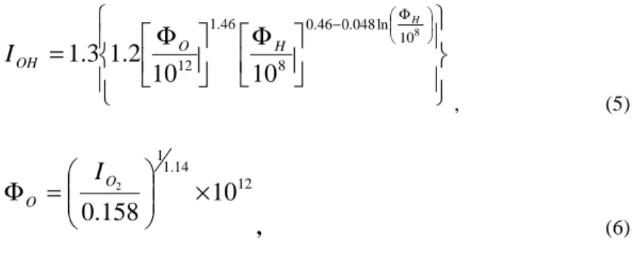
191 Φ Φ = Φ − 8 10 ln 048 . 0 46 . 0 8 46 . 1 12 10 10 2 . 1 3 . 1 H H O OH I , (5) 192 193 12 14 . 1 1 10 158 . 0 2 × = Φ O O I , (6) 194 195
where IOH is the nadir brightness of the OH(∆v=1) emission in kR, IO2 is the nadir brightness
196
of the O2(a1∆) emission in MR, ΦO and ΦH are the oxygen and the hydrogen vertical fluxes at
197
130 km expressed in cm-2 s-1, respectively. The nadir observations of the OH and the O2 198
intensities made by Krasnopolsky [2010] at 2130 LT between 35°N and 35°S have been 199
converted into limb intensities in order to be represented in Figure 4 by a square. He deduced 200
from a comparison with the model outputs that a hydrogen flux in equation (5) equal to 108 201
cm-2 s-1 best fits this observation. The model relation between the O2(a1∆) and the OH Meinel 202
brightness derived from (5) and (6) for this H flux value is represented in dashed line in 203
Figure 4. This curve passes through Krasnopolsky’s observation but does not fit well the high 204
O2 brightness values which were not considered in his study. Curves for other values of the 205
hydrogen flux have been plotted for comparison. It appears that a hydrogen flux of 108 cm-2 s -206
1
seems appropriate to fit the lowest values of the O2(a1∆) emission while a smaller value of 207
3x107 cm-2 s-1 (in dashed-dotted line) seems to better fit the highest intensities. However, 208
some points, with low O2 values but OH intensities greater than 1.5 MR, are not fitted, 209
whatever the hydrogen flux. A detailed inspection of the corresponding spectra confirmed the 210
relatively high OH to O2 intensity ratio. These points only represent less than 0.7% of all the 211
observations. 212
215 216
IV. Conclusions 217
218
The entire data set of VIRTIS-M-IR limb observations of the OH nightglow obtained 219
during the Venus Express mission has been analyzed for this study. To correctly estimate the 220
brightness of the OH(∆v=1) Meinel emission, the contribution of the thermal emission has 221
been subtracted. This process resulted in increasing the number of profiles compared to earlier 222
preliminary studies and adding lower OH intensity values to the data set. Our study indicates 223
that, globally, the observed peak brightness of the OH Meinel emission at the limb is very 224
variable, ranging from less than 20 kR to about 2 MR. 225
Statistics indicate that the OH intensity tends to be brighter near the antisolar point than 226
near the poles, although the associated level of confidence is low when individual 227
measurements are considered. This relatively low level of the correlation stems from the 228
extreme variability in individual observations, which is neither apparent in the binned data nor 229
in the preliminary results by Gérard et al. [2010] based on a limited sample. Our results 230
indicate that, as more OH observations are considered, the associated variability increases. By 231
contrast, although the OH peak altitude also appears to be variable, it shows no dependence 232
with the location on the nightside of Venus. 233
Some degree of correlation is expected between the brightness of the OH and the O2 234
emissions which have atomic oxygen as a common reactant in reactions (1) and (4) and as a 235
precursor to ozone involved in reaction (3). This relationship was numerically predicted by 236
the nightside model by Krasnopolsky [2010] for a given values of the downward fluxes of O 237
and H atoms. Our results suggest that the hydrogen flux is not constant. A hydrogen flux of 238
108 cm-2 s-1 best fits O2(a1∆) intensities from 0 to 40 MR, while a smaller value of 3x107 cm-2
s-1 better reproduces the higher brightness data (see Figure 4). As the highest O2(a1∆) intensity 240
values are statistically located near the antisolar point and decrease toward the poles [Piccioni 241
et al., 2009; Gérard et al., 2008], this could imply that the hydrogen flux is larger near the
242
pole than near the antisolar point. However, we note that, globally, the intensity level of the 243
OH nightglow is correctly predicted by the one-dimensional model of Venus’s nightside 244
photochemistry. Finally, it is important to keep in mind that horizontal transport plays an 245
important role in the redistribution of photochemically-produced species such as O, O3 and 246
minor long-lived species and possibly explains some of the variability of the OH emission and 247
its brightness relative to O2(a1∆). 248
249
Acknowledgments 250
251
We gratefully thank all members of the ESA Venus Express project and of the VIRTIS 252
scientific and technical teams. L. Soret was supported by the PRODEX program managed by 253
the European Space Agency with the help of the Belgian Federal Space Science Policy 254
Office. J.-C.G. acknowledges funding from the Belgian Fund for Scientific Research (FNRS). 255
This work was funded by Agenzia Spaziale Italiana and the Centre National d’Etudes 256
Spatiales. 257
References 258
259
Drossart, P., et al. (2007), Scientific goals for the observation of Venus by VIRTIS on 260
ESA/Venus Express mission, Planet. Space Sci., 55, 1653-1672, 261
doi:10.1016/j.pss.2007.01.003. 262
263
Gérard, J.-C., A. Saglam, G. Piccioni, P. Drossart, C. Cox, S. Erard, R. Hueso, and A. 264
Sánchez-Lavega (2008), Distribution of the O2 infrared nightglow observed with VIRTIS on 265
board Venus Express, Geophys. Res. Lett., 35, 2207, doi:10.1029/2007GL032021. 266
267
Gérard, J. C., C. Cox, L. Soret, A. Saglam, G. Piccioni, J._L. Bertaux, and P. Drossart (2009), 268
Concurrent observations of the ultraviolet nitric oxide and infrared O2 nightglow emissions 269
with Venus Express, J. Geophys. Res. Planets, 114, doi:E00b4410.1029/2009je003371. 270
271
Gérard, J.-C., L. Soret, A. Saglam, G. Piccioni, and P. Drossart (2010), The distributions of 272
the OH Meinel and O2(a1∆-X3Σ) nightglow emissions in the Venus mesosphere based on
273
VIRTIS observations, Adv. Space Res., doi:10.1016/j.asr.2010.01.022. 274
275
Krasnopolsky, V. A., Venus night airglow: ground-based detection of OH, Observations of O2 276
emissions, and photochemical model, Icarus, 2010, in press. 277
278
Meinel, A. B. (1950), OH emission bands in the spectrum of the night sky, Astrophys. J., 111, 279
565-564. 280
Piccioni, G., P. Drossart, L. Zasova, A. Migliorini, J.-C. Gérard, F. P. Mills, A. Shakun, A. 282
García Muñoz, N. Ignatiev, D. Grassi, V. Cottini, F. W. Taylor, S. Erard and the VIRTIS-283
Venus Express Technical Team (2008), First detection of hydroxyl in the atmosphere of 284
Venus, Astronomy and Astrophysics, 483-3, L29, doi:10.1051/0004-6361:200809761. 285
286
Piccioni, G., L. Zasova, A. Migliorini, P. Drossart, A. Shakun, A. García Muñoz, F. P. Mills, 287
A. Cardesín-Moinelo (2009), Near-IR oxygen nightglow observed by VIRTIS in the Venus 288
upper atmosphere, J. Geophys. Res., 114, E00B38, doi:10.1029/2008JE003133. 289
Figures 291
292
Figure 1: Limb profiles derived from orbits VI0499_11 (a) and 377_11 (b): raw data (thin 293
solid line), OH(∆v=1) emission (thick solid line) and Venus’s thermal emission (fit in dashed 294
line). 295
296
Figure 2: Distribution of the peak altitude (a) and brightness (b) along the line of sight of the 297
nightside OH(∆v=1) emission observed at the limb with VIRTIS-M-IR. As a comparison, 298
results previously obtained by Gérard et al. [2010] are represented with dashed lines. 299
300
Figure 3: Statistical distribution of the number of OH(∆v=1) infrared nightglow observations 301
grouped into 5° angular bins (a). The maximum limb brightness (b) and altitude (c) are plotted 302
as a function of the antisolar angle. The central values in each bin are the mean values and the 303
vertical bars indicate the asymmetric 1-σ variability in each bin. The solid line shows the 304
linear regression through the binned data points and the value of the linear correlation 305
coefficient R for the binned data is indicated. 306
307
Figure 4: Relationship between the maximum limb brightness of individual simultaneous OH 308
and O2(a1∆) limb profiles. The regression line through the data points is plotted in a black
309
solid line and the value of the correlation coefficient r is indicated. The square represents the 310
observation of Krasnopolsky [2010] at 2130 LT. The dashed line represents the calculated 311
relationship for a downward hydrogen flux of 108 atoms cm-2 s-1 at 130 km. 312
313 314 315
a
b
316 317 Figure 1 318 (a and b) 319 320a
b
321 322 Figure 2 323 (a and b) 324a
b
328 329 330 331 332 333 334 335 336 Figure 4 337 338 339 340 341 342