O
pen
A
rchive
T
OULOUSE
A
rchive
O
uverte (
OATAO
)
OATAO is an open access repository that collects the work of Toulouse researchers and
makes it freely available over the web where possible.
This is an author-deposited version published in :
http://oatao.univ-toulouse.fr/
Eprints ID : 12485
To link to this article : DOI :10.1109/ICNSC.2013.6548753
URL :
http://dx.doi.org/10.1109/ICNSC.2013.6548753
To cite this version : Guillaume, Romain and Thierry, Caroline and
Zielinski, Pawel
Robust Production Plan with Periodic Order Quantity
under Uncertain Cumulative Demands
. (2013) In: IEEE International
Conference on Networking, Sensing and Control - ICNSC, 10 April
2013 - 12 April 2013 (Paris, France).
Any correspondance concerning this service should be sent to the repository
administrator:
[email protected]
Robust Production Plan with Periodic Order
Quantity under Uncertain Cumulative Demands
Romain Guillaume Universit´e de Toulouse-IRIT
5, All´ees A. Machado 31058 Toulouse Cedex 1, France Email: [email protected]
Caroline Thierry Universit´e de Toulouse-IRIT
5, All´ees A. Machado 31058 Toulouse Cedex, France Email: [email protected]
Paweł Zieli´nski Institute of Mathematics
and Computer Science Wrocław University of Technology
Wybrze˙ze Wyspia´nskiego 27 50-370 Wrocław, Poland Email: [email protected]
Abstract—In this paper, we are interested in a production
planning process in collaborative supply chains. More precisely, we consider supply chains, where actors use Manufacturing Resource Planning process (MRPII). Moreover, these actors collaborate by sharing procurement plans. We focus on a supplier, who applies the Periodic Order Quantity (POQ) rule to plan a production integrating the uncertain procurement plan sent by her/his customer. The uncertainty of the procurement plan is expressed by closed intervals on the cumulative demands. In order to choose a robust production plan, under the interval uncertainty representation, the min-max criterion is applied.
We propose algorithms for determining the set of possible costs of a given production plan - due to the uncertainty on the cumulative demands. We then construct algorithms for computing a robust production plan with respect to the min-max criterion: the algorithm based on iterative adding constraints and the polynomial algorithms under certain realistic assumptions.
Index Terms—Supply Chain, Production Planning,
Uncer-tainty, Scenario Optimization.
I. INTRODUCTION
Companies today evolve in high competitive context that obliges the companies to collaborate with their suppliers and customers and creates uncertainty on the demand. Due to the well-known bullwhip effect [1], this uncertainty induces supply chain risks as backordering, obsolete inventory. Sharing information on the demand and the collaboration with the suppliers are ways to reduce this risk.
Most companies use Manufacturing Resource Planning (MRPII) to plan and control all resources of a manufacturing company. MRPII is composed of three processes (the pro-duction process, the procurement process and the distribution process) and three levels [2]: the strategic level (Sales and Operation Plan-S&OP), the tactical level (Master Production Scheduling (MPS) and Material Requirement Planning (MRP)) and the operational level (detailed scheduling and shop floor control). Within MRP process, different lot sizing rules exist for purchased or produced items, as Fixed Order Quantity (FOQ), Lot-for-Lot (L4L), Minimal Order Quantity (MOQ), Periodic Order Quantity (POQ), etc. In collaborative supply chains, collaboration is usually characterized by a set of point-to-point (customer/supplier) relationships with partial infor-mation sharing. More precisely, the collaboration process in supply chains, where actors use MRPII, is realized by sharing
procurement plans through the supply chain. The procurement plan can take into account uncertainty [3]. Thus, the problem is how to integrate this information in a production planning process. In this paper, we focus on cases where no probability distribution is available to model the uncertainty. In this context, the uncertainty is modeled by specifying a set of all possible realizations of the demand, called scenarios.
In the literature, the planning processes of MRPII have been extended to take into account the imprecision on quantities of period demands (MPS and MRP) [4], [5], [6], [7], quantities of period demands and uncertain orders (MRP) [8] and the imprecision on order quantities and dates with uncertain order (MRP) [9].
To deal with the uncertainty in the production planning, three approaches can be distinguished: computing the possible inventory and backordering levels over all scenarios to help the decision maker to choose a production plan ([4], [8], [9]), computing an optimal solution for one of possible demand scenarios [5], [6] and the robust optimization [10] under the scenario uncertainty representation, more precisely using the min-max criterion [7]. Under this criterion, we seek a solution that minimizes the largest cost over all scenarios. The cost function in production planning is the sum of inventory and backordering costs over the planning horizon.
The aim of this paper is to investigate the MRP process with the POQ rule under imprecision on cumulative demands. The POQ rule consists in producing a quantity equal to the gross requirements for 𝑃 periods minus any items in on-hand inventory plus any additional items needed to replenish safety stock if it has fallen below its desired level. To adapt the MRP with the POQ rule to the uncertain context, we have to consider the problem with backordering. Indeed, the problem without backordering is not satisfactory due to the fact that a solution method (without backordering) consists in applying the rule to the maximal cumulative demands. Thus, this solution method induces too much inventory and does not consider preferences of the decision maker between possible inventory and backordering levels. In the model proposed in this paper, the imprecision on the demand is represented by cumulative demand intervals. Such modeling allows us to describe the imprecision on order quantities and dates.
The paper is organized as follows. Section II presents the problem under consideration with the precise demands (pa-rameters). In Section III, we formulate the problem under the scenario uncertainty model in the robust optimization setting. We adopt min-max criterion to choose a robust production plan. We then propose algorithms for evaluating a given production plan (for determining optimal interval containing all possible values of costs of the production plan) and for computing an optimal robust production plan.
II. THEDETERMINISTICPROBLEM
In this section, a deterministic version of the problem under consideration, i.e. the problem in which all parameters are precisely known in advance.
Given 𝑇 + 1 periods. For period 𝑡, 𝑡 = 0, . . . , 𝑇 , let 𝑑𝑡 be the demand in period 𝑡, 𝑑𝑡 ≥ 0, 𝑥𝑡 the production amount in period 𝑡. Furthermore, we are given a periodicity 𝑃 , 𝑃 ∈ ℕ, such that:𝑥𝑡≥ 0 if 𝑡 = 𝑘 ⋅ 𝑃 ; otherwise (if 𝑡 ∕= 𝑘 ⋅ 𝑃 ) 𝑥𝑡= 0 for 𝑘 = 0, . . . , 𝑁 and 𝑡 = 0, . . . 𝑇 , where 𝑁 = 𝑇 /𝑃 (we assume without loss of generality that 𝑇 is divisible by 𝑃 ). Now, the set feasible production amounts 𝕏⊆ ℝ𝑇+1≥0 can be defined as follows: 𝕏= {𝑥𝑥𝑥 = (𝑥0, . . . , 𝑥𝑇) : 𝑥𝑡≥ 0 for 𝑡 = 𝑘 ⋅ 𝑃, 𝑥𝑡= 0 for 𝑡 ∕= 𝑘 ⋅ 𝑃, 𝑘 = 0, . . . , 𝑁, 𝑡 = 0, . . . , 𝑇 }. Set D𝑡 = ∑𝑡 𝑖=0𝑑𝑖 and X𝑡 = ∑𝑡 𝑖=0𝑥𝑖, D𝑡 and X𝑡 stand for the cumulative demand up to period𝑡 and the production level up to period𝑡, respectively. Obviously, X𝑡−1≤ X𝑡 and D𝑡−1≤ D𝑡,𝑡 = 1, . . . , 𝑇 . The nonnegative costs of carrying one unit of inventory from period𝑡 to period 𝑡 + 1 are given, denoted by𝑐𝐼, and all the inventory costs are equal for every period. The nonnegative costs of backordering one unit from period𝑡 + 1 to period 𝑡 are given, denoted by 𝑐𝐵, and all the backorder costs are equal for every period. Furthermore, we assume that𝑐𝐼 ≤ 𝑐𝐵. The nonnegative real function 𝐶
𝑡(𝑢, 𝑣) represents either the cost of storing inventory from period 𝑡 to period 𝑡 + 1 or the cost of backordering quantity from period𝑡 + 1 to period 𝑡, namely 𝐶𝑡(X𝑡, D𝑡) = 𝑐𝐼(X𝑡− D𝑡) if X𝑡≥ D𝑡;𝑐𝐵(D𝑡− X𝑡) otherwise. The function has the form 𝐶𝑡(X𝑡, D𝑡) = max{𝑐𝐼(X𝑡− D𝑡), 𝑐𝐵(D𝑡− X𝑡)}.
The optimization problem with the precise parameters con-sists in finding a feasible production plan𝑥𝑥𝑥 = (𝑥0, . . . , 𝑥𝑇), 𝑥𝑥𝑥 ∈ 𝕏, that minimizes the total cost of storage and backo-rdering subject to the conditions of satisfying each demand, that is min 𝑥 𝑥𝑥∈𝕏𝐹 (𝑥𝑥𝑥) = min𝑥𝑥𝑥∈𝕏 𝑇 ∑ 𝑡=0 𝐶𝑡 ( 𝑡 ∑ 𝑖=0 𝑥𝑖, 𝑡 ∑ 𝑖=0 𝑑𝑖 ) = min 𝑥 𝑥𝑥∈𝕏 𝑇 ∑ 𝑡=0 𝐶𝑡(X𝑡, D𝑡). (1) It is easily seen that when 𝑃 = 1, the problem (1) is equivalent to the classical lot sizing with backordering with the Lot-For-Lot (L4L) rule (see, e.g., [11], [12], [13]). The
problem (1) can be formulated as the minimum cost flow problem (see, e.g., [14]):
min 𝑇 ∑ 𝑡=0 (𝑐𝐼𝐼 𝑡+ 𝑐𝐵𝐵𝑡) s.t. 𝐵𝑡− 𝐼𝑡= 𝑡 ∑ 𝑗=0 (𝑑𝑗− 𝑥𝑗), 𝑡 = 0, . . . , 𝑇, 𝑥𝑡= 0, 𝑡 ∕= 𝑘 ⋅ 𝑃, 𝑘 = 0, . . . , 𝑁, 𝑡 = 0, . . . , 𝑇, 𝑥𝑡, 𝐵𝑡, 𝐼𝑡≥ 0, 𝑡 = 0, . . . , 𝑇. (2) The problem (2) can solved in𝑂(𝑇 ). For each 𝑘 = 0, . . . , 𝑁 − 1, we determine periods:
ℎ𝑘= max{𝑡 : 𝑡 ∈ {𝑘 ⋅ 𝑃, . . . , (𝑘 + 1) ⋅ 𝑃 − 1}, 𝑐𝐼(𝑡 − 𝑘 ⋅ 𝑃 ) ≤ 𝑐𝐵((𝑘 + 1) ⋅ 𝑃 − 𝑡)}. An optimal production plan to (2) is computed by the following formula for𝑡 = 0, . . . , 𝑇 and 𝑘 = 0, . . . , 𝑁 :
𝑥𝑡= ⎧ ⎨ ⎩ 0 if𝑡 ∕= 𝑘 ⋅ 𝑃 , Dℎ𝑘 if𝑡 = 𝑘 ⋅ 𝑃 and 𝑘 = 0, Dℎ𝑘− Dℎ𝑘−1 if𝑡 = 𝑘 ⋅ 𝑃 and 0 < 𝑘 < 𝑁 , D𝑘⋅𝑃− Dℎ𝑘−1 if𝑡 = 𝑘 ⋅ 𝑃 and 𝑘 = 𝑁 .
We have assumed that an initial inventory 𝐼 and an initial backorder 𝐵 are equal to zero. Otherwise, one can easily modify the above method to cope with𝐼 > 0 or 𝐵 > 0.
III. ROBUSTVERSION OF THEPROBLEM
In Section II, we have assumed the all input parameters in problem (1) are precisely known. However, in real life this is rarely the case. Here, we admit uncertainty on the demands.
A. Model of uncertainty
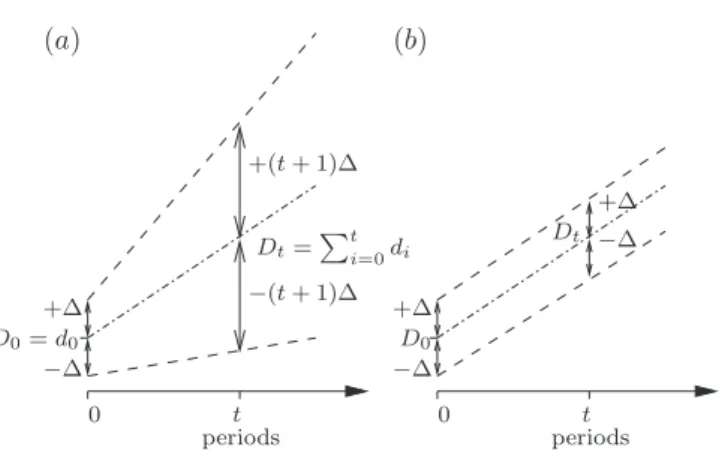
One of the simplest form of the uncertainty representations is modeling the imprecise demands ˜𝑑𝑡,𝑡 = 0, . . . , 𝑇 , as closed intervals[𝑑𝑡, 𝑑𝑡], 𝑑𝑡≥ 0, where 𝑑𝑡 and𝑑𝑡 are a minimal and a maximal possible values of demand ˜𝑑𝑡in period𝑡, respectively. So, assigning some interval[𝑑𝑡, 𝑑𝑡] to demand ˜𝑑𝑡means that it will take some value within the interval, but it is not possible to predict at present which one, i.e. 𝑑𝑡 ∈ [𝑑𝑡, 𝑑𝑡]. From the above model of uncertainty, it follows that the imprecision of cumulative demand D𝑡 = ∑𝑡 𝑖=0𝑑𝑖 increases in subsequent periods, i.e. D𝑡 ∈ [ ∑𝑡 𝑖=0𝑑𝑡, ∑𝑡 𝑖=0𝑑𝑡]. In fact, practitioners often express the knowledge on demand uncertainty by the range. The demand can be interpreted in two different ways: a demand in the period or a cumulative demand. For instance, a practitioner expresses the uncertainty on the demand by range ±Δ. If this uncertainty is interpreted as the one on demands in periods, then it leads to the cumulative demands with increasing uncertainty (see Fig. 1a)). This case is unrealistic compared to the case when the uncertainty is interpreted as the one on cumulative demands (see Fig. 1b)). So in this paper, the uncertainty of the demands ˜𝑑𝑡 is described by the uncertainty on the cumulative demands, modeled by intervals [D𝑡; D𝑡], instead of the uncertainty on demands in periods,
(𝑎) (𝑏) 𝑡 𝑡 0 0 +Δ +Δ +Δ 𝐷0= 𝑑0 𝐷0 𝐷𝑡 −Δ −Δ −Δ +(𝑡 + 1)Δ −(𝑡+ 1)Δ 𝐷𝑡= ∑𝑡 𝑖=0𝑑𝑖 periods periods
Fig. 1. An example: (a) the case with the uncertainty on demands in periods and the resulting uncertain cumulative demands, (b) the case with the uncertainty on cumulative demands.
modeled by [𝑑𝑡, 𝑑𝑡]. Hence, we are given intervals [D𝑡; D𝑡] that model the uncertainty of the cumulative demands for each period 𝑡, 𝑡 = 0, . . . , 𝑇 , where D𝑡 and D𝑡 are a minimal and a maximal possible values of cumulative demands in period𝑡, respectively. Obviously, D𝑡−1≤ D𝑡and D𝑡−1≤ D𝑡, 𝑡 = 1, . . . , 𝑇 .
A vector 𝑆 = (D0, . . . , D𝑇), D𝑡 ∈ [D𝑡; D𝑡], D𝑡−1 ≤ D𝑡, that represents an assignment of cumulative demands D𝑡 to periods 𝑡, 𝑡 = 0, . . . , 𝑇 , is called a scenario. Thus every scenario expresses a realization of the cumulative demands. It is easy to check that scenario𝑆 = (D0, . . . , D𝑇) induces an assignment of demands in periods 𝑡, 𝑡 = 0, . . . , 𝑇 . Namely, 𝑑𝑡 = D𝑡− D𝑡−1. We denote byΓ the set of all the scenarios, i.e.
Γ = {𝑆 = (D0, . . . , D𝑇) : D𝑡∈ [D𝑡; D𝑡], 𝑡 = 0, . . . , 𝑇, D𝑡−1≤ D𝑡, 𝑡 = 1, . . . , 𝑇 }. Among the scenarios ofΓ, we distinguish the ones called
ex-treme scenarios. Each extreme scenario𝑆 = (D𝑡)𝑇𝑡=0 belongs to the set of scenarios defined by the following recurrence formula: D𝑡∈ { {D0, D0} if𝑡 = 0, {max{D𝑡−1, D𝑡}, D𝑡} if 𝑡 = 1, . . . , 𝑇 . (3) We will denoted byΓext, the set of extreme scenarios. Clearly, Γext⊆ Γ. The cumulative demand and the demand in period 𝑡 under scenario 𝑆 are denoted by D𝑡(𝑆), D𝑡(𝑆) ∈ [D𝑡; D𝑡], and𝑑𝑡(𝑆), respectively, 𝑑𝑡(𝑆) = D𝑡(𝑆) − D𝑡−1(𝑆). Clearly, for every𝑆 ∈ Γ it holds D𝑡−1(𝑆) ≤ D𝑡(𝑆), 𝑡 = 1, . . . , 𝑇 . The function𝐶𝑡(X𝑡, D𝑡(𝑆)) = max{𝑐𝐼(X𝑡−D𝑡(𝑆)), 𝑐𝐵(D𝑡(𝑆)− X𝑡)}, represents either the cost of storing inventory from period 𝑡 to period 𝑡 + 1 or the cost of backordering quantity from period𝑡 + 1 to period 𝑡 under scenario 𝑆. Now 𝐹 (𝑥𝑥𝑥, 𝑆) denotes the total cost of a production plan 𝑥𝑥𝑥 ∈ 𝕏 under scenario 𝑆, i.e. 𝐹 (𝑥𝑥𝑥, 𝑆) = ∑𝑇
𝑡=0𝐶𝑡(X𝑡, D𝑡(𝑆)). The set feasible production amounts 𝕏 is the same as in Section II.
In order to choose a robust production plan, one of robust criteria, called the min-max can be adopted (see, e.g. [10]).
In the min-max version of problem (1), we seek a feasible production plan with the minimum the worst total cost over all scenarios, that is
ROB: min 𝑥𝑥𝑥∈𝕏𝐴(𝑥𝑥𝑥) = min𝑥𝑥𝑥∈𝕏max𝑆∈Γ𝐹 (𝑥𝑥𝑥, 𝑆) = min 𝑥 𝑥 𝑥∈𝕏max𝑆∈Γ 𝑇 ∑ 𝑡=0 𝐶𝑡(X𝑡, D𝑡(𝑆)). In other words, we wish to find among all production plans the one that minimizes the maximum production plan cost over all scenarios, that minimizes 𝐴(𝑥𝑥𝑥), 𝐴(𝑥𝑥𝑥) is the maximal cost of
production plan𝑥𝑥𝑥. An optimal solution 𝑥𝑥𝑥𝑟to the problem ROB is called optimal robust production plan.
Here and subsequently (as in Section II), we assume that an initial inventory𝐼 and an initial backorder 𝐵 are equal to zero. Otherwise, one can modify the algorithms presented in this section to cope with the case𝐼 > 0 or 𝐵 > 0.
B. Evaluating a Given Production Plan
In this section, we will be concerned with evaluating a given production plan. We will propose methods for computing the optimal interval containing all possible values of costs of the production plan.
Let 𝑥𝑥𝑥∗ ∈ 𝕏 be a given production plan. A scenario 𝑆𝑜 ∈ Γ that minimizes the total cost 𝐹 (𝑥𝑥𝑥∗, 𝑆) of the production plan𝑥𝑥𝑥∗ is called optimistic scenario. A scenario𝑆𝑤∈ Γ that maximizes the total cost 𝐹 (𝑥𝑥𝑥∗, 𝑆) of the production plan 𝑥𝑥𝑥∗ is called the worst case scenario. Thus, the optimal interval containing all possible values of costs of the production plan𝑥𝑥𝑥∗ is of form:[𝐹 (𝑥𝑥𝑥∗, 𝑆𝑜), 𝐹 (𝑥𝑥𝑥∗, 𝑆𝑤)]. We begin with a result on function𝐹 (𝑥𝑥𝑥∗, 𝑆) =∑𝑇
𝑡=0𝐶𝑡(X𝑡, D𝑡(𝑆)):
Proposition 1: Function𝐹 (𝑥𝑥𝑥∗, 𝑆) is convex on Γ for any fixed production plan𝑥𝑥𝑥∗∈ 𝕏.
Proposition 1 follows by similar arguments as in [7], i.e. function 𝑐𝐼
(X∗
𝑡 − D𝑡(𝑆)) and 𝑐𝐵(D𝑡(𝑆) − X∗𝑡) are convex on Γ and so max{𝑐𝐼(X∗ 𝑡 − D𝑡(𝑆)), 𝑐𝐵(D𝑡(𝑆) − X∗𝑡)} and ∑𝑇 𝑡=0max{𝑐 𝐼 (X∗ 𝑡 − D𝑡(𝑆)), 𝑐𝐵(D𝑡(𝑆) − X∗𝑡)} are convex.
1) Computing an Optimistic Scenario: The problem of determining an optimistic scenario𝑆𝑜
= (D𝑜
𝑡)𝑇𝑡=0for a given production plan𝑥𝑥𝑥∗∈ 𝕏, i.e. the problem
𝐹 (𝑥𝑥𝑥∗, 𝑆𝑜) = min 𝑆∈Γ𝐹 (𝑥𝑥𝑥
∗, 𝑆), (4)
can be formulated by a linear programming problem: min 𝑇 ∑ 𝑡=0 (𝑐𝐼𝐼 𝑡+ 𝑐𝐵𝐵𝑡) s.t. 𝐵𝑡− 𝐼𝑡= D𝑡− X∗𝑡, 𝑡 = 0, . . . , 𝑇, D𝑡−1≤ D𝑡, 𝑡 = 1, . . . , 𝑇, D𝑡≤ D𝑡≤ D𝑡, 𝑡 = 0, . . . , 𝑇. 𝐵𝑡, 𝐼𝑡≥ 0, 𝑡 = 0, . . . , 𝑇 (5) If D𝑜
𝑡, 𝐵𝑡𝑜 and 𝐼𝑡𝑜 is an optimal solution to (5), then 𝑆𝑜 = (D𝑜
𝑡)𝑇𝑡=0 is an optimistic scenario for𝑥𝑥𝑥∗. Furthermore, since 𝑐𝐼, 𝑐𝑏≥ 0, either 𝐼𝑜
𝑡 > 0 or 𝐵𝑡𝑜> 0, which means that for 𝑆𝑜 storing from period𝑡 to 𝑡+1 and backordering from period 𝑡+1 to 𝑡 are not performed simultaneously. However, determining
an optimistic scenario for𝑥𝑥𝑥∗can be improved to𝑂(𝑇 ), since one can give the explicit form of an optimistic scenario𝑆𝑜= (D𝑜
𝑡)𝑇𝑡=0and thus an optimal solution to (5):
D𝑜𝑡 = ⎧ ⎨ ⎩ D𝑡 if X∗𝑡 < D𝑡, X∗𝑡 if D𝑡≤ X∗𝑡 ≤ D𝑡,𝑡 = 0, . . . , 𝑇 . D𝑡 if X∗𝑡 > D𝑡, (6)
The form (6) follows from inequalities: D𝑡−1≤ D𝑡, D𝑡−1≤ D𝑡, X∗𝑡−1≤ X∗𝑡,𝑡 = 1, . . . , 𝑇 , and Proposition 1.
2) Computing a Worst Case Scenario: We now pass on to the problem of computing a worst case scenario 𝑆𝑤 = (D𝑤
𝑡 )𝑇𝑡=0for a given production plan𝑥𝑥𝑥∗∈ 𝕏, i.e. 𝐹 (𝑥𝑥𝑥∗, 𝑆𝑤) = max
𝑆∈Γ𝐹 (𝑥𝑥𝑥
∗, 𝑆). (7)
Problem (7) is more difficult than the one of computing an optimistic scenario and thus a solution algorithm is much more involved. The following proposition allows us to construct an efficient algorithm for the problem under consideration:
Proposition 2: A worst case scenario𝑆𝑤is an extreme one, i.e.𝑆𝑤 ∈ Γ
ext.
Proof: Proposition follows by the same method as [7]. Function𝐹 (𝑥𝑥𝑥∗, 𝑆) attains its maximum in convex set Γ. An easy computation shows that scenarios 𝑆 ∈ Γext are the vertices of Γ. From the above and Proposition 1, it follows that𝐹 (𝑥𝑥𝑥∗, 𝑆) attains the maximum value at a vertex of Γ (see, e.g., [15]).
We now construct an algorithm for the problem (7), based on a dynamic programming technique. Let 𝔻𝑡 be the set of feasible cumulative demand levels in period 𝑡, 𝑡 = 0, . . . , 𝑇 . Namely D𝑡 ∈ 𝔻𝑡 if and only if D𝑡 is the 𝑡th component of an extreme scenario that belongs to the set generated by formula (3) (Γext). Let C𝑡−1(D𝑡−1) be the maximal cost of a given production plan 𝑥𝑥𝑥∗ over periods 𝑡, . . . , 𝑇 , when the cumulative demand level up to period𝑡 − 1 is equal to D𝑡−1, D𝑡−1∈ 𝔻𝑡−1, C𝑡−1: 𝔻𝑡−1→ ℝ≥0. Set 𝔻−1= {0}. We see at once that: C𝑇(D𝑇) = 0, D𝑇 ∈ 𝔻𝑇, (8) C𝑡−1(D𝑡−1) = max ⎧ ⎨ ⎩ 𝐶𝑡(X∗𝑡, D𝑡) + C𝑡(D𝑡) 𝐶𝑡(X∗𝑡, max{D𝑡−1, D𝑡})+ +C𝑡(max{D𝑡−1, D𝑡}) ⎫ ⎬ ⎭ D𝑡−1∈ 𝔻𝑡−1, 𝑡 = 𝑇, . . . , 0. (9) The maximal cost of production plan𝑥𝑥𝑥∗over period0, . . . , 𝑇 is equal to C−1(0), C−1(0) = 𝐹 (𝑥𝑥𝑥∗, 𝑆𝑤), which is computed by the backward recursion (8) and (9). Worst case scenario𝑆𝑤= (D𝑤
𝑡 )𝑇𝑡=0 for 𝑥𝑥𝑥∗ can be determined by a forward recursion technique. It is sufficient to store for each D𝑡−1 ∈ 𝔻𝑡−1 the value for which the maximum in (9) is attained, that is D𝑤𝑡 is eithermax{D𝑡−1, D𝑡} or D𝑡.
Let us analyze the running time of the dynamic program-ming based algorithm. Building the sets of feasible cumula-tive demand levels 𝔻0, . . . , 𝔻𝑇 according to formula (3) and computing 𝐹 (𝑥𝑥𝑥∗, 𝑆𝑤) by the backward recursion (8) and (9) can be done in𝑂(𝑇 ⋅ max𝑡=0,...,𝑇∣𝔻𝑡∣). Determining 𝑆𝑤 by
by a forward recursion takes 𝑂(𝑇 ). It is easy to check that max𝑡=0,...,𝑇∣𝔻𝑡∣ ≤ 𝑇 + 2. Hence, the total running time of the algorithm is𝑂(𝑇2).
C. Computing an Optimal Robust Production Plan
In this section, we will propose algorithms for computing an optimal robust production plan to problem ROB. We will first construct an algorithm for problem ROB without any additional restrictions on ROB. We will then put some restrictions on ROB and obtain more efficient algorithms for computing an optimal robust production plan.
1) Algorithm for the General Problem ROB: We now give an iterative algorithm for the problem ROB based on iterative adding constraints for min-max problems proposed in [16]. Similar methods were developed for min-max regret linear programming problems with an interval objective func-tion [17], [18] and a producfunc-tion planning problem with interval demands [7]. Let us perform a relaxation of the problem ROB that consists in replacing a given cumulative demand scenario set Γ with a discrete scenario set Γdis = {𝑆1, . . . , 𝑆𝐾}, Γdis⊆ Γ: RX-ROB: 𝑧 = min 𝑧ˆ s.t. 𝑧 ≥ 𝐹 (𝑥𝑥𝑥, 𝑆𝑖) ∀𝑆𝑖∈ Γ dis, 𝑥𝑥𝑥 ∈ 𝕏, (10) where𝑆𝑖= (D𝑖
𝑡)𝑇𝑡=0,𝑥𝑥𝑥 = (𝑥𝑡)𝑇𝑡=0. SinceΓdis⊆ Γ, ˆ𝑧 is a lower bound on the maximal cost of an optimal robust production plan𝑥𝑥𝑥𝑟 to problem ROB,𝑧 ≤ 𝐴(𝑥ˆ 𝑥𝑥𝑟) = 𝐹 (𝑥𝑥𝑥𝑟, 𝑆𝑤). Note that the constraint 𝑣 ≥ 𝐹 (𝑥𝑥𝑥, 𝑆𝑖) called scenario cut, associated with𝑆𝑖is not a linear constraint. Each scenario cut associated with 𝑆𝑖 can be linearized by replacing it with the following 𝑇 +2 constraints and 2𝑇 +2 new decision variables (𝐵𝑖
𝑡and𝐼𝑡𝑖): 𝑧 ≥ 𝑇 ∑ 𝑡=0 (𝑐𝐼𝐼𝑖 𝑡 + 𝑐 𝐵𝐵𝑖 𝑡), 𝐵𝑖 𝑡− 𝐼𝑡𝑖= D 𝑖 𝑡− 𝑡 ∑ 𝑗=0 𝑥𝑗, 𝑡 = 0, . . . , 𝑇, 𝐵𝑖 𝑡, 𝐼𝑡𝑖≥ 0, 𝑡 = 0, . . . , 𝑇. (11)
Replacing each scenario cut 𝑧 ≥ 𝐹 (𝑥𝑥𝑥, 𝑆𝑖) by (11) in (10) leads to the following linear program:
ˆ 𝑧 = min 𝑧 s.t. 𝑧 ≥ 𝑇 ∑ 𝑡=0 (𝑐𝐼𝐼𝑖 𝑡+ 𝑐𝐵𝐵𝑡𝑖), ∀𝑆𝑖∈ Γdis, 𝐵𝑖 𝑡− 𝐼𝑡𝑖= D 𝑖 𝑡− 𝑡 ∑ 𝑗=0 𝑥𝑗, 𝑡 = 0, . . . , 𝑇 , ∀𝑆𝑖∈ Γdis, 𝐵𝑖 𝑡, 𝐼𝑡𝑖≥ 0, 𝑡 = 0, . . . , 𝑇 , ∀𝑆𝑖∈ Γdis, 𝑥𝑡= 0, 𝑡 ∕= 𝑘 ⋅ 𝑃 , 𝑘 = 0, . . . , 𝑁, 𝑡 = 0, . . . , 𝑇, 𝑥𝑡≥ 0, 𝑡 = 0, . . . , 𝑇. (12) The iterative algorithm for the problem ROB (Algorithm 1) starts with zero lower bound 𝐿𝐵 = 0, a candidate ˆ𝑥𝑥𝑥 ∈ 𝕏 for an optimal solution for ROB (any solution in 𝕏) and
empty discrete scenario set, Γdis = ∅. At each iteration, a worst case scenario 𝑆𝑤 for 𝑥𝑥𝑥 is determined by the dy-ˆ namic programming algorithm presented in Section III-B2. The value of𝐴(ˆ𝑥𝑥𝑥) = 𝐹 (ˆ𝑥𝑥𝑥, 𝑆𝑤) is an upper bound on 𝐴(𝑥𝑥𝑥𝑟), 𝐴(𝑥𝑥𝑥𝑟) ≤ 𝐴(ˆ𝑥𝑥𝑥). If a termination criterion is fulfilled (Step 3), for a given precision 𝜖 > 0, then the algorithm stops with production plan𝑥𝑥ˆ𝑥 being an approximation of an optimal robust production plan𝑥𝑥𝑥𝑟. Otherwise the worst case scenario𝑆𝑤 is added toΓdis, the scenario cut corresponding to𝑆𝑤is appended to problem RX-ROB or equivalently to linear programming problem (12) . Next the updated linear programming prob-lem (12) is solved to obtain a better candidate𝑥𝑥𝑥 for an optimalˆ robust production plan 𝑥𝑥𝑥𝑟 to problem ROB and new lower bound𝐿𝐵 = ˆ𝑧. Since set Γdisis updated during the course of the algorithm, the computed values of lower bounds{ˆ𝑧} form a nondecreasing sequence of their values. Then new iteration is started.
Algorithm 1: Solving problem ROB.
Input:[D𝑡, D𝑡, ], 𝑡 = 0, . . . 𝑇 , 𝑐 𝐼
,𝑐𝐵
, initial production plan𝑥ˆ𝑥𝑥 ∈ 𝕏, a tolerance 𝜖 > 0.
Output: A production plan, an approximation of an optimal
robust production plan, and its worst case scenario.
Step 0.𝑖 := 0, 𝐿𝐵 := 0, Γdis:= ∅.
Step 1.𝑥𝑥𝑥𝑖
:= ˆ𝑥𝑥𝑥.
Step 2. Compute a worst case scenario𝑆𝑤
for𝑥𝑥𝑥𝑖
by the dynamic programming algorithm presented in Section III-B2.
Step 3.Δ := 𝐹 (𝑥𝑥𝑥𝑖 , 𝑆𝑤 ) − 𝐿𝐵. If 𝐿𝐵 > 1 then Δ := Δ/𝐿𝐵. IfΔ ≤ 𝜖 then output 𝑥𝑥𝑥𝑖 , 𝑆𝑤 and STOP. Step 4.𝑖 := 𝑖 + 1, 𝑆𝑖 := 𝑆𝑤 ,Γdis:= Γdis∪ {𝑆 𝑖 } and append scenario cut𝑧 ≥ 𝐹 (𝑥𝑥𝑥, 𝑆𝑖 ) to problem RX-ROB.
Step 5. Compute an optimal solution(ˆ𝑥𝑥𝑥, ˆ𝑧) to RX-ROB (linear programming problem (12)),𝐿𝐵 := ˆ𝑧, and go to Step 1.
Algorithm 1 terminates in a finite number of iterations for any given 𝜖 > 0. In order to show this, the same reasoning applies as those given in [19, Theorem 2.5], [16, Theorem 3] and [7, Theorem 3]. It is worth pointing out that the running time of each iteration highly depends on Step 2 and Step 5, where a worst case scenario is computed and linear program-ming problem (12) is solved. The running time of Step 2 is 𝑂(𝑇2), linear program (12) (Step 5) can be solved by using a specially-tuned method for this kind of problems [20] or by some standard off-the-shelf LP solvers. Hence, each iteration of Algorithm 1 can be done efficiently (in a polynomial time).
2) Algorithms for Special Cases of ROB: Consider the problem ROB, when periodicity 𝑃 = 1. In this case, we can apply a method proposed in [7] for computing an optimal robust production plan𝑥𝑥𝑥𝑟 = (𝑥𝑟
𝑡)𝑇𝑡=0: X𝑟𝑡 = 𝑐𝐵 D𝑡+ 𝑐𝐼D𝑡 𝑐𝐵+ 𝑐𝐼 , 𝑡 = 0, . . . , 𝑇. (13) Set𝑥𝑟 0= X𝑟0 and𝑥𝑟𝑡 = X𝑟𝑡− X𝑟𝑡−1 for𝑡 = 1, . . . , 𝑇 .
Consider the problem ROB, when𝑃 > 1 (if 𝑃 = 1 one can use (13)) and the bounds of cumulative demand intervals are such that D𝑡−1≤ D𝑡for every𝑡 = 1, . . . , 𝑇 . According to the above assumption, the set of cumulative demand scenarios Γ
has the form Γ = [D0, D0] × ⋅ ⋅ ⋅ × [D𝑇, D𝑇]. Now each 𝑆 = (D𝑡)𝑇𝑡=0 ∈ Γ has components such that D𝑡−1 ≤ D𝑡, 𝑡 = 1, . . . , 𝑇 . Hence, and the periodicity in the problem ROB, it follows that one can decompose the problem into 𝑁 + 1 separate subproblems, that is:
𝑥 𝑥 𝑥𝑟= arg min 𝑥𝑥𝑥∈𝕏max𝑆∈Γ 𝑇 ∑ 𝑡=0 𝐶𝑡(X𝑡, D𝑡(𝑆)) = = 𝑁−1 ∑ 𝑘=0 min X𝑘⋅𝑃∈𝒳𝑘 max 𝑆∈Γ𝑘 (𝑘+1)⋅𝑃 −1 ∑ 𝑡=𝑘⋅𝑃 𝐶𝑡(X𝑘⋅𝑃, D𝑡(𝑆)) + min X𝑁⋅𝑃∈𝒳𝑁 max 𝑆∈Γ𝑁𝐶𝑁⋅𝑃(X𝑁⋅𝑃, D𝑁⋅𝑃(𝑆)), (14) where𝒳𝑘 = [D𝑘⋅𝑃, D𝑘⋅𝑃] ∪ ⋅ ⋅ ⋅ ∪ [D(𝑘+1)⋅𝑃 −1, D(𝑘+1)⋅𝑃 −1], Γ𝑘 = [D𝑘⋅𝑃, D𝑘⋅𝑃] × ⋅ ⋅ ⋅ × [D(𝑘+1)⋅𝑃 −1, D(𝑘+1)⋅𝑃 −1], 𝑘 = 0, . . . , 𝑁 −1, 𝒳𝑁 = [D𝑁⋅𝑃, D𝑁⋅𝑃] and Γ𝑁 = [D𝑁⋅𝑃, D𝑁⋅𝑃]; Γ = Γ0× ⋅ ⋅ ⋅ × Γ𝑁. Obviously, the above possible cumulative production levels are nondecreasing sequence of their values, X0 ≤ X𝑃 ≤ ⋅ ⋅ ⋅ ≤ X𝑁⋅𝑃. Therefore, we need only to solve the𝑁 + 1 separate subproblems. The last subproblem is trivial, i.e. an optimal cumulative production level X𝑟
𝑁⋅𝑃 can be computed by formula: X𝑟𝑁⋅𝑃 = 𝑐𝐵 D𝑁⋅𝑃+ 𝑐𝐼D𝑁⋅𝑃 𝑐𝐵+ 𝑐𝐼 . (15)
It remains to solve the subproblems for𝑘 = 0, . . . , 𝑁 − 1, i.e. min X𝑘⋅𝑃∈𝒳𝑘 max 𝑆∈Γ𝑘 (𝑘+1)⋅𝑃 −1 ∑ 𝑡=𝑘⋅𝑃 𝐶𝑡(X𝑘⋅𝑃, D𝑡(𝑆)). (16) Consider the𝑘th subproblem. Since X𝑡 = X𝑘⋅𝑃 in period 𝑡, 𝑡 ∈ {𝑘 ⋅ 𝑃 + 1, . . . , (𝑘 + 1) ⋅ 𝑃 − 1}, worst case scenar-ios 𝑆𝑤 ∈ Γ𝑘 for X
𝑘⋅𝑃 belong to the set [D𝑘⋅𝑃, D𝑘⋅𝑃] × ⋅ ⋅ ⋅ × [Dℎ−1, Dℎ−1] × [Dℎ, Dℎ] × [Dℎ+1, Dℎ+1] × ⋅ ⋅ ⋅ × [D(𝑘+1)⋅𝑃 −1, D(𝑘+1)⋅𝑃 −1] ⊆ Γ𝑘, assuming that X𝑘⋅𝑃 ∈ [Dℎ, Dℎ].
For each ℎ = 𝑘 ⋅ 𝑃, . . . , (𝑘 + 1) ⋅ 𝑃 − 1, we compute a possible cumulative production level
Xℎ𝑘⋅𝑃 = 𝑐𝐵D
ℎ+ 𝑐𝐼Dℎ
𝑐𝐵+ 𝑐𝐼 ∈ [Dℎ, Dℎ]. Note that for Xℎ
𝑘⋅𝑃 equality𝐶ℎ(Xℎ𝑘⋅𝑃, Dℎ) = 𝐶ℎ(Xℎ𝑘⋅𝑃, Dℎ) holds and its worst case scenario has form (D𝑘⋅𝑃, . . . , Dℎ−1, Dℎ, . . . , D(𝑘+1)⋅𝑃 −1). Thus, the worst case cost for Xℎ𝑘⋅𝑃 over the set of scenarios Γ𝑘, denoted by 𝐶ℎ, is as follows: 𝐶ℎ (Xℎ 𝑘⋅𝑃) = max 𝑆∈Γ𝑘 (𝑘+1)⋅𝑃 −1 ∑ 𝑡=𝑘⋅𝑃 𝐶𝑡(Xℎ𝑘⋅𝑃, D𝑡(𝑆)) = ℎ−1 ∑ 𝑡=𝑘⋅𝑃 𝐶𝑡(Xℎ𝑘⋅𝑃, D𝑡) + (𝑘+1)⋅𝑃 −1 ∑ 𝑡=ℎ 𝐶𝑡(Xℎ𝑘⋅𝑃, D𝑡). We then determine an optimal cumulative production level X𝑟
𝑘⋅𝑃 for the𝑘th subproblem (16) by formula: X𝑟𝑘⋅𝑃 = arg min
ℎ∈{𝑘⋅𝑃,...,(𝑘+1)⋅𝑃 −1}𝐶 ℎ
Using (15) and (17), one can easily compute an optimal robust production plan𝑥𝑥𝑥𝑟. Thus, (14) can be solved in𝑂(𝑇 ).
IV. CONCLUSION
In this paper, we have studied the possibility of integrating the uncertainty into planning process. We have proposed effi-cient algorithms for solving the production planning problem using MRP process with the POQ rule under uncertain cu-mulative demands, modeled by closed intervals, with the min-max criterion. Namely, the algorithm based on iterative adding constraints. It is worth pointing out that each iteration can done in a polynomial time. Moreover, we have provided algorithms for two special cases of the problem under consideration. The first case corresponds to the Lot-For-Lot (L4L) rule. In the second one the range of uncertainty is small compared to the demand.
An interesting topic for further research is investigating the production planning problem using MRP process under uncertain cumulative demands, considered in this paper, with other rules such as: Fixed Order Quantity (FOQ) and Minimal Order Quantity (MOQ), and with production constraints.
REFERENCES
[1] H. L. Lee, V. Padmanabhan, and S. Whang, “Information Distortion in a Supply Chain: The Bullwhip Effect,” Management Science, vol. 43, pp. 546–558, 1997.
[2] J. R. T. Arnold, S. N. Chapman, and L. M. Clive, Introduction to
Materials Management, 7th ed. Prentice Hall, 2011.
[3] A. A. Zouggar, J. C. Deschamps, and J. P. Bourri`eres, “Supply Chain Reactivity Assessment Regarding Two Negotiated Commitments: Frozen Horizon and Flexibility Rate,” in Advances in Production Management
Systems. New Challenges, New Approaches, ser. IFIP Advances in Information and Communication Technology, B. Vallespir and T. Alix, Eds., vol. 338. Springer-Verlag, 2010, pp. 179–186.
[4] H. Fargier and C. Thierry, “The Use of Possibilistic Decision Theory in Manufacturing Planning and Control: Recent Results in Fuzzy Master Production Scheduling,” in Advances in Scheduling and Sequencing
under Fuzziness, R. Slowi´nski and M. Hapke, Eds. Springer-Verlag, 2000, pp. 45–59.
[5] J. Mula, R. Poler, and J. P. Garcia-Sabater, “Material Requirement Planning with fuzzy constraints and fuzzy coefficients,” Fuzzy Sets and
Systems, vol. 159, pp. 783–793, 2007.
[6] R. Tavakkoli-Moghaddam, M. Rabbani, A. H. Gharehgozli, and N. Za-erpour, “A Fuzzy Aggregate Production Planning Model for Make-to-Stock Environments,” in Proceedings of the International Conference on
Industrial Engineering and Engineering Management, 2007, pp. 1609– 1613.
[7] R. Guillaume, P. Kobyla´nski, and P. Zieli´nski, “A robust lot sizing problem with ill-known demands,” Fuzzy Sets and Systems, vol. 206, pp. 39–57, 2012.
[8] B. Grabot, L. Geneste, G. Reynoso-Castillo, and S. V´erot, “Integration of uncertain and imprecise orders in the MRP method,” Journal of
Intelligent Manufacturing, vol. 16, pp. 215–234, 2005.
[9] R. Guillaume, C. Thierry, and B. Grabot, “Modelling of ill-known re-quirements and integration in production planning,” Production Planning
and Control, vol. 22, pp. 336–352, 2011.
[10] P. Kouvelis and G. Yu, Robust Discrete Optimization and its applications. Kluwer Academic Publishers, 1997.
[11] L. A. Johnson and D. C. Montgomery, Operations Research in
Produc-tion Planning, Scheduling and Inventory Control. John Wiley & Sons, 1974.
[12] H. M. Wagner and T. M. Whitin, “Dynamic Version of the Economic Lot Size Model,” Management Science, vol. 5, pp. 89–96, 1958. [13] M. Florian, K. J. Lenstra, and A. H. G. Rinnooy Kan, “Deterministic
Pro-duction Planning: Algorithms and Complexity,” Management Science, vol. 26, pp. 669–679, 1980.
[14] R. K. Ahuja, T. L. Magnanti, and J. B. Orlin, Network Flows: theory,
algorithms, and applications. Englewood Cliffs, New Jersey: Prentice Hall, 1993.
[15] B. Martos, Nonlinear programming theory and methods. Budapest: Akad´emiai Kiad´o, 1975.
[16] K. Shimizu and E. Aiyoshi, “Necessary Conditions for Min-Max Prob-lems and Algorithms by a Relaxation Procedure,” IEEE Transactions on
Automatic Control, vol. 25, pp. 62–66, 1980.
[17] M. Inuiguchi and M. Sakawa, “Minimax regret solution to linear programming problems with an interval objective function,” European
Journal of Operational Research, vol. 86, pp. 526–536, 1995. [18] H. E. Mausser and M. Laguna, “A heuristic to minimax absolute
regret for linear programs with interval objective function coefficients,”
European Journal of Operational Research, vol. 117, pp. 157–174, 1999. [19] A. M. Geoffrion, “Generalized Benders Decomposition,” Journal of
Optimization Theory and Applications, vol. 10, pp. 237–260, 1972. [20] R. K. Ahuja, “Minimax linear programming problem,” Operations