Pépite | Apprentissage séquentiel efficace dans des environnements structurés avec contraintes

Texte intégral

(1)Thèse de Daniele Calandriello, Lille 1, 2017. Efficient Sequential Learning in Structured and Constrained Environments Daniele Calandriello. © 2017 Tous droits réservés.. lilliad.univ-lille.fr.

(2) Thèse de Daniele Calandriello, Lille 1, 2017. THÈSE DE DOCTORAT UNIVERSITÉ LILLE 1. Centre de Recherche en Informatique, Signal et Automatique de Lille. Thése de doctorat. Spécialité : Informatiques. présentée par. Daniele Calandriello. Efficient Sequential Learning in Structured and Constrained Environments sous la direction de M. Michal VALKO et le co-encadrement de M. Alessandro LAZARIC. Rapporteurs :. M. M.. Nicolò Michael. CESA-BIANCHI MAHONEY. Università di Milano UC Berkeley. Soutenue publiquement le 18 Decembre 2017 devant le jury composé de. M. M. M. Mme. M. M.. © 2017 Tous droits réservés.. Nicolò Michael Francis Mylène Michal Alessandro. CESA-BIANCHI MAHONEY BACH MAÏDA VALKO LAZARIC. Università di Milano UC Berkeley INRIA-ENS Université Lille 1 INRIA INRIA. Rapporteur Rapporteur Examinateur Examinateur Directeur Co-Directeur. lilliad.univ-lille.fr.

(3) Thèse de Daniele Calandriello, Lille 1, 2017. To whom it shall matter. © 2017 Tous droits réservés.. lilliad.univ-lille.fr.

(4) Thèse de Daniele Calandriello, Lille 1, 2017. 4. Abstract The main advantage of non-parametric models is that the accuracy of the model (degrees of freedom) adapts to the number of samples. The main drawback is the so-called "curse of kernelization": to learn the model we must first compute a similarity matrix among all samples, which requires quadratic space and time and is unfeasible for large datasets. Nonetheless the underlying effective dimension (effective d.o.f.) of the dataset is often much smaller than its size, and we can replace the dataset with a subset (dictionary) of highly informative samples. Unfortunately, fast data-oblivious selection methods (e.g., uniform sampling) almost always discard useful information, while data-adaptive methods that provably construct an accurate dictionary, such as ridge leverage score (RLS) sampling, have a quadratic time/space cost. In this thesis we introduce a new single-pass streaming RLS sampling approach that sequentially construct the dictionary, where each step compares a new sample only with the current intermediate dictionary and not all past samples. We prove that the size of all intermediate dictionaries scales only with the effective dimension of the dataset, and therefore guarantee a per-step time and space complexity independent from the number of samples. This reduces the overall time required to construct provably accurate dictionaries from quadratic to near-linear, or even logarithmic when parallelized. Finally, for many non-parametric learning problems (e.g., K-PCA, graph SSL, online kernel learning) we we show that we can can use the generated dictionaries to compute approximate solutions in near-linear that are both provably accurate and empirically competitive.. Résumé L’avantage principal des méthodes d’apprentissage non-paramétriques réside dans le fait que la nombre de degrés de libertés du modèle appris s’adapte automatiquement au nombre d’échantillons. Ces méthodes sont cependant limitées par le "fléau de la kernelisation": apprendre le modèle requière dans un premier temps de construire une matrice de similitude entre tous les échantillons. La complexité est alors quadratique en temps et espace, ce qui s’avère rapidement trop coûteux pour les jeux de données de grande dimension. Cependant, la dimension "effective" d’un jeu de donnée est bien souvent beaucoup plus petite que le nombre d’échantillons lui-même. Il est alors possible de substituer le jeu de donnée réel par un jeu de données de taille réduite (appelé "dictionnaire") composé exclusivement d’échantillons informatifs. Malheureusement, les méthodes avec garanties théoriques utilisant des dictionnaires comme "Ridge Leverage Score" (RLS) ont aussi une complexité quadratique. Dans cette thèse nous présentons une nouvelle méthode d’échantillonage RLS qui met à jour le dictionnaire séquentiellement en ne comparant chaque nouvel échantillon qu’avec le dictionnaire actuel, et non avec l’ensemble des échantillons passés. Nous montrons que la taille de tous les dictionnaires ainsi construits est de l’ordre de la dimension effective du jeu de données final, guarantissant ainsi une complexité en temps et espace à chaque étape indépendante du nombre total d’échantillons. Cette méthode présente l’avantage de pouvoir être parallélisée. Enfin, nous montrons que de nombreux problèmes d’apprentissage non-paramétriques peuvent être résolus de manière approchée grâce à notre méthode.. © 2017 Tous droits réservés.. lilliad.univ-lille.fr.

(5) Thèse de Daniele Calandriello, Lille 1, 2017. © 2017 Tous droits réservés.. lilliad.univ-lille.fr.

(6) Thèse de Daniele Calandriello, Lille 1, 2017. Acknowledgements My gratitude goes to my advisors, Alessandro Lazaric and Michal Valko. Thanking them for teaching me how to be a good scientist would be telling only half of the story, as showing me how to be professional has been priceless for my growth. The hardest part of sequential learning is credit assignment, but it is not difficult for me to see that it is thanks to your advice that I can now face and solve many more problems, in academia and life. My thanks extend to the whole SequeL team. Thank you Frédéric, Tomá˘s, Julien, Jean-Bastien, Ronan, Matteo, Alexandre, Florian, and all the other PhDs. It is much more fun to march for a deadline when you have the right company. Thank you to Philippe, Olivier, Jérémie, Romaric, Emilie, Daniil, Odalric, and the other permanents. It has been an exciting experience to work in a group where every day you could discuss about something new with an expert on the topic. A special thank to Yiannis Koutis, whose work on graphs set me off on my research, and whose help gave me an extra push at critical moments of my PhD. I am also thankful to my reviewers, Michael Mahoney and Nicolò Cesa-Bianchi, for laying the foundations of the problems discussed in this thesis, and to the whole thesis committee. My PhD would not have been possible today without all the support I received in the past. Grazie Mom, Dad, Franci and Stefi for pushing me when I needed and keeping me grounded. This thesis might be finished, but I hope you will keep asking me how my algorithms are doing for many years to come. And grazie also to my friends Andrea, Matteo, Piero, Lillo, Lanci and Luca that balanced days spent between abstractions. Most of all, this thanks can not be finished without thanking my Ştefana, just as a day would not be finished without her bringing me inspiration and ungrumpification. Having you made me a better person, and showed me that for some things taking risks is worth it.. © 2017 Tous droits réservés.. lilliad.univ-lille.fr.

(7) Thèse de Daniele Calandriello, Lille 1, 2017. Contents. 1. Introduction . . . . . . . . . . . . . . . . . . . . . . . . . . . . . . . . . . . . . . . . . . . . . . . . . . . 9. 1.1. Why Efficient Machine Learning?. 1.2. Sequential dictionary learning in a streaming setting. 10. 1.3. Our contributions. 11. 1.4. Thesis structure. 12. 1.5. Notation. 13. 2. Dictionary Learning for Covariance Matrices . . . . . . . . . . . . . . . . . . . 15. 2.1. Nyström in an Euclidean space: leverage score sampling. 2.1.1 2.1.2 2.1.3 2.1.4. Subspace approximation . . . . . Nyström sampling . . . . . . . . . . . Uniform sampling . . . . . . . . . . . . Oracle leverage score sampling. 2.2. Nyström in a RKHS: ridge leverage score sampling. 2.2.1 2.2.2. Regularized subspace approximation . . . . . . . . . . . . . . . . . . . . . . . . . . . . . . . . 26 Oracle ridge leverage score sampling . . . . . . . . . . . . . . . . . . . . . . . . . . . . . . . 29. 2.3. Extended proofs. 3. Sequential RLS Sampling . . . . . . . . . . . . . . . . . . . . . . . . . . . . . . . . . . . . . . 37. 3.1. Multi-Pass RLS sampling. 3.1.1 3.1.2 3.1.3. Two-Step RLS sampling . . . . . . . . . . . . . . . . . . . . . . . . . . . . . . . . . . . . . . . . . . . . 38 Many-Step RLS sampling . . . . . . . . . . . . . . . . . . . . . . . . . . . . . . . . . . . . . . . . . . 42 Recursive RLS sampling . . . . . . . . . . . . . . . . . . . . . . . . . . . . . . . . . . . . . . . . . . . 44. 3.2. Sequential RLS sampling without removal. 3.2.1. Oracle RLS sampling in the streaming setting . . . . . . . . . . . . . . . . . . . . . . . . . . 47. © 2017 Tous droits réservés.. . . . .. . . . .. 9. . . . .. . . . .. . . . .. . . . .. . . . .. . . . .. . . . .. . . . .. . . . .. . . . .. . . . .. . . . .. . . . .. . . . .. . . . .. . . . .. . . . .. . . . .. . . . .. . . . .. . . . .. . . . .. 15 . . . .. . . . .. . . . .. . . . .. . . . .. . . . .. . . . .. . . . .. . . . .. . . . .. . . . .. . . . .. 17 19 21 23. 25. 31. 38. 46. lilliad.univ-lille.fr.

(8) Thèse de Daniele Calandriello, Lille 1, 2017. 3.2.2. Implementing the oracle and guarantees . . . . . . . . . . . . . . . . . . . . . . . . . . . . 50. 3.3. Sequential RLS Sampling with removal. 3.3.1 3.3.2 3.3.3 3.3.4 3.3.5. Oracle RLS sampling with removal . . . . . . . . . . . . . . . . . . . . . . . . . . . . . . Implementing the oracle and guarantees . . . . . . . . . . . . . . . . . . . . . . . Comparison of all RLS sampling algorithms . . . . . . . . . . . . . . . . . . . . . . . Straightforward extensions and practical tricks . . . . . . . . . . . . . . . . . . . . Open questions: lifelong learning and deterministic dictionary learning. 3.4. Proof of main results. 3.4.1 3.4.2 3.4.3 3.4.4 3.4.5. Decomposing the merge tree . . . . . . . . . . . . . . . � {h,l} � . . Bounding the projection error �P{h,l} − P Bounding the martingale Yh . . . . . . . . . . . . . . . . Bound on predictable quadratic variation Wh . . Space complexity bound . . . . . . . . . . . . . . . . . .. 3.5. Extended proofs. 4. Sequential RLS Sampling in the Batch Setting . . . . . . . . . . . . . . . . . . . 91. 4.1. Sequential RLS sampling for kernel matrix approximation. 4.1.1. Kernel matrix reconstruction . . . . . . . . . . . . . . . . . . . . . . . . . . . . . . . . . . . . . . . 92. 4.2. Efficient learning with kernels. 4.2.1 4.2.2. Kernel ridge regression . . . . . . . . . . . . . . . . . . . . . . . . . . . . . . . . . . . . . . . . . . . 94 Kernel principal component analysis . . . . . . . . . . . . . . . . . . . . . . . . . . . . . . . . 96. 4.3. Sequential RLS sampling for graph spectral sparsification. 4.3.1 4.3.2. Graph spectral sparsification in the semi-streaming setting . . . . . . . . . . . . . . . 98 SQUEAK for graph Laplacian approximation . . . . . . . . . . . . . . . . . . . . . . . . . 100. 4.4. Efficient graph semi-supervised learning. 4.4.1 4.4.2 4.4.3 4.4.4. Semi-supervised learning with graph sparsifiers . . Bounding the stability . . . . . . . . . . . . . . . . . . . . . Experiments on spam detection . . . . . . . . . . . . . Recap and open questions: dynamic sparsifiers. 5. Sequential RLS Sampling in the Online Setting . . . . . . . . . . . . . . . . . 115. 5.1. Online kernel learning and the kernelized online Newton step. 5.1.1. Kernelized online newton step . . . . . . . . . . . . . . . . . . . . . . . . . . . . . . . . . . . . . 119. 5.2. Sketched KONS. 5.2.1. Limitations of budgeted OKL algorithms . . . . . . . . . . . . . . . . . . . . . . . . . . . . . 125. 5.3. The PROS-N-KONS algorithm. 5.3.1 5.3.2 5.3.3. Regret guarantees . . . . . . . . . . . . . . . . . . . . . . . . . . . . . . . . . . . . . . . . . . . . . . 129 Experiments on online regression and classification . . . . . . . . . . . . . . . . . . . . 132 Recap and open questions: do we need restarts? . . . . . . . . . . . . . . . . . . . . . 134. 5.4. Extended proofs. 51 . . . . .. . . . . .. . . . . .. . . . . .. . . . . .. 52 55 60 64 64. 65 . . . . . . . . . . . . . . . . . . . . . . . 65 . . . .. . . . .. . . . .. . . . .. . . . .. . . . .. . . . .. . . . .. . . . .. . . . .. . . . .. . . . .. . . . .. . . . .. . . . .. . . . .. . . . .. . . . .. . . . .. . . . .. . . . .. . . . .. . . . .. 68 70 75 84. 85. 91 94. 98. 102 . . . .. . . . .. . . . .. . . . .. . . . .. . . . .. . . . .. . . . .. . . . .. . . . .. . . . .. . . . .. . . . .. . . . .. . . . .. . . . .. . . . .. . . . .. . . . .. . . . .. . . . .. . . . .. 105 106 109 112. 118 122 127. 135. References . . . . . . . . . . . . . . . . . . . . . . . . . . . . . . . . . . . . . . . . . . . . . . . . . . 147. © 2017 Tous droits réservés.. lilliad.univ-lille.fr.

(9) Thèse de Daniele Calandriello, Lille 1, 2017. 1. Introduction. This thesis focuses on developing efficient algorithms for constrained environments. Here by efficient we mean that the algorithm should be able to scale to large problem instances, and the constraints on the environment can be computational, such as limited memory to store the problem and time to find a solution, or statistical, such as limited amount of labeled data to learn on. Consider an algorithm that can find good solutions for small instances but is too expensive to run on large instances. The final goal of this thesis is to develop new algorithms that, using only a fraction of the resources, can compute an approximate solution that is provably close to the one of the original algorithm.. 1.1. Why Efficient Machine Learning? The recent widespread adoption of machine learning in many fields is leading to the emergence of new challenges. In some applications, we are now collecting data at a faster rate than ever. It is not uncommon for a dataset to contain million of samples, and even more massive dataset are constructed starting from social networks and web crawls composed of billions or even trillions of edges. Faced with the challenge of scalability, the most commonly used solution is to simply increase the engineering effort. For a long time, it was enough to add more memory as datasets increased. Similarly, if the runtime of the algorithms grew too large, one could wait for Moore’s law to bring it back down to feasibility. The core motivation of this thesis is that, when the size of a problem surpasses a certain threshold, simple hardware or software improvements cannot counterbalance an intrinsically inefficient algorithm. To cope with the growing size of data in our times, the only way forward is the development of more efficient algorithms. Since the computational problem often lies in the size of the dataset, it seems reasonable. © 2017 Tous droits réservés.. lilliad.univ-lille.fr.

(10) Thèse de Daniele Calandriello, Lille 1, 2017. 10. Chapter 1. Introduction. to solve the problem by throwing away a part of our samples and reduce the size of the dataset. Unfortunately, throwing away information can negatively affect the performance of our learning algorithms. In this thesis we present two new algorithms that can find a small dictionary of highly informative samples in a single pass over the data. We also prove that the samples contained in these dictionaries can be used in place of the whole dataset to compute approximate solutions to many learning problems, and provably find a solution that is close to the one computed using all the data available. In particular, we show that this is the case when our goal is to learn a regression function in a linear space, complete the labeling of a graph, or compete against an adversary in an online optimization game.. 1.2. Sequential dictionary learning in a streaming setting Dictionary learning. Given a large collection of objects, that we will call atoms, in a dictionary learning problem our goal is to approximate the whole collection using only a small subset of atoms. Simple practical examples of this problem is learning to represent colors, where we only need to combine red, blue and green to cover the whole space, or learning a language, where we can approximately express a word as a combination of other words (e.g., a star is a far sun). We consider the case where the atoms that we have to choose are vectors belonging to a linear space, which can be infinite-dimensional, i.e., a Reproducing Kernel Hilbert Space (RKHS) H. Given a RKHS and a dataset of samples arbitrarily drawn from this space, we are interested in approximating the spectral information contained in this dataset, using only a small subset of the whole dataset. This can be done by looking at the covariance matrix of these samples, that contains information on the geometry of the data (eigenvectors), as well as which directions are more important and which less (eigenvalues). To be accurate, our method will have to adapt to the difficulty of the data. If all samples are very unique and lie in all different directions, we want to keep them all, if they are very redundant and they are all grouped in a few directions, we want to keep only a few representatives. Unfortunately, deciding the uniqueness of a sample naively is too expensive, since we need to compare each sample against every other sample in the dataset, resulting in a quadratic space and time complexity. Nonetheless, if we already had a small dictionary of representative samples we could efficiently compute the uniqueness of each sample in the dataset simply by comparing it to the dictionary. This is a classical chicken-and-egg problem: we need accurate estimation of the sample’s importance to construct a good dictionary, but we need a good dictionary to compute accurate estimations. To break the cycle, we propose to take a sequential sampling approach. We begin by processing a small subset of the dataset, making it possible to extract an accurate dictionary out of it efficiently. When we process the next portion of the dataset, we only compare the new data to previously selected dictionary, and update our dictionary if necessary. If the previous dictionary is accurate, we will again choose the right samples and construct an accurate dictionary, repeating this process until the whole dataset is examined. This will allow us to break the quadratic barrier of previous dictionary learning algorithm, since we do not compare each object to each other, and translate this improvements to downstream problems that also could not be solved in linear time. Moreover it will allow. © 2017 Tous droits réservés.. lilliad.univ-lille.fr.

(11) Thèse de Daniele Calandriello, Lille 1, 2017. 1.3 Our contributions. 11. us to apply our algorithms to more stringent computational settings, in particular online and streaming settings. Streaming algorithms An important metric to measure algorithmic efficiency is how many passes over the dataset the algorithm performs during its execution. The main difference is between algorithms that can operate in a single pass over the input vs. algorithm that require multiple passes. The former can be applied not only in cases where all the data is ready beforehand, but also to more difficult setting where the data arrives sequentially over a stream, and the algorithm can only access past data if it explicitly stored it. Being able to operate in a streaming setting has a number of practical efficiency consequences, in order to avoid bottlenecks when dealing with with data storage and centralization. Moreover, streaming algorithms are naturally applicable to sequential and online learning problems, because they provide the option of continuing to update the current solution when more data arrives rather than restarting from scratch.. 1.3. Our contributions Dictionary learning for covariance matrices We propose two new sequential sampling algorithms, KORS and SQUEAK, that efficiently construct a core dictionary capable of approximating the covariance matrix of the dataset up to a small constant additive and multiplicative error. This small constant error is achieved with high probability without any assumption on the geometry of the data. To guarantee this, our methods automatically adapt the size of the dictionary until it captures all relevant directions in the data, where a direction is relevant if its associated eigenvalue is larger than our chosen error threshold. The total number of these relevant directions, called the effective dimension of the dataset, can be potentially much smaller than the ambient dimension of the linear space. If the atoms are very spread out these two dimensions coincide, but if the majority of the atoms follow some structure and lie on a small subspace, the size of our dictionary becomes independent on the number of samples and their dimensionality. For the problem of spectral approximation in a RKHS, we introduce the first dictionary learning streaming algorithm that operates in a single-pass over the dataset, with a time complexity linear in the number of samples, and a space complexity independent from the number of samples that scales only with the effective dimension of the dataset. Previous results had either a quadratic time complexity, or a space complexity that scaled with the coherence of the dataset, a quantity always larger than the effective dimension. In addition, we present a modification to our algorithm that can be run in a distributed computation environment. This allows us to introduce the first dictionary learning algorithm that, with enough machines to parallelize the dictionary construction, can achieve a runtime logarithmic in the number of samples. Learning with Kernels Reconstructing the covariance matrix of the samples allow us to provide reconstruction guarantees for low-rank kernel matrix approximation. Similarly, many existing error analysis for fundamental problems such as kernel ridge regression (KRR) or kernel principal component analysis (PCA) can be extended to work with our dictionary learning methods. Therefore, the approximate solutions computed computed using the dictionary are provably close to the exact ones, and overall both dictionary and approximate solution can be computed in space constant and time linear in the number of samples. This greatly outperforms computing the exact solution, that requires at least. © 2017 Tous droits réservés.. lilliad.univ-lille.fr.

(12) Thèse de Daniele Calandriello, Lille 1, 2017. 12. Chapter 1. Introduction. quadratic time and space, and is also an improvement over all other existing dictionary learning algorithms with comparable accuracy guarantees. Learning on Graph We show that our general dictionary learning approach can be successfully applied to the task of graph spectral sparsification, recovering a well known algorithm by Kelner and Levin, (2013). In doing so, we rectify a flaw in the original analysis of the accuracy and computational complexity of the algorithm. In addition, similarly to how dictionaries are used for kernel learning, we argue that graph sparsifiers can be used to accelerate graph learning algorithms without compromising learning performance. As an example, we show that a semi-supervised learning (SSL) solution computed on the sparsified graph will have almost the same performance as a solution computed on the whole graph, but can be computed in a time that is linear in the number of edges of the graph, and in a space linear in the number of nodes. This is also experimentally validated on graphs with tens of thousands of nodes. Online learning We present Sketched-KONS and PROS-N-KONS, two approximate second-order algorithms for online kernel learning (OKL). They both achieve the optimal logarithmic regret of exact second-order methods, while reducing their quadratic complexity. Sketched-KONS is the first algorithm to show that it is possible to approximate the second-order updates of an exact second-order OKL method, without losing the logarithmic regret rate. Computationally, Sketched-KONS offers a favorable regret-performance trade-off. For a given factor β ≤ 1, we can increase the regret by a linear 1/β factor while obtaining a quadratic β 2 improvement in runtime compared to exact methods. PROS-N-KONS improves on Sketched-KONS, and is the first second-order OKL method that guarantees both logarithmic regret and a sub-quadratic runtime, taking only a nearconstant per-step time and space cost that scales only with the effective dimension of the problem.. 1.4. Thesis structure Chapter 2. We formally introduce the problem of dictionary learning for covariance matrices, and provide two definitions that quantify when a dictionary accurately reconstructs the spectrum of a covariance matrix, either in an Euclidean space (Section 2.1) or in a general RKHS (Section 2.2). We also survey existing batch sampling algorithms, and show how using the ridge leverage score (RLS) of a sample to quantify its uniqueness provably constructs small and accurate dictionaries. Unfortunately computing ridge leverage scores is too computationally expensive. While there exists efficient methods to approximate them when we restrict our problems to Euclidean spaces, prior to the results presented in this manuscript no method could approximate leverage scores in a general RKHS taking less than quadratic time. Chapter 3. We continue our survey of sampling methods in a general RKHS, presenting two batch algorithms, the first an new result of this thesis and the second a recent result from Musco and Musco, (2017), that can approximate RLS efficiently but require multiple passes over the data (Section 3.1). Unfortunately multiple passes are extremely expensive or impossible (i.e., streaming setting) on large dataset. We address this problem with two new sequential RLS sampling algorithms, that represent the main contribution of the thesis. Both of these algorithms process the dataset incrementally, alternating between using an intermediate dictionary to estimate. © 2017 Tous droits réservés.. lilliad.univ-lille.fr.

(13) Thèse de Daniele Calandriello, Lille 1, 2017. 1.5 Notation. 13. the RLSs of new samples, and using the estimate to choose which informative new sample should be inserted in the dictionary and which samples became redundant and must be removed. We first introduce (Section 3.2) the simpler of the two, KORS, that takes an insertion-only sampling approach, where a sample already included in the dictionary is never removed. Afterwards (Section 3.3), we show with SQUEAK how adding the possibility of removing already sampled atoms from the dictionary allows us to parallelize the sampling process and distribute it across multiple machines. Rigorously proving that KORS and SQUEAK succeed with high probability (Section 3.4) requires a careful stochastic dominance argument that is of independent interest for adaptive importance sampling algorithms. This conclude the first part of the thesis dedicated to introducing improved dictionary learning methods. We continue in the second part showing how they can be applied to solve important batch and online machine learning problems. Chapter 4 We show how our fast approximation scheme can be applied to many batch learning problems that are based on kernels. In particular, using KORS and SQUEAK, we derive linear time algorithms that can compute low-rank approximations of kernel matrices (Section 4.1), and approximate solutions for kernel ridge regression and kernel principal component analysis problems (Section 4.2). Similarly, we show how a specialized variant of SQUEAK can be used to compute spectral graph sparsifiers (Section 4.3), and how spectral graph sparsifiers can be applied to machine learning problems to derive efficient algorithms (Section 4.4). In particular, we focus on the problem of graph semi-supervised learning, proving that computing an approximate solution on a sparse approximation of the graph constructed using SQUEAK performs almost as well as the exact solution computed on the whole graph. Chapter 5 We introduce the problem of online kernel learning (Section 5.1) and survey existing first-order and second-order gradient methods proposed to solve them. All of these methods suffer from the curse of kernelization, and require at least O(t) per-step time to guarantee low regret, resulting in a quadratic O(T 2 ) runtime. For the first time, we break this quadratic barrier, while provably maintaining logarithmic regret, using two novel approximate second-order OKL algorithms. Sketched-KONS (Section 5.2) takes the approach of approximating gradient updates, while PROS-N-KONS (Section 5.3) takes the approach of approximating the RKHS where the gradient descent takes place.. 1.5. Notation We now outline the general notation used in this thesis. We will also add more specific notation when the corresponding concept is introduced. Any deviation from this notation is explicitly stated in the text. We use curly bracket notation {ai }ni=1 to indicate sets of arbitrary elements, possibly with duplicates, and the union operator to represent adding (combining) two sets {ai }ni=1 ∪{bi }ni=1 , or a set and a single element {ai }ni=1 ∪ b. Finally, we use round bracket notation (·, ·, ·) to indicate tuples, and the set of integers between 1 and n is denoted by [n] := {1, . . . , n}. We use upper-case bold letters A for matrices and maps, lower-case bold letters a for vectors and points in an RKHS, lower-case letters a for scalars. We denote by [A]i,j and [a]i the (i, j) element of a matrix and i-th element of a vector respectively, with [A]i,∗ the. © 2017 Tous droits réservés.. lilliad.univ-lille.fr.

(14) Thèse de Daniele Calandriello, Lille 1, 2017. 14. Chapter 1. Introduction. i-th columns of a matrix, and with [A]∗,j its j-th row. We denote by In ∈ Rn×n the identity matrix of dimension n and by Diag({ai }ni=1 ) ∈ Rn×n the diagonal matrix with the elements of the set {ai }ni=1 on the diagonal. We use en,i ∈ Rn to denote the indicator vector of dimension n for element i. When the dimension of I and ei is clear from the context, we omit the n. We use A � B to indicate the Löwner ordering (Horn and Johnson, 2012), i.e., that A − B is a positive semi-definite (PSD) �n operator. We use I{A} for the {0, 1} indicator function of event A, and #{{Ai }} = i=1 I{Ai } for the count of how many events are realized in a set of events.. Norms and decompositions. Throughout the thesis norms of vector and matrices are �-2 and√induced �-2 norm (operator norm), unless when explicitly indicated. For a vector a, �a� = aT a, and for a matrix �A� = sup{�Aa� : �a� = 1}. Given a matrix A, we indicate with A = VΣUT its singular value decomposition (SVD), Rank(A) where the matrix Σ = Diag({σi }i=1 ) contains the singular value of A, with σn ≥ σn−1 ≥ · · · ≥ σ1 > 0. Moreover, we indicate with σmax = σn the largest singular value, and with σmin the smallest. Similarly, given a symmetric matrix A, we indicate with A = UΛUT its eigenvalue Rank(A) ) contains decomposition (eigendecomposition), where the matrix Λ = Diag({λi }i=1 the singular value of A, with λn ≥ λn−1 ≥ · · · ≥ λ1 . Moreover, we indicate with λmax = λn the largest eigenvalue. and with λmin the smallest (possibly negative). Note that the induced �-2 norm of a matrix is equivalent to its largest singular value σmax , which is equal to the eigenvalue with largest magnitude in self-adjoin operators (symmetric matrices). Computational complexity. We use O(·) to indicate the usual big-O notation, and Ω � for a big-O notation that ignores polylog(·) terms. for the big-Omega notation. We use O(·). © 2017 Tous droits réservés.. lilliad.univ-lille.fr.

(15) Thèse de Daniele Calandriello, Lille 1, 2017. 2. Dictionary Learning for Covariance Matrices. In this chapter we formally introduce the problem of dictionary learning, first for finite dimensional spaces Rd and then for general Reproducing Kernel Hilbert Spaces (RKHS) H. In particular, we introduce a metric to quantify the accuracy of a dictionary, and survey existing batch sampling methods that can construct small and accurate dictionaries. Unfortunately, these batch sampling methods are too computationally expensive and require an oracle to execute. How to implement such an oracle in practice will be the focus of Chapter 3.. 2.1. Nyström in an Euclidean space: leverage score sampling Consider a collection D = {xi }ni=1 of n vectors xi selected arbitrarily 1 from Rd , possibly with duplicates, and let X ∈ Rd×n be the matrix with xi as its i-th column. Throughout this section we will focus on the case n � d where we have many more samples than dimensions. Associated with X we have the covariance matrix T. XX =. n �. xi xTi .. i=1. In machine learning the covariance matrix is a recurrent element, which can be used among other things to extract principal components, fit (non-)parametric linear models and perform density estimation (Hastie et al., 2009). The space and time complexity of all of these methods scale proportionally to both the dimension of the covariance matrix d, as well as the number n of rank-1 matrices xi xTi contained in it. When n is very large, it is computationally very hard to process XXT , so we need to reduce this dependency. Given our dataset D, in this section we are interested in finding a dictionary I that satisfies two goals: 1. © 2017 Tous droits réservés.. i.e., not necessarily according to a sampling distribution.. lilliad.univ-lille.fr.

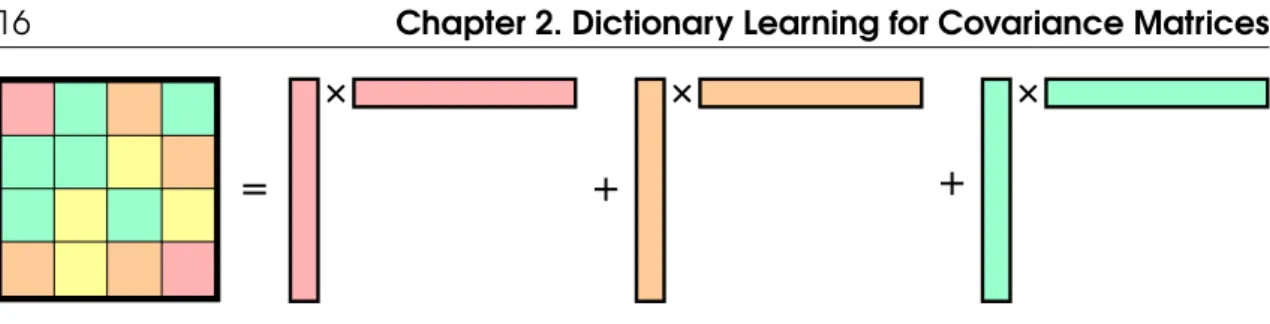
(16) Thèse de Daniele Calandriello, Lille 1, 2017. +. +. =. +. Chapter 2. Dictionary Learning for Covariance Matrices. 16. +. +. Figure 2.1: Dictionary Learning for Covariance Matrices 1. we can use I to represent D, 2. the dictionary’s size |I| is small and does not scale with n,. A dictionary is a generic collection of weighted atoms I := {(weight, atom)} = {(si , ai )}, where the atoms ai are arbitrary elements of Rd , and si are non-negative weights2 . The size of the dictionary |I| is the number of distinct atoms with a non-zero weight. We say that a dictionary I can be used to exactly represent dataset D when it is possible to exactly � si ai aTi as a weighted sum of the elements in reconstruct the covariance matrix XXT = the dictionary (see Fig. 2.1). If the dictionary correctly reconstructs XXT but its size does not scale with n (i.e., it is small ), we can use it in place of XXT to answer our machine learning questions (e.g., fit a linear model). Clearly the dictionary necessary to represent XXT is not unique, and many alternatives are possible, that differ in the choice of atoms and weights. We will now consider some options: Without learning. The simplest choice for a dictionary that needs to represent D is D itself, that is we do not change atoms or weights and set I = {(1, xi )}ni=1 . This �neither perfectly reconstructs D since ni=1 1xi xTi = XXT , but does not save any space.. Learn atoms.3 As soon as n > d, I = D is not the most succinct (in number of atoms) representation possible. Consider the thin Singular Value Decomposition of X = VΣUT and let r be the rank of X 1. V ∈ Rd×r contains the orthonormal left singular vectors vi ∈ Rd as columns, such that VT V = Ir and VVT is the projection on Im(X). 2. Σ : Rr×r is the diagonal matrix where [Σ]i,i = σi is the i-th singular value, and σr ≥ σr−1 ≥ · · · ≥ σ1 > 0. 3. U : Rn×r contains the orthonormal right singular vectors ui ∈ Rn as columns, such that Im(U) = Im(XT ).. Then we can rewrite T. T. T. T. T. T. XX = VΣU UΣ V VΣΣ V =. r �. σi2 vi viT. i=1. and use I = {1, σi vi } as a dictionary for D, replacing the atoms xi with σi vi . Clearly the number of atoms in the SVD-based dictionary is smaller than the one in the original dataset, but unfortunately when n is very large computing the SVD is prohibitively expensive. Learn weights but not atoms. This is the family of dictionaries I = {(si , xi )}ni=1 . When si = 1 for all i (i.e., I = D) we saw that this is not the most succinct representation 2. Since the matrix XXT is PSD, non-negative weights are sufficient for reconstruction. This approach is equivalent to learning both atoms and weights, since we can always rescale the learned atoms to include any necessary weight. 3. © 2017 Tous droits réservés.. lilliad.univ-lille.fr.

(17) Thèse de Daniele Calandriello, Lille 1, 2017. 2.1 Nyström in an Euclidean space: leverage score sampling. 17. possible, and there must be some redundancies that we can eliminate. A simple example of redundancy can be seen when xi and xi� are equal. In this case, we can simply remove xi� from� the dictionary setting si� = 0 and compensate by setting si = 2. � This leaves ni=1 si xi xTi = ni=1 xi xTi = XXT unchanged. In other words we can leave the atoms xi unchanged, but adapt the weights si to the data in order to reduce the number of non-zero weights and the size of the dictionary. While general dictionary learning consider the overall problem of jointly learning the weights and atoms, in the remainder of this thesis we will focus only on this last approach of selecting and reweighting a subset of D itself, sometime called sparse coding or sparse approximation. Given the selected subset, we can define the selection matrix S associated with a dictionary √ as S = Diag({ si }ni=1 ) ∈ Rn×n . Then XS is a Rd×n matrix where the atoms contained in I are properly reweighted so that XSST XT =. n �. si xi xTi .. i=1. Unfortunately (even when n > d) it is not always possible to find a subset of input samples xi that is strictly smaller than D and exactly reconstructs D. If we want to reduce the size of the dictionary we must incur in some approximation error. We will consider two metrics to quantify our approximation error. We present the first here, and postpone the second to Section 2.2.1. 2.1.1. Subspace approximation As we mentioned before, the covariance matrix XXT plays a central role in many linear problems, such as linear regression or PCA, that try to find the vector or vectors in a linear space that best fit the data collected. More formally, the solution to all of these problems must lie in Im(X) = Im(XXT ), and is computed using the spectral information contained in XXT , in the form of eigenvectors and eigenvalues. Therefore if the span and the spectrum of XSST X is close to that of XXT , we can use only the data contained in the dictionary to compute an accurate approximate solution. Chapters 4 and 5 will quantify more rigorously how an accurate dictionary translates into a good approximate solution, while we will now give our definition of accurate dictionaries. We begin by introducing the orthogonal projection matrix on Im(X) as a proxy for the spectrum of X, Definition 2.1 The orthogonal projection Π on Im(X) is defined as. Π = (XXT )+/2 XXT (XXT )+/2 =. n �. πi πTi ,. 2.1. i=1. � for a dictionary I with πi = (XXT )+/2 xi . The approximate orthogonal projection Π and its selection matrix S is defined as � = (XXT )+/2 XSST XT (XXT )+/2 = Π. n �. si πi πTi .. 2.2. i=1. � Note that Π = Id when X is full rank, and that we can also express Π = ri=1 vi viT , i.e., the SVD dictionary can represent Π using only r atoms, while the {πi }ni=1 dictionary. © 2017 Tous droits réservés.. lilliad.univ-lille.fr.

(18) Thèse de Daniele Calandriello, Lille 1, 2017. 18. Chapter 2. Dictionary Learning for Covariance Matrices. � is not the requires n atoms. Finally, note that the approximate orthogonal projection Π orthogonal projection on Im(XS) � �= ΠI := (XSST XT )+/2 XSST XT (XSST XT )+/2 . Π. � because we are not only interested in reconstructing the We chose this definition for Π T subspace spanned by XX , but we also want to reconstruct its defining spectral prop� is the right tool for the job, we use Definition 2.2 and Proposierties. To show that Π tion 2.1. n×n Definition 2.2 A dictionary I = {(si , xi )}n i=1 and its associated selection matrix S ∈ R are ε-accurate w.r.t. a matrix X if � = �(XXT )+/2 X(In − SST )XT (XXT )+/2 � ≤ ε �Π − Π�. 2.3. Proposition 2.1 — (Kelner and Levin, 2013).. �(XXT )+/2 (XXT − XSST XT )(XXT )+/2 � ≤ ε �. T. (1 − ε)XX � XSST XT � (1 + ε)XXT. 2.4. Due to the definition of Löwner PSD ordering, if the dictionary I is ε-accurate Proposition 2.1 guarantees that, for any a ∈ Rd , aT XSST XT a is at most a (1 ± ε) constant multiplicative error away from aT XXT a. Since aT XXT a = 0 only if a ∈ Ker(XXT ), this implies that Ker(XXT ) = Ker(XSST X), Im(XXT ) = Im(XSST X), and the dictionary perfectly reconstructs the projection Π Π = (XXT )+/2 XXT (XXT )+/2 = (XSST XT )+/2 XSST XT (XSST XT )+/2 = ΠI . We can also show that the spectrum of XXT is preserved. In particular, ε-accuracy and Proposition 2.1 implies that all eigenvalues of XXT are approximated by XSST XT up to the same constant factor. Therefore, ε-accuracy not only preserves the subspace that contains X, but also approximates well the importance of each direction in that subspace. As we will see this translates in stronger guarantees for complex problems such as PCA and regression. In addition, since XSST XT has to approximate at least r eigenvalues and eigenvectors, it is easy to see that an ε-accurate dictionary must contain at least r atoms (e.g., to approximate a diagonal matrix such as Ir , we need at least r atoms). Now that we defined an accuracy measure, there are many possible ways to try to find a dictionary and selection matrix S that satisfy it. Gradient descent. We can rewrite Eq. 2.3 as a function of the weights si as � � n �� T� (1 − s )π π min � i i i� � � {si }n i=1 i=1. A simple approach would be to use gradient descent mixed with an �-0 or �-1 penalty on the weights si to minimize this objective. Unfortunately computing the vectors πi requires O(nd2 ) time and is not efficient. Moreover computing a gradient w.r.t. n weights si , and repeating this operation at each step again makes the algorithm’s complexity scale poorly with n. Greedy choice with barrier function. Instead of performing expensive full gradient. © 2017 Tous droits réservés.. lilliad.univ-lille.fr.

(19) Thèse de Daniele Calandriello, Lille 1, 2017. 2.1 Nyström in an Euclidean space: leverage score sampling. 19. Algorithm 1 Nyström method Input: Budget q, set of probabilities {pi }ni=1 such that for all i 0 < pi ≤ 1 Output: I 1: Initialize I = ∅ 2: for i = {1, . . . , n} do 3: Draw the Binomial r.v.�qi ∼ B(pi , q) � 1 qi 4: If qt �= 0, add pi q , xi to I 5: end for updates, several papers (Batson et al., 2012; Silva et al., 2016) propose to use simpler greedy methods, providing increasingly stronger guarantees for these approaches. Given a partial dictionary, their strategy is to sequentially compute which would be the vector πi that would further the most the approximation goal while keeping the existing dictionary fixed. Batson et al., (2012) show that using appropriately constructed barrier functions to quantify the usefulness of each πi vector, it is possible to prove that this sequential approach generates an ε-accurate and in many cases optimally small dictionary. Unfortunately each step of this strategy requires solving a linear system in X and it is not computationally efficient, unless X satisfies stringent structural assumptions, e.g., when XXT is the Laplacian of a graph (Lee and Sun, 2015). Random sampling. A traditional (Williams and Seeger, 2001) and common heuristic to construct a dictionary is to build an unbiased estimator of Π choosing the weights with uniform sampling. In particular, we sample a small subset of q atoms uniformly at random (i.e., with probability p = 1/n), and set their weight to si = 1/(pq) = n/q. This strategy is simple, requires no knowledge of πi , and almost no computation. Unfortunately, it often fails to construct an ε-accurate dictionary (Bach, 2013). Nonetheless if we replace the data oblivious uniform distribution with a more accurate data adaptive distribution, we can improve our accuracy. In the next section we will focus on this family of sampling methods, and discuss how to find a good data adaptive distribution. 2.1.2. Nyström sampling In Section 2.1 we restricted our attention to dictionaries that select and reweight a subset of the input matrix. The Nyström method is a general name for all methods that choose this subset according to a random process. The blueprint for batch Nyström sampling is reported in Algorithm 1. The algorithm iterates over each atom xi and draws a Binomial random variable qi ∼ B(pi , q) containing q independent copies of a Bernoulli Ber(pi ). While we refer to qi as the number of copies of atom xi , Algorithm 1 does not explicitly add duplicate copies of xi to the dictionary I, but a single copy with weight p1i qqi . � Notice that traditionally Nyström sampling draws q( ni=1 pi ) samples without (Williams and Seeger, 2001) or� with (Alaoui and Mahoney, 2015) replacement from the multinomial distribution M({pi / ni=1 pi }). Algorithm 1 draws q samples from each of the n Binomials B(pi , q), which can be seen as a “Bernoulli with replacement”. On a statistical level this sampling scheme differs from Multinomial sampling in two aspects. �n The first �n difference is that the size of the dictionary |I| = q = i=1 qi is not fixed in advance to q( i=1 pi ) but� random and equal to �the number of non-zero weights contained in the dictionary |I| = ni=1 I{ p1i qqi �= 0} = ni=1 I{qi �= 0}. Nonetheless, we can bound w.h.p.. © 2017 Tous droits réservés.. lilliad.univ-lille.fr.

(20) Thèse de Daniele Calandriello, Lille 1, 2017. 20. Chapter 2. Dictionary Learning for Covariance Matrices. the final size of the dictionary to show that it is at most 3q(. �n. i=1 pi ).. Proposition 2.2 Given probabilities {pi } and budget q, let I be the dictionary generated. by Algorithm 1. Then � �� n �� n �� P |I| ≥ 3q pi pi . ≤ exp −q i=1. i=1. Proof sketch of Proposition 2.2. While the true size of the dictionary is the number of �n non-zero weights, it is easier to analyze the upper bound |I| ≤ i=1 qi , as if we assumed that all the copies included in the dictionaries belonged to different atoms, or we explicitly stored each copy of an atom separately. Then we can use a Hoeffding-like bound, proved in Proposition 2.13, to bound the sum of independent, non-identically distributed Binomials �n q . � i=1 i. The second difference is that, although in expectation both the number of drawn samples for � each atom (E[qi ] = qpi ) and in total (E[q] = q ni=1 pi ) match between the two approaches, our �sequential Binomial sampling is not equivalent (same distribution) as a series of q( ni=1 pi ) Multinomial draws with replacement4 . On an algorithmic level, unlike �n traditional Nyström, we do not need to explicitly compute the normalization constant i=1 pi to perform the sampling procedure. This will become useful in Section 2.2.2, where the pi will be computed starting from data. Other algorithm that use this Binomial sampling approach are present in the literature (Kelner and Levin, 2013), as well as variants that draw qi proportionally to an overestimated Bernoulli Ber(pi q) rather than a Binomial B(pi , q) (Cohen et al., 2015a; Cohen et al., 2015b; Cohen et al., 2016; Musco and Musco, 2017). It is easy to see that P(Ber(pi q) = 0) = 1 − pi q ≤ (1 − pi )q = P(B(pi , q) = 0), and drawing from the Binomial will produce smaller dictionaries. From the definition of sampling probabilities pi and weights p1i qqi we can see that the dictionary I is an unbiased estimator of D since 1 n n � � ✼ ✓ 1 E[q ] q p i i T T xi xTi = E[XSST XT ] = ✓ xi xi = XX . pi q p q i ✓ i=1. i=1. This holds for any valid set of probabilities pi and any q but it is easy to see that some choices are better than others. For example selecting extremely small pi for all i and q = 1 will almost certainly result in an empty (and very inaccurate) dictionary. From an accuracy � are close to their mean XXT perspective, we want to know when XSST XT , and in turn Π, and Π, or in other words when XSST XT concentrates. From a computational improvement perspective, we want to know when the generated dictionary I is small. Two factors impact these two quantities. The probabilities. The probabilities pi used to sample the Binomials tells us which atoms to choose and how many. More in general, the probability pi should � tell us how unique or redundant each pi encodes how many atoms overall are sample is, and the sum of these probabilities 4 In particular, drawing q elements from a Multinomial correspond�to the sequence of Binomial draws �n−2 q1 ∼ B(p1 , q), q2 |q1 ∼ B(p2 /(1 − p1 ), q − q1 ), . . . , qn−1 ∼ B(pn−1 /(1 − n−2 i=1 pi ), q − i=1 qi ). © 2017 Tous droits réservés.. lilliad.univ-lille.fr.

(21) Thèse de Daniele Calandriello, Lille 1, 2017. 2.1 Nyström in an Euclidean space: leverage score sampling. 21. necessary to represent the dataset. The concentration of XSST XT around its mean will be guided by how closely the distribution pi captures the true underlying redundancies. Remember from the previous section that we can find a small dictionary that accurately reconstruct the dataset because there are redundancies between samples. Consider the example dataset D = {x, x, x� , x� , x� } with two identical copies of x, three identical copies of x� , and xT x� = 0 orthogonal. The dictionary that perfectly reconstruct this dataset is {(2, x), (3, x� )} with minimal size 2. How would we set our probabilities in Algorithm 1 to generate this dictionary? � To obtain 2 and 3 as our weights, we set p1 = p2 = 1/2 and p3 = p4 = p5 = 1/3, with pi = 2 total number of needed atoms. This example also highlights why we need randomization: selecting greedily the two most unique atoms associated with the highest probabilities (x1 and x2 ) will not generate a good dictionary. The number of copies. The budget q tells us the extra budget we have to pay to compensate the intrinsic randomness induced by the random sampling, and any mistake in choosing the probability pi (mismatch between chosen pi and true redundancies). Take again the example D = {x, x, x� , x� , x� } with p1 = p2 = 1/2 and p3 = p4 = p5 = 1/3. If we set q = 1, simply due to the way q1 and q2 are randomly selected, we have a 1/4 possibility to generate a bad dictionary that does not contain x. Increasing q reduces the probability of this event happening. Similarly, if we underestimate the importance of a sample (e.g., set p1 = p2 = 1/4), increasing q will bring the final dictionary close to the mean no matter what kind of error we make. While increasing q helps with accuracy, we saw that our dictionary size increases as q, so raising it excessively might result in a very large dictionary that will not improve our computational complexity. 2.1.3. Uniform sampling To see an example of how the probabilities and budget q impact accuracy and dictionary size, we begin by considering uniform probabilities pi = 1/n. We will refer to Algorithm 1 using uniform probabilities as Uniform. Historically the first Nyström methods introduced in machine learning (Williams and Seeger, 2001) used uniform sampling, and it remains a popular choice for its conceptual simplicity and the fact that computing this distribution takes no computation at all. More recently, Bach, (2013) provided sufficient conditions under which uniform sampling generates an ε-accurate dictionary, using the dataset’s coherence to quantify the number of samples necessary. Definition 2.3 — (Drineas et al., 2012). Given a matrix X, the coherence µ of X is. µ = max �πi πTi � = max �πi �2 i=1,...,n. i=1,...,n. 2.5. Proposition 2.3 — (Bach, 2013, App. B1, Lem. 2). Consider an arbitrary matrix X ∈. � be defined according to Rd×n with xi as its i-th column and rank r. Let Π and Π. © 2017 Tous droits réservés.. lilliad.univ-lille.fr.

(22) Thèse de Daniele Calandriello, Lille 1, 2017. Chapter 2. Dictionary Learning for Covariance Matrices. 22. Definition 2.1. Let I be the dictionary generated by Algorithm 1. If pi = 1/n, with. �n. i=1 pi. q ≥ nµ. 4 log(2d/δ) , ε2. = 1, then for any 0 < ε < 1 and w.p.1 − δ. Accuracy: I is ε-accurate.. Space: the size of the dictionary is bounded by |I| ≤ 3q.. Proposition 2.3 tells us that to construct an ε-accurate dictionary, we should sample roughly O(nµ) atoms, which can correspond to almost the whole dataset when µ is close to 1. Unfortunately, estimating the coherence µ is a hard problem in itself (Drineas et al., 2012), therefore running uniform sampling with guarantees is not easy. As a solution, it is common in the Nyström literature to make an assumption of low coherence. Since the coherence µ is directly related to how much samples in the dataset are orthogonal with each other, Proposition 2.3 also gives us intuition on how uniform sampling can fail. For example, consider the case where a single sample xi is completely orthogonal to the others (µ = 1), and we try to use uniform probabilities in Algorithm 1 but set q to a constant (w.l.o.g. q = 1) to have a dictionary size that does not scale with n. Then the probability of not including the orthogonal sample is going to be roughly (1 − 1/n) ∼ 1. � ∼ 1 simply by testing And if we do not include the sample, it is easy to see that �Π − Π� T � i = 0 since these two matrices along the sample direction, where xi Πxi = xTi xi and xTi Πx xi is orthogonal to all other samples. Note that this problem will not happen with high probability only when a single sample is orthogonal. As an example, imagine that we have n1/2 vectors identical and orthogonal to the rest, we are still going to miss them with probability roughly (1 − 1/n1/2 ). This also is in line with our intuition of q as an extra budget to compensate inaccuracies in choosing pi . When the coherence is small, and no sample is orthogonal to the others, all samples look the same and have the same importance of roughly 1/n, making uniform sampling very accurate. But if the coherence is high, uniform probabilities are very likely to not correspond at all to the true underlying importance of each samples (they are chosen before even looking at the samples), and to concentrate we need a large number of copies q that potentially scales with n. To see how to remove this dependency on the coherence, let us first give a sketch of Proposition 2.3’s proof. The proof is based on the following general concentration for matrices, Proposition 2.4 — (Tropp, 2012, Theorem 1.6). Consider a sequence [Xj ] of independent. random symmetric matrices with dimension t. Assume that E[Xj ] = 0, �Xj � ≤ R, and � let Y = j Xj . Furthermore, assume that there exists σ > 0 that bounds the matrix variance statistic of the sum � E[Y 2 ]�2 ≤ σ 2 . Then � � ε2 /2 . P(�Y� ≥ ε) ≤ t exp − 2 σ + Rε/3. Proof sketch of Proposition 2.3. We provide a sketch of the proof here and include the full result in Section 2.3. Intuitively, the core of the proof consist in finding appropriate values for R and σ 2 to apply Proposition 2.4. In our case we use uniform sampling with probabilities pi = 1/n and the matrix we are. © 2017 Tous droits réservés.. lilliad.univ-lille.fr.

(23) Thèse de Daniele Calandriello, Lille 1, 2017. 2.1 Nyström in an Euclidean space: leverage score sampling interested in is Y = Π =. �n. i=1 πi πi . T. 23. We can show that. �πi �2 n maxi �πi �2 1 nµ = R := max = , q i pi q q �πi �2 n nµ 1 nµ σ 2 := max �Π� ≤ , �Π� = max �πi �2 �Π� ≤ q i pi q i q q satisfy the necessary conditions, and then apply the proposition. 2.1.4. �. Oracle leverage score sampling From the proof sketch of Proposition 2.3 we saw that the norms of the individual atoms �πi �2 = �(XXT )+/2 xi xTi (XXT )+/2 � plays a large role in bounding the range and variance of the random process induced by Algorithm 1. These quantities are well known in Statistics under the name of leverage scores. Definition 2.4 — (Drineas et al., 2012). Given a matrix X, the leverage score (LS) of. column xi ∈ X is. τi = �πi πTi � = �(XXT )+/2 xi xTi (XXT )+/2 � = xTi (XXT )+ xi .. 2.6. Furthermore, the sum of the leverage scores n � i=1. � � τi = Tr(Π) = Tr XXT (XXT )+ = Rank(XXT ) = r,. is equal to the rank of XXT . The leverage score τi intuitively captures how orthogonal xi is w.r.t. the rest of the samples X, and serves to rigorously measure what we so far called redundancy w.r.t. to preserving the spectrum of XXT . LSs have the following properties: • LSs are always smaller than 1. The maximum LS for sample xi is achieved when xi is orthogonal to all other samples: then xTi (XXT )+ xi = xTi (xi xTi )+ xi = 1. • LSs are always larger than 0. The minimum LS is achieved when xi is identical to all other samples (all samples are equal): then xTi (XXT )+ xi = xTi (nxi xTi )+ xi = 1/n. • The sum of the leverage scores captures the overall orthogonal directions contained in the data, making it equal to the rank of X. • The coherence of the matrix X is equal to the maximum LS (maxi τi ). Therefore, the low coherence assumption commonly used when applying uniform sampling is saying that no leverage score should be higher than the other, or alternatively that the leverage scores should be uniform. • Computing the LSs is computationally expensive, requiring nd2 operations to construct the XXT matrix. For simplicity we assume that an efficient oracle can compute them for us. In practice there are many efficient algorithms (Cohen et al., 2015a; Drineas et al., 2012) to approximate them in O(nd log(d)) or O(nnz(X) log(d) + d3 log(d)) time. Finally, note that the LS of sample xi is equal to the squared norm �πi �2 of the corresponding atom in Π. Intuitively, this means that samples with larger LS contribute more to the spectrum of Π. Since our goal is to reconstruct Π, it seems therefore reasonable to use LS as data adaptive probabilities pi in Algorithm 1 instead of the data oblivious probabilities. © 2017 Tous droits réservés.. lilliad.univ-lille.fr.

(24) Thèse de Daniele Calandriello, Lille 1, 2017. Chapter 2. Dictionary Learning for Covariance Matrices. 24. used in uniform sampling. The following proposition help us quantify how this help us in approximating Π. Proposition 2.5 — (Alaoui and Mahoney, 2015, App. A, Lem. 1). Consider an arbitrary. matrix A ∈ Rd×n with ai as its i-th column and assume maxi=1,...,n �ai �2 ≤ 1. Let I be the dictionary randomly generated by Algorithm 1 using probabilities pi ≥ �ai �2 . For any t > 0 we have � � qε2 /2 T T T 2.7 P(�AA − ASS A � ≥ ε ≤ 2d exp − (�AAT � + ε/3). Proof. The proof remains substantially the same as (Alaoui and Mahoney, 2015, Thm.2) up to two differences. (1) We consider the spectral norm � · � rather than the largest eigenvalue since in general AAT − ASST AT is not guaranteed to be PSD, and (2) we use our “Bernoulli with replacement” rather than Multinomial with replacement. As a sketch, the proof uses the same approach as Proposition 2.3, applying Proposition 2.4 to Π, but this time using pi ≥ �ai �2 instead of pi = 1/n. This lets us develop a tighter bound R :=. �ai �2 pi 1 1 1 max = max = , q i pi q i pi q. σ 2 :=. �ai �2 �AAT � �AAT � max , ≤ i q pi q. Intuitively, what this proposition tells us is that to preserve in spectral norm the sum of �n T T rank-1 matrices AA = i=1 ai ai , we want to sample more often matrices with � larger norm. Under the hood of the proof, this is because in the random sum ASST AT = ni=1 si ai aTi rank-1 matrices with larger norm cause larger variance, and sampling them more often help us to reduce the variance and concentrate around the expectation. � Noting that the LS are the norm of the columns of Π, we can instantly apply Proposition 2.5 to obtain Corollary 2.6 — Proposition 2.5, Proposition 2.13. Consider an arbitrary matrix X ∈ Rd×n. � be defined according to Definition 2.1, with xi as its i-th column and rank r. Let Π and Π and the LS τi according to Definition 2.4. Let I be the dictionary generated by Algorithm 1 run with parameters pi = τi , and. �n. i=1 pi. q≥. 4 log(4r/δ) , ε2. = r. Then for any 0 < ε < 1 and w.p.1 − δ. Accuracy: I is ε-accurate.. Space: the size of the dictionary is bounded by |I| ≤ 3qr. Proof of Corollary 2.6. The proof follows directly from Proposition 2.5. To replace the dependency on d with the dependency on r, it is sufficient to decompose Π before applying the concentration using the SVD decomposition � = �(XXT )+/2 X(In − SST )XT (XXT )+/2 � �Π − Π�. = �(ΣΣT )+/2 ΣUT (In − SST )UΣT (ΣΣT )+/2 �,. where ΣΣT ∈ Rr×r . This leaves unchanged the norms �ai �2 and all other quantities.. © 2017 Tous droits réservés.. �. lilliad.univ-lille.fr.

(25) Thèse de Daniele Calandriello, Lille 1, 2017. 2.2 Nyström in a RKHS: ridge leverage score sampling. 25. Algorithm 2 Nyström method in H Input: Budget q, set of probabilities {pi }ni=1 such that for all i 0 < pi ≤ 1 Output: I 1: Initialize I = ∅ 2: for i = {1, . . . , n} do 3: Draw the binomial r.v. qi ∼ B(p�i , q) � 1 qi 4: If qt �= 0, add pi q , φi = ϕ(xi ) to I 5: end for Note that this result was first derived by Drineas et al., (2008). With this corollary we have answered the question on which and how many atoms we need to sample to guarantee an accurate reconstruction of . We have finally satisfied the two goals of this section. For example, setting q = O(log(r)) gives us w.h.p. an ε-accurate dictionary that can reconstruct Π and XXT , with a total size smaller than O(r log(r)) that only scales with the actual rank of the problem, and independent from n. With this dictionary, we can solve downstream tasks in a time independent from n, making it feasible to scale to problems on very large datasets. Compared to uniform sampling, we do not need to assume a low coherence or select a large q to guarantee accuracy, because we will be actively looking for those orthogonal samples that made uniform sampling fail. In other words, our pi now capture much more closely our true underlying importance, and we can use a small logarithmic q because we only need to compensate the intrinsic randomness of the sampling process and not wrong probabilities. Moreover, the size of the dictionary automatically scales as qr, adapting to the rank and difficulty of the problem. Nonetheless the result is still not fully satisfactory. In particular, we have no way to automatically estimate r, so we typically resort to setting q = O(log(d)). In addition, two obvious shortcomings emerge from looking at the LS sampling approach Fast-decaying eigenvalues. Sometimes the rank of the matrix r is large and close to d, but only due to small numerical fluctuations. Or alternatively the smaller eigenvalues of XXT are negligible compared to the larger and we would like to ignore them. Large n, larger d. In many cases of interest d itself is also very large, and potentially larger than n. This is commonly the case when we project our point in some high dimensional space using tile-coding, wavelets, one-hot encodings or other combinatorial features. While these higher dimensional spaces have room for richer dictionaries, using LS to measure importance becomes vacuous, since it becomes possible for X to have n orthogonal vectors with τi = 1 and Algorithm 1 would simply keep all elements. In both of these cases, not only it is impossible to exactly reconstruct XXT using a dictionary smaller than n ≤ d, even ε approximation becomes impossible without storing all n input samples in the dictionary. In the next section, we will see how to further relax the approximation condition to tackle this setting, and how to generalize the LS to Regularized Leverage Scores.. 2.2. Nyström in a RKHS: ridge leverage score sampling To move from Rd to a Reproducing Kernel Hilbert Space H we must introduce some additional notation. First we do not restrict our samples xi to come from Rd anymore,. © 2017 Tous droits réservés.. lilliad.univ-lille.fr.

(26) Thèse de Daniele Calandriello, Lille 1, 2017. 26. Chapter 2. Dictionary Learning for Covariance Matrices. but make no assumption on the input space X . Then, given our dataset D of n arbitrarily chosen points5 xi ∈ X we use a feature map φ(·) : X → H to map the samples into the RKHS as φi = ϕ(xi ). In the remainder of the thesis, the points φi as will play the roles of points in a RKHS, samples from a dataset, columns of a map, or atoms in a dictionary, and we will refer to them accordingly depending on the context. To simplify the notation, we indicate with φTi φj the inner product �φi , φj �H in H. Also for simplicity and without loss of generality we assume that for all ϕ(xi ) the feature map ϕ induces a unit norm φTi φi = �φi �2 = 1. This is commonly satisfied in practice, for example by using Gaussian or cosine similarities for our H, or by normalizing the inputs xi in the Rd case. Alternatively, all our results can be extended to non-unit norm, with extra multiplicative terms of the form (maxi �φi �2 )/(mini �φi �2 ) appearing in space and time complexities. When evaluating computational costs, we also assume that computing the inner product φTi φj takes a time independent from n (i.e., constant). We also replace the matrix X with the map Φ : Rn → H composed by stacking together all points φi . To simplify again the notation, we indicate with ΦT : H → Rn its adjoint map. It is easy to see that the self-adjoint operator ΦΦT : H → H that replaces the covariance � matrix XXT remains PSD and it can again be expressed as ΦΦT = ni=1 φi φTi . The thin SVD of Φ = VΣUT must also be appropriately redefined. Let r be the rank of Φ, we have that 1. The projection matrix becomes a projection operator on Im(Φ) Π = (ΦΦT )+/2 ΦΦT (ΦΦT )+/2 = VVT based on the map V : Rr → H, where vi are the orthonormal eigenfunctions that span Im(Φ), such that VT V = Ir . Note that Π also acts as the identity for all vectors in Φ (Φ = ΠΦ) 2. Σ : Rr×r remains the diagonal matrix where [Σ]i,i = σi is the i-th singular value, and σr ≥ σr−1 ≥ · · · ≥ σ1 > 0 3. U : Rn×r remain the orthonormal vectors that span Im(ΦT ) Compared to the simpler leverage score sampling case in Rd , we have two new difficulties. First, we cannot store or manipulate directly the vectors φi , but only access them through inner products. Therefore it is not clear how to compute the LS φT (ΦΦT )+ φ. Second, when we choose our RKHS we prefer those with large dimension, because we want a rich space that can contain good solutions for our downstream task problems. As a consequence, it is very easy to end up constructing an H where Rank(Φ) = n. For example, using the Gaussian similarity the only way for the rank of the matrix to be smaller than the number of points is for some of the points to be exactly identical to each other. When the rank of the matrix is n, even if we could compute φT (ΦΦT )+ φ we would end up with all LS equal to 1, and the sampling would be meaningless. Nonetheless, in many cases the eigenvalues of ΦΦ decay very fast, or in other words only a few of the many (infinite) directions in H capture most of the information contained in Φ. 2.2.1. Regularized subspace approximation We can encode this intuition using a regularized projection, and a new (ε, γ)-accuracy definition. 5 i.e., we do not assume the points are sampled from a distribution, but since they are part of a dataset we still refer to them as samples.. © 2017 Tous droits réservés.. lilliad.univ-lille.fr.

(27) Thèse de Daniele Calandriello, Lille 1, 2017. 2.2 Nyström in a RKHS: ridge leverage score sampling. 27. Definition 2.5 The γ-regularized projection Γ on Im(Φ) is defined as T. Γ = (ΦΦ + γΠ). −1/2. T. T. ΦΦ (ΦΦ + γΠ). −1/2. =. n �. ψi ψTi ,. 2.8. i=1. � for a with ψi = (ΦΦT + γΠ)−1/2 φi . The approximate γ-regularized projection Γ dictionary I and its selection matrix S is defined as � = (ΦΦT + γΠ)−1/2 ΦSST ΦT (ΦΦT + γΠ)−1/2 = Γ. n �. si ψi ψTi .. 2.9. i=1. Definition 2.6 A dictionary I = {(si , φi )}n i=1 and its associated selection matrix S ∈. Rn×n are (ε, γ)-accurate w.r.t. a dataset Φ if. � = �(ΦΦT + γΠ)−1/2 Φ(In − SST )ΦT (ΦΦT + γΠ)−1/2 � ≤ ε �Γ − Γ�. 2.10. Associated with Definition 2.6 we have another reconstruction result Lemma 2.7. �(ΦΦT + γΠ)−1/2 (ΦΦT − ΦSST ΦT )(ΦΦT + γΠ)−1/2 � ≤ ε �. T. (1 − ε)ΦΦ − εγΠ � ΦSST ΦT � (1 + ε)ΦΦT + εγΠ. 2.11. Looking at the equation, we see that an (ε, γ)-accurate dictionary gives us the same (1 ± ε) multiplicative error guarantees of an ε-accurate dictionary, but also adds a εγ additive error. This means for example that only eigenvalues larger than εγ will be accurately reconstructed by the dictionary, and that the equivalence Ker(ΦΦT ) = Ker(ΦSST Φ) does not hold. Nonetheless, in many interesting problems (e.g., PCA, regularized regression) we were not interested in approximating the directions associated with smaller eigenvalues anyway, and as we will see in Chapter 4 and Chapter 5 this extra small error does influence too much the quality of the solutions computed on the dictionary. In exchange for this new mixed multiplicative-additive error, we can use Γ to define a generalization of the LS to this new d � n setting Definition 2.7 — (Alaoui and Mahoney, 2015). Given a map Φ : Rn → H, the γ-ridge. leverage score (RLS) of column i ∈ [n] is T. T. τi (γ) = φi (ΦΦ + γΠ). −1. φi =. n � j=1. σj2 σj2 + γ. [U]i,j .. 2.12. Furthermore, the effective dimension deff (γ) of the operator is defined as deff (γ) =. n � i=1. n � � � τi (γ) = Tr ΦΦT (ΦΦT + γΠ)−1 = i=1. σi2 . σi2 + γ. 2.13. Ridge leverage scores. The RLSs τi (γ) generalize the way LSs captures the overall orthogonality of a sample in the dataset, and LSs can be seen as a special case τi (0). In particular, the directions. © 2017 Tous droits réservés.. lilliad.univ-lille.fr.

(28) Thèse de Daniele Calandriello, Lille 1, 2017. 28. Chapter 2. Dictionary Learning for Covariance Matrices. associated with smaller eigenvalues are non-linearly penalized by the regularization γ, and being orthogonal along those direction will not make the sample important. Since the value of γ will be often clear from the context, we will refer to both LSs and RLSs as τi and only include the full notation τi (γ) when important. We can now look at two opposite cases to get an idea of how RLSs behave. When all samples are identical, the RLS of φi is at its minimum 0 ≤ φTi (ΦΦT + γΠ)−1 φi = φTi (nφφT + γΠ)−1 φi =. 1 φTi φi = , T nφi φi + γ n+γ. even lower than the corresponding lowest LS. When φi is orthogonal to all other samples its RLS is at its maximum 1 φT φi = ≤ 1. φTi (ΦΦT + γΠ)−1 φi = φTi (φi φTi + γΠ)−1 φi = T i φi φi + γ 1+γ But when we have many near-orthogonal samples the difference between LSs and RLSs emerge. While all the LSs would be very close to 1 (uniform sampling), looking at Eq. 2.12 we see that as γ grows, the RLSs are non-uniformly shrunk. In particular samples φi correlated with the larger eigenvalues of ΦΦ remain close to 1, while the ones correlated with smaller eigenvalues are shrunk (nonuniform sampling). For example a sample orthogonal to the others and fully aligned with the smallest non-zero eigenvalue λmin would be shrunk by roughly a λmin /γ factor. In the linear case where ϕ(·) : X → Rd (φi = xi ), the RLS can be explicitly computed as xTi (XXT + γId )−1 xi (Cohen et al., 2015b; Cohen et al., 2016). In the general H setting, to compute RLS in practice we can use the following equality Lemma 2.8 — (Calandriello et al., 2017a). The RLSs can be reformulated as. φTi (ΦΦT + γΠ)−1 φi =. � 1� T φi φi − φTi Φ(ΦT Φ + γIn )−1 ΦT φi γ. 2.14. While evaluating Eq. 2.14 is now possible, since ΦT Φ ∈ Rn×n and ΦT φi ∈ Rn are real matrices and vectors, it is still to computationally expensive. Operations involving ΦT Φ comprise the dominant part of this cost: it takes O(n2 ) space and operations to construct and store it, O(n3 ) operations to invert (ΦT Φ + γIn )−1 , and O(n2 ) operations to compute each φTi Φ(ΦT Φ + γIn )−1 ΦT φi using the precomputed inverse. For now, we will assume that an efficient oracle can compute τi (γ) for us, and we postpone the implementation of such an oracle to Chapter 3. Ridge leverage scores are also known under a number of different names in Statistics, often appearing together with the Gaussian distribution. Consider the problem of Gaussian process regression (Rasmussen and Williams, 2005), where our function is drawn from a f ∼ GP (0, ϕ(x)T ϕ(x� )) with mean function 0 and covariance function induced by ϕ(·). The target variables are generated as yi = f (xi ) + �i , with �i drawn i.i.d. from N (0, 1). Then, after drawing n samples the posterior variance of a new point x∗ w.r.t. the sample is σn (x∗ ) = φT∗ φ∗ − φ∗ Φ(ΦT Φ + In )−1 ΦT φ∗ .. This is almost equivalent to computing the RLS of φ∗ w.r.t. Φ using the reformulation from Lemma 2.8. The only difference is that φ∗ is not included in the inverse, or in other words that we compute the RLS w.r.t. Φ rather than w.r.t. [Φ, φ∗ ] as we did so far. Taking this interpretation, Srinivas et al., (2010) shows that for Gaussian processes, points that maximize RLSs (large variance) also approximately maximize the information gain I({yi }|f ) (Cover and Thomas, 2012).. © 2017 Tous droits réservés.. lilliad.univ-lille.fr.