Mod´
elisation de l’int´
egration des entr´
ees
synaptiques excitatrices chez les cellules
thalamocorticales
M´emoire pr´esent´e
`a la Facult´e des ´etudes sup´erieures de l’Universit´e Laval dans le cadre du programme de maˆıtrise en physique pour l’obtention du grade de maˆıtre `es sciences (M.Sc.)
FACULT´E DES SCIENCES ET DE G´ENIE UNIVERSIT´E LAVAL
QU´EBEC
2011
c
Les cellules thalamocorticales (TC) du noyau ventro-post´ero-lat´eral (VPL) du thala-mus relayent l’information du syst`eme somatosensoriel (synapses excitatrices lemnis-cales aux dendrites proximaux) `a la r´egion correspondante du cortex, mais re¸coivent ´egalement en r´etro-propagation des projections du cortex (synapses excitatrices cor-ticothalamiques aux dendrites distaux). Afin d’´etudier l’int´egration synaptique aux diff´erentes parties de la cellule TC, nous avons bˆati un mod`ele multi-compartimental `a partir de reconstructions tridimensionnelles de cellules du noyau VPL, ce qui consiste en une discr´etisation spatiale des dendrites en une multitude de segments associ´es `a des circuits RC interconnect´es. Nous avons pu d´egager quantitativement l’impact de la g´eom´etrie cellulaire (taille d’arborisation et diam`etre dendritique) sur l’amplitude et sur la dur´ee des r´eponses au soma. Nous avons par la suite compar´e l’int´egration synap-tique pour diff´erentes distributions des entr´ees aux dendrites proximaux et distaux et sous diff´erentes conditions de courants intrins`eques et de potentiel membranaire. Dans tous les cas, la sommation des entr´ees proximales induisait une r´eponse ind´ependante de la distribution, alors que la r´eponse aux entr´ees distales saturait lorsqu’elles ´etaient localis´ees aux mˆemes branches. Nos r´esultats ont permis d’apporter une explication physiologique au patron d’organisation synaptique chez les cellules TC.
Thalamocortical (TC) cells from the ventroposterolateral (VPL) nucleus of the thalamus relay the somatosensory inputs (excitatory lemniscal synapses at proximal dendrites) to the corresponding cortical area, but also receive feedback excitatory inputs from the cortex (corticothalamic synapses at distal dendrites). The goal of this study was to compare the synaptic integration of inputs coming to proximal vs. distal dendrites. A multicompartmental model was drawn from fully reconstructed cells of the VPL nucleus. Dendrites were spatially discretized in multiple segments associated to interconnected RC circuits. We were able to characterize the impact of neuronal size and dendritic diameter on the amplitude and on the time course of the somatic response. We also compared the synaptic integration for different distributions of proximal or distal inputs under different conditions of membrane potential and active properties. In all cases, the summation of proximal inputs was independent of their distribution, while the response induced by distal inputs saturated when those inputs were located at the same branches. The results obtained in this study suggest a physiological explanation of the synaptic pattern at TC cells.
The following thesis contains the most important results obtained during my Master degree, which began in May 2009, as well as a detailed introduction and a brief con-clusion. The first part of the introduction contains basic notions of neurobiology that are necessary for a full understanding of the study. It is written for the physicist that would present some interest in neuroscience. To put the outcome of the study into an interesting perspective, a description of the thalamocortical system and of thalamocor-tical cells themselves is included. The next part of the introduction describes the model used. Finally, a brief overview of the numerical techniques underlying the simulations is given.
The results presented in this thesis are grouped into an article that is not yet submit-ted to a journal. It is the product of a collaboration with my two supervisors, the Dr. Helmut Kr¨oger, my principal supervisor, and the Dr. Igor Timofeev, my cosupervisor. Since I was the main investigator in this study, my name appears first on the article. I worked on the modeling and the programming parts and I achieved all the simulations and analyzed the data. Along with Dr. Timofeev, I participated in the writing of the article. My two supervisors provided the direction of the project and fruitful advice during the study. They were able to identify weaknesses in my work and to help me to solve the problems encountered. Note that part of those results or other results have been presented in numerous local, national or international conferences. Results and their implications are summarized in the conclusion.
I would like to thank both Dr. Kr¨oger and Dr. Timofeev for giving me a place of choice in their respective research groups. I would also like to thank my colleagues in both of those groups: Reza Zomorrodi, Jean-Fran¸cois Laprise and Ahmad Hosseinizadeh in the theoretical and computational Physics group, Sylvain Chauvette, Jos´ee Seigneur, Reza Zomorrodi, Maxime Lemieux, Courtney Pinard, Laszlo Grand, Tianyu Wang, Maxim Sheroziya, Mathieu Blais-D’Amours, Souma¨ıa Boubou and Sergiu Ftomov at the Centre de recherche Universit´e Laval Robert-Giffard. Despite rather absent di-rect scientific collaborations with the groups members, I met outstanding people and
built indestructible friendships. I am glad to continue my Ph. D. studies under the supervision of Dr. Timofeev and to work in such a great scientific environment.
I want to thank Dr. Andr´e Longtin and Dr. Yves De Koninck, who kindly agreed to evaluate this thesis, as well as Dr. Louis J. Dub´e for his great help and support during the last steps of the Master degree.
Last but not least, I would like to thank my close friends and the members of my family for their endless support during this finite, but long process. Most of them do not work in science and I believe that the interaction with such good friends and family members is crucial for the sanity of a scientist.
Finally, I wish full recovery to my supervisor, Dr. Helmut Kr¨oger, who suffered from a severe stroke last summer. He is a great physicist and teacher, but is also open minded to other fields of science, especially neuroscience. For those reasons he has all my admiration.
What I cannot create, I do not understand. -Richard P. Feynman
R´esum´e ii Abstract iii Foreword iv Contents vii List of Figures ix List of Tables xi
List of abbreviations xii
1 Introduction 1
1.1 The physiological context . . . 1
1.1.1 Some basic concepts . . . 1
1.1.2 The thalamocortical network . . . 8
1.1.3 The thalamocortical unit . . . 11
1.1.4 Thalamocortical oscillations . . . 15
1.2 Modeling biophysical processes . . . 19
1.2.1 The cable theory . . . 19
1.2.2 The compartmental model . . . 26
1.2.3 Modeling active membrane properties of thalamocortical cells . 29 1.3 Numerical simulations under the NEURON simulation environment . . 34
1.3.1 Temporal discretization . . . 34
1.3.2 Spatial discretization . . . 35
2 Integration of excitatory synaptic inputs in dendritic trees of thalam-ocortical neurons 37 2.1 R´esum´e . . . 38
2.2 Abstract . . . 38
2.3 Introduction . . . 39
2.4.1 Multicompartmental model . . . 40
2.4.2 Mean dendritic diameter . . . 41
2.4.3 Synaptic current and distributions of synaptic sites . . . 42
2.4.4 Statistical analysis . . . 43
2.5 Results . . . 43
2.5.1 Basic electrophysiological features . . . 43
2.5.2 Impact of the dendritic diameter on neuronal responses . . . 47
2.5.3 Linear vs. sublinear summation of fast excitatory synaptic po-tentials . . . 48
2.5.4 Centripetal vs. radial distributions of synaptic sites . . . 54
2.5.5 Effects of active dendrites and synaptic distributions on somatic responses . . . 57
2.5.6 Patterns of organization of synaptic contacts . . . 59
2.5.7 Threshold number of synaptic sites needed to elicit a somatic action potential . . . 61
2.6 Discussion . . . 64
3 Conclusion 67
1.1 Basic concepts. . . 3
1.2 Current-voltage relationships [1,2]. . . 4
1.3 Different states of Na+ and K+ channels for action potential generation. 7 1.4 Structures and specific pathways of sensory systems. Modified from [3]. 10 1.5 Thalamocortical circuitry and patterns of the slow oscillation in anaes-thetized cats [4]. . . 11
1.6 8 reconstructed neurons from the VPL nucleus. . . 12
1.7 Ascending somatosensory pathways. Modified from [3]. . . 13
1.8 Intrinsic electrophysiological properties of thalamocortical neurons [4]. . 15
1.9 Thalamic delta oscillation [4]. . . 17
1.10 Spindle activity [4]. . . 18
1.11 Cable theory. . . 20
1.12 Voltage spread in cables for different boundary conditions. Modified from [5]. . . 24
1.13 Compartmental modeling. . . 26
1.14 General form of a single compartment. . . 28
1.15 Active compartments. . . 34
2.1 Propagation of an evoked EPSP. . . 44
2.2 Mean diameter vs. distance to the cell body in 4 thalamocortical cells. 47 2.3 Dependence of somatic responses on the dendritic diameter in 4 thalam-ocortical cells. . . 49
2.4 Linear and sublinear summation of fast EPSPs in cell 1. . . 51
2.5 Linear and sublinear summation of fast EPSPs in cell 4. . . 52
2.6 Linear and sublinear summation of fast EPSPs in cell 6. . . 53
2.7 Dendritic integration in cell 1. . . 55
2.8 Dendritic integration in cell 6. . . 56
2.9 Dependence of the amplitude of somatic responses on the distribution of synapses (centripetal vs. radial) and on the activity of intrinsic currents. 58 2.10 Attenuation of synaptic responses propagating toward soma depends on dendritic path and branching point morphology. . . 60
2.11 Somatic responses of TC neurons to the activation of synapses with dif-ferent patterns of distribution. . . 62
2.12 Minimal number of synapses required to elicit an action potential in TC neurons. . . 63
2.1 Electrophysiological features. Proximal stimulus (60 µm). . . 46
AMPA α-amino-hydroxy-5-methyl-4-isoxazolepropionic acid CNS Central nervous system
EPSP Excitatory postsynaptic potential FPP fast pre-potential
FWHM Full width at half maximum GABA γ-aminobutyric acid
GHK Goldman-Hodgkin-Katz
GR Geometrical ratio
IN Interneuron
IPSP Inhibitory postsynaptic potential LTS Low-threshold spike
NMDA N -methyl-D-aspartate
ODE Ordinary differential equation PDE Partial differential equation PNS Peripheral nervous system PSC Postsynaptic current PSP Postsynaptic potential PY Pyramidal RE Reticular TC Thalamocortical VL Ventral lateral VP Ventral posterior VPL Ventroposterolateral
Introduction
1.1
The physiological context
1.1.1
Some basic concepts
The brain is one of the two components of the central nervous system (CNS), the other being the spinal cord. The CNS integrates the information coming from the peripheral nervous system (PNS). The nervous system contains two types of cells: neurons and glial cells. 100 billion neurons are present in the human brain. They are electrically excitable due to various complex ionic channels, ion pumps and synaptic receptors embedded in their plasma membrane. In contrast, glial cells are not electrically excitable, but are extremely important in maintaining the brain homeostasis and regulating the synaptic transmission. Some of them, the Schwann cells in the PNS and the oligodendrocytes in the CNS, also ensure a fast propagation of action potentials by forming myelin sheaths insulating the axon of neurons.
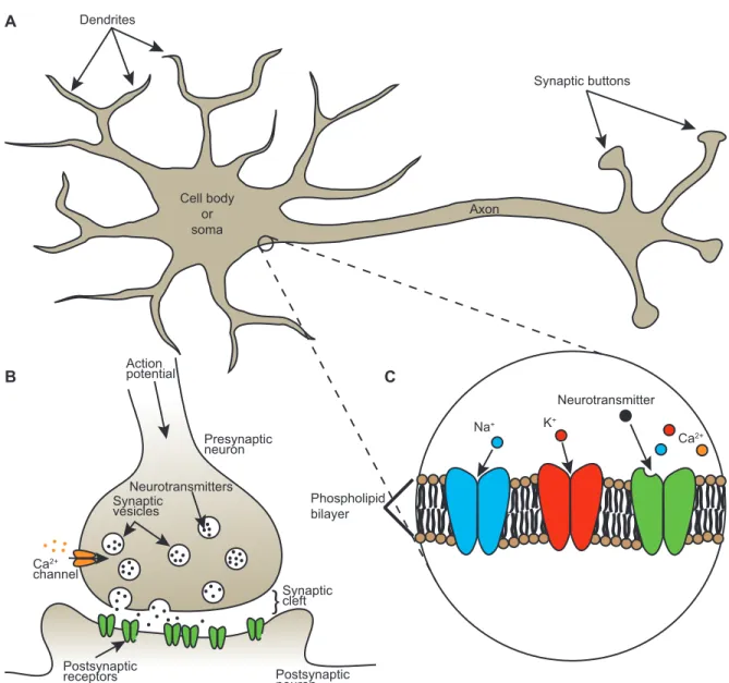
Neurons consist in three main parts (Fig. 1.1A). The dendrites receive chemical or electrical signals from other neuronal cells. The cell body or soma is the center of integration of information. Finally, the axon transmits this information to other cells. This transmission is achieved by the action potential, a fast high-voltage signal pro-duced at the soma when the cell is excited above a threshold called the firing threshold. The action potential propagates into the axon toward the synaptic contacts. Synapses constitute the connections between neurons and thus underlie all neuronal communica-tions. In other words, a synapse is the junction between the axon of a presynaptic cell, or more precisely a synaptic button at the end of the axon, and a dendrite of a
post-synaptic cell (Fig. 1.1B). Connections at the postsynaptic cell are typically established at protrusions emerging from the dendritic shaft called dendritic spines. The space between the presynaptic button and the postynaptic membrane is called the synaptic cleft. Neurotransmitters are released in that cleft via the release sites of the presynaptic neuron. They are captured by receptors at the postsynaptic neuron and a postsynap-tic response is induced. The plasma membrane of a neuron consists of a phospholipid bilayer, i.e. two layers of counteroriented lipid molecules. The intracellular medium or the cytoplasm is negatively charged compared to the extracellular medium. The difference in potential between the intracellular and extracellular media is simply called the membrane potential (Vm). Various proteins establishing multiple types of channels
that control in part the flow of ions and regulate the membrane potential are embedded in the phospholipid bilayer (Fig. 1.1C). Particularly important ions are K+, Na+, Cl−
and Ca2+. Most channels are said to be specific. For example, Ca2+ ions flow across
channels that are permeable to Ca2+ ions, but not across channels only permeable to
K+. Ions tend to move down their concentration gradient, but this movement changes
the distribution of charges and causes a voltage gradient or an electrostatic force that can act against the initial flow. When a channel is open, ions specific to that channel are allowed to flow from one side of the membrane to the other, the direction depending on the concentration and voltage gradients. When both phenomena are balanced, the net current across the membrane is zero and ions are in a dynamic equilibrium. The mem-brane potential value at which it occurs is the equilibrium memmem-brane potential Eion. It
thus depends on intracellular [ion]in and extracellular [ion]ext concentrations, but also
on the temperature T of the environment and on the valence z of ions. For a channel permeable to only one specific ion, Eion can be evaluated according to thermodynamics
by the Nernst equation:
Eion =
RT
zF ln([ion]in/[ion]ext), (1.1)
where R is the gas constant (8.314 J/K·mol) and F the Faraday’s constant (96 485 C/mol). This voltage level is also referred to as the ionic reversal potential. For Vm > Eion, positive ions flow from the inside of the cell to the extracellular space, while
for Vm < Eion, the direction is reversed. When different species of ions are present
in the membrane, Eq. (1.1) can be generalized to the Goldman-Hodgkin-Katz (GHK) equation:
Vrest =
RT F ln
!
PK+[K+]ext+ PNa+[Na+]ext+ PCl−[Cl−]in
PK+[K+]in+ PNa+[Na+]in+ PCl−[Cl−]ext
"
, (1.2)
where Pion is the permeability associated to a specific ion (usually in cm/s). The
Cl− concentrations are inverted in Eq. (1.2) compared to K+ and Na+ concentrations
because of the negative valence of Cl− ions. This expression provides the steady state value of Vm or the resting membrane potential Vrest. Vrest lies between -40 and -90 mV
Synaptic buttons Axon Cell body or soma Dendrites Ca2+ channel Postsynaptic receptors Postsynaptic neuron Presynaptic neuron Synaptic vesicles Neurotransmitters
}
Synaptic cleft Action potential A B Phospholipid bilayer Na+ K+ Neurotransmitter Ca2+ CFigure 1.1: Basic concepts. A, Schematic representation of a neuron. B, Synapse. C, Phospholipid bilayer with embedded channels.
A
B
Figure 1.2: Current-voltage relationships. A, Current-voltage relationship of a single nicotinic ACh-activated ionic channel for NH+4 (") and Li+ (#). The recordings were obtained from voltage-clamp
experiments on clonal BC3H-1 mouse muscle cells [2]. B, Current-voltage relationship for a single Ca2+-dependent K+channel. The recordings were obtained from voltage-clamp experiments on bovine
chromaffin cells [1]. Vertical axis: current, 8 pA per box. Horizontal axis: membrane potential (mV).
completely at rest due to constantly active neurons. The amplitude of the different currents taken into account in Eq. (1.2) can be described by Ohm’s law:
iion = gion(Vm− Eion), (1.3)
where gion is the ionic conductance density (usually in mS/cm2) and is a measure of the
channel density at the membrane. For ionic currents, iion and gion are simply referred
to as the ionic current and conductance, respectively, by keeping in mind that they represent the density of those quantities. Eq. (1.3) implies a linear current-voltage relationship for an open channel (Fig. 1.2A).
The GHK equation could technically include more than three different species of ions. However, other ions like Ca2+, despite a possibly crucial role in neuronal functions,
have intracellular and extracellular concentrations that are much lower than K+, Na+
and Cl− concentrations and can thus be neglected in Eq. (1.2). Furthermore, for highly
unbalanced intracellular vs. extracellular concentrations, Nernst, GHK and Ohm’s law equations are not accurate. In such case and for large variations of Vm, ions hardly
move against their concentration gradient. As a result, instead of being linear, the current-voltage relationship saturates for large variations of Vm (Fig. 1.2B). This is
particularly true for Ca2+ currents, the intracellular concentration being ∼10000 times
weaker than the extracellular concentration.
Channels possess sensors that react either to voltage variations for voltage-gated channels or to the presence of specific molecules in their environment for ligand-gated channels. Note that these classes are not exclusive. For a channel to open, sensors must react to their environment. For that reason, the openings and closings are stochastic processes. However, considering the whole population of channels at the membrane, one can describe the transition from one state to another as a smooth process. Note that most channels are also time-dependent. A particular type of ionic channels are the leakage channels that mediate the leak current. This current is considered as a passive property of the membrane since the channels opening does not depend on Vm or on
binding molecules. It is mainly responsible for the value of Vrest. Other types of current
are considered as active properties.
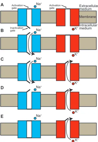
Channels are pores in the membrane that have one or two kinds of gates that are either activated, deactivated, inactivated or deinactivated. To let the current flow through it, a channel described by the two gates model must have both its activation and inactivation gates open. In such case the channel is activated and deinactivated. Some types of channels are only described by activation gates and do not inactivate or deinactivate. They allow ions to move across the membrane if they are activated, and block ions if they are deactivated. Consider the most important set of currents, i.e. the Na+ and K+currents responsible for the generation of action potentials. When
the membrane at the soma is sufficiently depolarized by cooperating effects of synaptic events and/or intrinsic currents, Vm reaches a threshold value (Vth) where specific Na+
channels are activated. Vth is referred to as the firing threshold. The highly increased
permeability to Na+ ions and the high driving force due to a positive reversal potential
of the Na+ current produce a strong and fast depolarization (> 60 mV in amplitude).
The generation of an action potential is an all-or-none process since its time course and its amplitude are independent on the stimulation, as long as it is strong enough to reach the firing threshold. However, this depolarization also activates channels of an outward persistent K+current that acts against the effect of Na+ions. In the meantime,
Na+channels are also inactivated. Given those two mechanisms, the membrane quickly
states of Na+ and K+ channels during the action potential are shown in Fig. 1.3. Note
that because K+ channels are slowly deactivated when the membrane is repolarized, V m
goes slightly below Vrestfor some time after an action potential has been generated. This
is the afterhyperpolarization phase. Note also that due to both the slowly deactivating K+ and the slowly deinactivating Na+ channels, there is a refractory period during
which another action potential cannot be generated.
When the propagating action potential reaches the end of the axon where are lo-calized synaptic buttons, the high depolarization applied on the membrane activates high-threshold Ca2+ channels. The Ca2+ ions crossing the membrane interact with
synaptic vesicles that contains neurotransmitters. The vesicles merge with the mem-brane at the synaptic buttons and neurotransmitters are released in the synaptic cleft. Those neurotransmitters eventually bind to postsynaptic receptors. Receptors are an-other type of proteins embedded in the plasma membrane. When neurotransmitters bind to these receptors, channels open, the membrane permeability is increased and specific ions are allowed to enter channels. This current produces a synaptic response, i.e. a transient change in the local Vm or a postsynaptic potential (PSP). Receptors
that bear their own channels are called ionotropic receptors. They are thus ligand-gated channels. Another family of receptors is the family of metabotropic receptors. They do not include ionic channels in their structure, but act indirectly on neighboring channels via intermediate molecules called G-proteins.
Neurotransmitters bind to specific receptors. Most common neurotransmitters or at least the most pertinent for the present study are the glutamate and the γ-aminobutyric acid (GABA) that binds to glutamatergic and GABAergic receptors, respectively. Synapses can be either excitatory or inhibitory, so they can depolarize or hyperpolarize the post-synaptic cell, respectively. Synapses that depolarize the postpost-synaptic cell and increase the probability of generating an action potential trigger excitatory postsynaptic poten-tials (EPSPs), while synapses that hyperpolarize the cell trigger inhibitory postsynaptic potentials (IPSPs). The α-amino-hydroxy-5-methyl-4-isoxazolepropionic acid (AMPA) and the N -methyl-D-aspartate (NMDA) receptors are glutamatergic receptors and me-diate EPSPs. GABAergic receptors such as GABAa and GABAb receptors induce
IPSPs at the postsynaptic membrane.
The amplitude of the postsynaptic current (PSC) isyncan be described by an ohmic
relation:
isyn = gsyn(t)(Vm− Esyn), (1.4)
where gsyn(t) is the synaptic conductance and Esyn is the reversal potential of the
synaptic current. Note that the conductance depends on time. Typically, ionotropic receptors promote a fast time course for PSCs or PSPs (e.g. AMPA-, NMDA- and
Na+ K+ Na+ K+ K+ K+ K+ Na+ Na+ Na+ Intracellular medium Extracellular medium Membrane A B C D E Activation gate Inactivation gate Activation gate
Figure 1.3: Different states of Na+ and K+channels for action potential generation. A, At rest, both
the Na+ and the K+ channels are deactivated. The inactivation gates of Na+ channels are open. B,
When the soma is depolarized to the firing threshold, the activation gates of Na+ channels open and
Na+ ions can cross the membrane from the outside of the cell to the inside. C, In the meantime, K+ channels are activated and an outward K+current is induced. D, Na+ channels are then inactivated.
The combined effect of the outward K+ current and the inactivation of Na+ channels produces a
fast repolarization toward the resting value of the membrane potential. E, The K+ channels slowly
deactivate after the repolarization, i.e. the channels stay open for some time. This slow deactivation causes the membrane potential to go slightly below its resting value for some time. This is the afterhyperpolarization phase.
GABAa-receptor-mediated PSPs) while a slow time course of the postsynaptic response
is associated to metabotropic receptors (e.g. GABAb-receptor-mediated IPSPs) due to
the indirect channel activation. However, due to different intrinsic kinetics, the NMDA-receptor-mediated current has a much slower time course than the AMPA type. The reversal potential is around 0 mV for typical excitatory synapses like AMPA- and NMDA-receptor-mediated synapses. Relation (1.4) already points out an important characteristic of the synaptic current. In the case of excitatory synapses, an already de-polarized membrane at the time of a synaptic event implies a reduced driving potential (Vm− Esyn) and thus a reduced synaptic current. This effect will have a major impact
on the synaptic integration since closely localized events will destructively interfere in that they will reduce each other’s driving potential for the synaptic current.
Chemical synapses formed between presynaptic axons and postsynaptic dendrites are stereotypical. However, one should note that synapses may also be formed between dendrites of presynaptic and postsynaptic neurons, as encountered between mitral and granule cells in the olfactory bulb, but also between axons. We will not discuss those dendro-dendritic and axo-axonic synapses here and will consider this issue as an excep-tion. Because they are much less present than chemical synapses, electrical synapses will also be ignored for the purpose of this study. Finally, other molecules embedded in the membrane form active transporters for ions called ion pumps. Their role is mainly to regulate the concentration and voltage gradients by acting directly against electrical and chemical forces. The information contained in this subsection and more can be found in textbooks [3,6].
1.1.2
The thalamocortical network
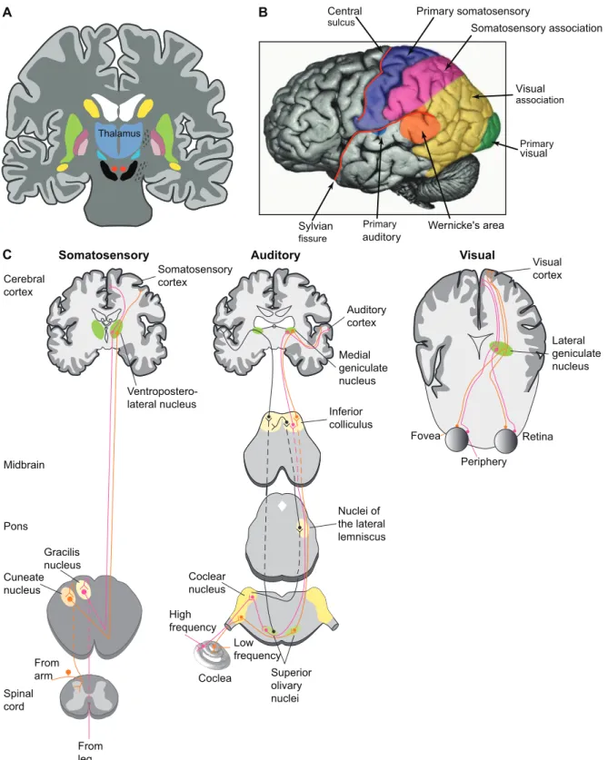
Located near the center of the brain (Fig. 1.4A), the thalamus relays the sensory infor-mation from the periphery to the neocortex via the TC cells, as well as the descending motor information to the neocortex. TC cells are also called thalamic relay neurons due to this relay function. The thalamus is thus the last station of the peripheral infor-mation before it reaches the cortex. For that reason it also plays a gating role for the sensory evoked inputs for the different states of vigilance encountered during wake and sleep. During sleep, the thalamus strongly reduces the relay of peripheral inputs to the cortex [7–10]. This is the consequence of a hyperpolarized membrane which is then far from the firing threshold [11]. This hyperpolarization is itself due to a reduced effect of the cholinergic inputs during sleep [12–14].
The thalamus can be divided in the dorsal thalamus and the ventral thalamus. The dorsal thalamus contains the TC cells, as well as some GABAergic interneurons
(INs) that inhibits TC cells. INs typically account for 25-30% of the population of the dorsal thalamus in cats, monkeys and humans brains [15–24], but are nearly absent in rodents [25–28]. The ventral thalamus forms a shell-like structure above the dorsal thalamus and is mainly composed of the thalamic reticular nucleus, which exclusively contains GABAergic reticular (RE) cells that inhibit thalamic relay nuclei. The zona incerta, the ventral lateral geniculate nucleus and the nucleus of the field of Forel are also a part of the ventral thalamus and may contain TC cells, but this is rather an exception. We can divide the dorsal thalamus in different nuclei, the majority of these nuclei being specific to a given sensory system and projecting to its corresponding cortical region (Fig. 1.4B, C). For example, visual stimuli are transmitted to the thalamus via the optic tract that connects to the dorsal lateral geniculate nucleus (first order) and the pulvinar (higher order). That visual information is then sent to the primary visual cortex in the occipital lobe. The only sensory system that does not require a thalamic gating is the olfactory system, which is also known to be the oldest sensory system. Some thalamocortical projections are non-specific, i.e. there are thalamic nuclei that send axons to different cortical fields. This is the case for intralaminar nuclei [29]. Subthalamic inputs of a common tract may also innervate various nuclei, like the spinothalamic tract that projects to both the ventral posterior (VP, sensory inputs) nucleus and the ventral lateral (VL, motor inputs) nucleus [30]. However, the lemniscal and the cerebellothalamic fibers connect exclusively to the VP and the VL nuclei, respectively.
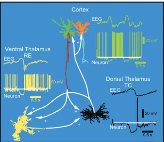
The thalamocortical system consists of the thalamus and the cortex interconnected into a loop (Fig. 1.5). A glutamatergic TC neuron innervates numerous neocortical neurons (mainly from the layer IV), but also receives feedback excitatory inputs from descending corticothalamic fibers arising from the corresponding cortical region (mainly from the layer VI). The main target of TC neurons are the spiny stellate neurons, but they also innervate cortical pyramidal (PY) neurons and in much lesser extent the aspiny interneurons (reviewed in [31]). Cortical projections to TC cells are made by PY neurons. Both thalamocortical and corticothalamic axons send collaterals to the reticular nucleus thus including RE cells in the recurrent thalamocortical network and establishing an excitation-inhibition loop between the dorsal and the ventral thalamus. The multiple thalamic relay nuclei of the dorsal thalamus constitutes the main gate to the cortex to specific ascending sensory inputs from the medial lemniscus, the optic tract, the brachium of the interior collicus, the ansa lenticularis and the brachium conjuctivum. TC neurons, as well as RE neurons, also receive non-specific inputs from the brainstem modulatory systems (noradrenergic, serotoninergic, cholinergic, etc.), which are important in modulating and regulating the different states of vigilance. More precisely, those inputs are mainly responsible of the blockade of K+channels during the
Thalamus
Sylvian
fissure
Central
sulcus Primary somatosensorySomatosensory association
Primary
auditory Wernicke's area
Primary
visual Visual
association
A B
Somatosensory Auditory Visual
Midbrain Ventropostero-lateral nucleus Pons Gracilis nucleus Cuneate nucleus Spinal cord From arm From leg Inferior colliculus Nuclei of the lateral lemniscus Coclear nucleus High frequency Coclea Low frequency Superior olivary nuclei Fovea Periphery Retina Cerebral cortex Somatosensory cortex Auditory cortex Medial geniculate nucleus Visual cortex Lateral geniculate nucleus C
Figure 1.4: Structures and specific pathways of sensory systems. A, Central position of the thalamus. B, Topological arrangement of the neocortex. C, Specific pathways of different sensory systems. Modified from [3].
50 mV 0.5 s 20 mV 0.5 s 0.5 s 20 mV Cortex Dorsal Thalamus TC Ventral Thalamus RE EEG Neuron EEG Neuron EEG Neuron + + -+ +
Figure 1.5: Thalamocortical circuitry and patterns of the slow oscillation in anaesthetized cats. Are shown a TC neuron from the VPL nucleus (black), a thalamic reticular cell (yellow), a cortical layer III pyramidal cell (green) and a cortical layer III interneuron (orange) [4].
state (reviewed in [13]). The gating function of TC cells and the recurrent organization of the thalamocortical system enable it to generate and to sustain spontaneous activity in the network during sleep, i.e. when the system is closed to peripheral information.
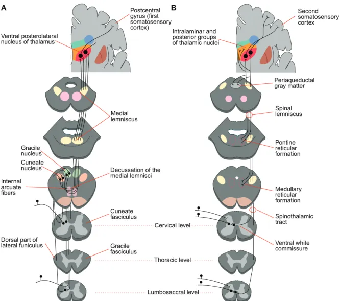
In the present study, we used 8 three-dimensional reconstructions of TC cells to build a model (Fig. 1.6). The reconstructed cells were from the VPL nucleus of the cat, which conveys the peripheral sensory inputs coming by the medial lemniscal pathway to the layer IV of the somatosensory cortex (Fig. 1.7A). This is the pathway for mechanoreception such as the sensations of touch and vibration at the body and the proprioception (body position). The VPL nucleus also receives in part the information from the body relative to nociception (pain) and thermoreception (temperature) via the spinothalamic tract of the anterolateral system (Fig. 1.7B). For further details on the VPL nucleus or on the whole thalamocortical circuitry, see reference [31].
1.1.3
The thalamocortical unit
In cats, between 5500 and 8800 synapses are formed at a typical TC neuron in the VP nucleus [31,32]. A density of 0.6-0.9 synapse per µm has been estimated [32]. Corticothalamic fibers connect to distal dendrites via small terminals (0.2-0.5 µm in diameter), while lemniscal synapses are formed at the proximal part of the dendritic arborization and are characterized by large terminals (2-4 µm in diameter) [32].
How-Cell 1 Cell 2
Cell 3 Cell 4
Cell 5 Cell 6
Cell 7 Cell 8
100 µm
Ventral posterolateral nucleus of thalamus Medial lemniscus Cuneate fasciculus Gracile fasciculus Cuneate nucleus Gracile nucleus Decussation of the medial lemnisci Internal arcuate fibers Cervical level Thoracic level Lumbosaccral level Dorsal part of lateral funiculus Postcentral gyrus (first somatosensory cortex) Second somatosensory cortex Intralaminar and posterior groups of thalamic nuclei Ventral white commissure Spinothalamic tract Medullary reticular formation Pontine reticular formation Periaqueductal gray matter Spinal lemniscus B A
Figure 1.7: Ascending somatosensory pathways. A, Dorsal column-medial lemniscal system. B, Anterolateral system. Modified from [3].
ever, corticothalamic axons form more synapses on TC cells than sensory ascending fibers. Large excitatory terminals that arise from the medial lemniscal tract (and some from the spinothalamic tract) constitute 12-29 % of the total number while small ex-citatory terminals arising from the cortex (or in some cases from brainstem afferents) form 23-53% of the synaptic population [32]. We do not know actually what are the spatiotemporal activation patterns of those synaptic contacts, i.e. if multiple lemnis-cal and/or corticothalamic synapses can be simultaneously activated and if they are colocalized in a dendritic region or are rather sparsely distributed. Note also that in-hibitory terminals arising from INs and RE cells and mainly established at proximal dendrites and at soma constitute 29-44% of the total population [32]. Finally, some dendro-dendritic connections with INs account for 2-7% of the total number of termi-nals at the typical cat TC neuron [32]. Similar ratios of the different types of synapses were obtained for the lateral geniculate nucleus [33].
TC cells are characterized by an important set of intrinsic currents that enables them to participate to or to trigger multiple patterns of oscillation. Besides the currents re-sponsible for the generation of action potentials, most notable are the low-threshold Ca2+ (I
T) and the hyperpolarization-activated cation (Ih) currents. Both currents
op-erate from a hyperpolarized level of Vm. The former is a transient inward current
mediated by channels called T-channels that can be activated/deactivated and inac-tivated/deinactivated. The dynamics is thus described by two kinds of voltage gates. Activation gates are open at a depolarized level of Vm, while inactivation gates are open
at a hyperpolarized level. Near Vrest and at more depolarized values of Vm, T-channels
are activated, but are also mostly inactivated, so Ca2+ ions cannot flow across them.
To deinactivate the channels the membrane must be hyperpolarized (< -70 mV). Since those gates close slowly, stimulating from that level and up to the activation threshold of the channels leads to a Ca2+ influx that triggers a strong depolarization called a
low-threshold spike (LTS) [34]. After a time of the order of a hundred milliseconds, the inactivation gates close and the membrane repolarizes toward Vrest. The mechanisms
are similar to those of the Na+ current underlying the generation of action potentials,
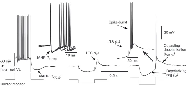
but the kinetics are much slower. If the amplitude of the LTS is sufficient to reach the firing threshold, a burst of high frequency action potentials will be generated. Note that exciting the hyperpolarized cell is not a necessity to trigger an LTS. At the offset of a hyperpolarizing current, it is very likely that the TC neuron will trigger a sponta-neous LTS crowned with Na+ spikes since V
m tends to return to its resting state, which
implies crossing the activation threshold of IT (Fig. 1.8(middle)). The specific range
of action of IT enables TC cells to operate in two different modes (Fig. 1.8(left and
right)). At a depolarized level of Vm, cells are in a tonic-firing mode and a sufficient
stimulus triggers one or several unitary action potentials. Under hyperpolarization, however, TC cells operate in a bursting mode since they have that ability to generate
20 mV 50 ms 10 ms 0.5 s fAHP (IK(Ca)) mAHP (IK(Ca)) LTS (IT) LTS (IT) Spike-burst Depolarizing sag (Ih) -60 mV Intra - cell VL Current monitor Outlasting depolarization (INa(P))
Figure 1.8: Intrinsic electrophysiological properties of thalamocortical neurons. Left, Tonic-firing mode. Middle, Generation of a rebound low-threshold spike at the offset of a hyperpolarizing current pulse. Right, Generation of a low-threshold spike crowned by a burst of action potentials. Note the depolarizing sag induced by the Ihcurrent when a hyperpolarizing current pulse is applied [4]. bursts of high-frequency action potentials. This firing mode suggests the crucial role of IT in thalamocortical oscillations during sleep, i.e. when modulatory (e.g. cholinergic)
inputs are inactivated and cells are hyperpolarized [12–14].
Ih is a mixed Na+ and K+ current that is activated under hyperpolarization of the
membrane (half-activation at Vm =-75 mV) and that is almost completely deactivated
at Vm =-60 mV [35]. As a consequence, when a TC cell is hyperpolarized from Vrest, Ih
is activated and produces a slow depolarization of the membrane. We refer to this slow apparent voltage change in time as the “depolarizing sag” (Fig. 1.8(right)). Since this depolarization may cross the activation threshold of IT, it may contribute indirectly to
the generation of an LTS by activating T-channels. Note also that despite its Na+/K+
nature, it has been demonstrated that Ih has a Ca2+ dependence [36]. This Ca2+
dependence would induce a shift in its activation curve and increase the conductance of the channels underlying this current.
1.1.4
Thalamocortical oscillations
The thalamocortical system has a tendency to oscillate, and to different frequencies depending on the state of vigilance (reviewed in [4]). The various oscillations include the slow (<1 Hz), the delta (1-4 Hz), the spindle (7-15 Hz), the beta (15-30 Hz) and
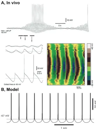
the gamma (30-80 Hz) oscillations, as well as ripples (>100 Hz). Experimental studies have demonstrated the existence of the delta oscillation (1-4 Hz) during slow wave sleep. This activity can be induced independently in both thalamic and cortical structures. An enhancement of the neocortical delta activity has been observed in neocortical slabs, i.e. in a small and isolated part of cortex, and after the surgical removal of the thalamus [37,38]. Thalamic delta oscillations can be intrinsically generated in TC neurons during sleep by an interplay between IT and Ih [35,39–41]. A long-lasting hyperpolarization
of the membrane simultaneously deinactivates IT and activates Ih. The depolarizing
sag recruits IT by opening the activation gates of T-channels before the closing of the
inactivation gates. It results in a burst of action potentials. The inactivation and the deactivation of IT and Ih, respectively, at the depolarized level of Vm induced by the
burst results in a hyperpolarization of the membrane so a new cycle can start (Fig. 1.9). However, the disappearance of synchrony between TC neurons at those frequencies in decorticated cats [42] indicates a minor role of the thalamic delta activity on cortical delta oscillations. In contrast, cortical delta oscillations could bring back the synchrony in TC neurons via the corticothalamic feedback projections.
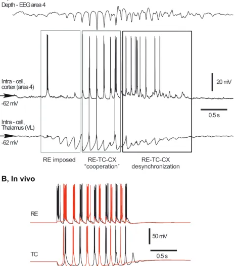
Another type of thalamocortical oscillation is the sleep spindle oscillation (7-14 Hz). It results from both intrinsic and network mechanisms during early stages of sleep or during active phases of the slow sleep oscillation. The presence of thalamic spindle oscillations in decorticated cats points out a thalamic origin of this activity [42–45]. In vivo, in vitro and computational studies showed that such activity can be generated by an interaction between the reticular nucleus and relay nuclei of the thalamus [45–49]. Bursting RE cells induce IPSPs at TC neurons. At the offset of this inhibition, TC neurons generate a rebound burst of action potentials that induces EPSPs at RE cells, thus giving rise to a new cycle of spindle oscillation (Fig. 1.8B). However, it has been shown that TC cells may not fire at every cycle and that RE cells alone can generate these oscillations at their early phase [45,47]. Gap junctions between RE cells [50] is one possible mechanism underlying this independent activity [51]. The second phase results from interactions between RE and TC cells with a contribution of the cortical feedback to these two types of thalamic neuron. The last phase is referred to as the waning phase and is the consequence of a desynchronization of the network [45]. The Ca2+ dependence of I
h may also contribute to the termination of spindle oscillations
by depolarizing TC cells and preventing rebound spikes to occur [52–54]. Given those mechanisms, spindle oscillations display a “waxing-and-waning” fashion (Fig. 1.8A). This 7-14 Hz activity thus lasts 1-3 seconds, but recurs every 5-15 seconds.
1 sec 50 m V -67 mV A, In vivo B, Model
Figure 1.9: Thalamic delta oscillation. A, In vivo recordings from the lateral posterior nucleus of a decorticated cat. Top, Waxing and waning delta activity (2.2 Hz). Bottom, Left, Magnification of three segments of the top panel. LTSs vary in amplitude and do not trigger a burst at every cycles. Bottom, Right, Topographical plot of the delta activity indicates a stable frequency regardless of the amplitude of LTSs. B, A model of a single TC neuron shows that the delta oscillation can be generated intrinsically [4].
20mV 0.5s Depth- EEGarea4 Intra- cell, cortex(area4) -62mV Intra- cell, Thalamus (VL) -62mV 50mV 0.5s RE TC RE imposed RE-TC-CX
“cooperation” desynchronizationRE-TC-CX
A, In vivo
B, In vivo
Figure 1.10: Spindle activity. A, In vivo recordings of cortical (area 4) and TC (ventral lateral nucleus) neurons of a cat showing the three phases of a spindle sequence. B, Computational model of two RE and two TC neurons showing intrathalamic spindle oscillations [4].
1.2
Modeling biophysical processes
1.2.1
The cable theory
The approach taken in the present study is exclusively a modeling one. This is an usual choice since electrophysiological recordings can rarely be carried out at dendrites or practically never be carried out at thin distal dendrites (∼ 0.5-1 µm in diameter). Modeling biological mechanisms implies a transposition of a physiological description into physical and mathematical terms by making a reasonable number of assumptions and simplifications. Because neurons are electrically excitable cells, their transposition into a mathematical formulation comes naturally from the electrostatic theory. In the present subsection is introduced the cable theory, in order to obtain the cable equation, an equation well-known by scientists in the field of computational neuroscience. Some important axioms obtained from simple considerations, but that are crucial for an intuitive understanding of the voltage propagation in neurons are finally discussed. This model has been widely described in scientific literature and it has been largely used for both single cell and network modeling studies (see references [55,56]).
The phospholipid bilayer that composes the plasma membrane is very thin (30-50 ˚
A), so charges that are on one side of the bilayer may attract or repulse charges on the other side and vice versa via electrostatic forces. As a result charges accumulate at the membrane and a capacitance Cm is established across it. Cm is defined by capacitance
per area, typically in µF/cm2. Furthermore, as mentioned in section 1.1.1, the plasma
membrane is not completely impermeable and different ions can move from one side to the other via leakage conductances or more complex types of channels. Different finite values of resistance or non-zero conductance can be assigned to the different types of channels. A constant resistance times units of area is assigned to the leak current and is referred to as the passive membrane resistance Rm, usually expressed in
Ω·cm2. We may also refer simply to this quantity as the membrane resistance, since
active properties are more conveniently described by conductances. Those variable conductances for active channels will be introduced later. The cytoplasm that fills the intracellular space also presents an axial resistance to the charges flowing in dendrites. However, at a given point in a branch, the axial resistance perceived is much lower than the membrane resistance, so charges preferentially move toward the cell body during forward propagation instead of flowing across the membrane. To describe this resistive effect of the intracellular medium, the axial resistivity Ra is commonly used
and is generally expressed in Ω·cm. If we consider a dendritic branch or a segment of a dendritic branch as a cable of length l and constant diameter D, the total cytoplasmic
A im(x, t) Extracellular medium Permeable membrane Intracellular medium P1 P2 x B Vm(x - ∆x, t) Vm(x, t) Vm(x + ∆x, t) ia(x - ∆x, t) ia(x, t) πD∆xCm πD∆x Rm πD2 4Ra∆x Vrest
Figure 1.11: Cable theory. A, Schematic cable. B, Infinitesimal equivalent circuit.
resistance ra associated to this cable is given by
ra =
4Ral
πD2. (1.5)
The resistance of a dendritic cable to the axial current thus decreases as the cable increases in diameter.
Weak electrical gradients in a homogeneous extracellular space are assumed. It implies a constant potential and an infinite conductance for the extracellular medium [5]. Since we are interested in the difference in potential Vm across the membrane, we set
Vext = 0. Note that since the voltage spread is more important along the axis of
a dendritic branch than in its transverse directions [57], both the radial (ρ) and the azimuthal (θ) coordinates in the intracellular medium are neglected. The initial three spatial dimensions problem thus becomes a one spatial dimension problem, i.e. we set Vm(ρ, θ, x, t)=Vm(x, t).
We consider a simple cable with constant geometry and passive properties Cm, Rm
and Ra. The axis of this cable is along the x axis (Fig. 1.11A). By taking an infinitesimal
segment of length ∆x and building its equivalent electrical circuit (Fig. 1.11B), we can extract the spatiotemporal flow of charges. This small RC circuit is composed of a capacitance in parallel to a resistor in order to reproduce the effect of a permeable thin
plasma membrane on the membrane current. The resistor is in series with a battery establishing the reversal potential Vrest. The whole circuit connects to ground outside
the membrane, since the extracellular medium is assumed to be homogeneous and to have an infinite conductance. This circuit is connected to two neighboring small RC circuits via axial resistors mimicking the impact of the cytoplasm on the current in the intracellular medium. According to Eq. (1.5), the total axial resistance associated to a segment of length ∆x and diameter D is 4Ra∆x/πD2. Similarly, the total membrane
resistance and the total membrane conductance are respectively given by Rm/πD∆x
and πD∆xCm. Consider the figure1.11. Vm(x, t) is the membrane potential at point P1
at time t and Vm(x + ∆x, t) is the membrane potential at P2 at time t. The difference
between those voltages is given by Ohm’s law:
∆Vm(x, t)≡ Vm(x + ∆x, t)− Vm(x, t) = −
4Ra∆x
πD2 ia(x, t), (1.6)
where ia(x, t) is the axial current flowing in the intracellular segment of length ∆x,
from point P1 to P2. In the limit ∆x→ 0 we obtain ∂Vm
∂x (x, t) =− 4Ra
πD2ia(x, t). (1.7)
We define im(x, t) as the current flowing across the membrane from P1. A part of
that current flows in the capacitance and another part flows in the resistance of the membrane circuit. We can express im as follows:
im(x, t) = Vm(x, t)− Vrest Rm/πD∆x + πD∆xCm ∂Vm ∂t (x, t). (1.8)
In the absence of active properties, the membrane potential Vrest equals the reversal
potential for the leak current Eleak. Applying Kirchhoff’s current law at point P1 gives
ia(x− ∆x, t) − ia(x, t)− im(x, t) = 0. (1.9)
Since ia(x− ∆x, t) − ia(x, t) = ia(x, t)− ia(x + ∆x, t), Eq. (1.9) can be rewritten in the
following way:
im(x, t) = ia(x, t)− ia(x + ∆x, t). (1.10)
Substituting this expression for im(x, t) in Eq. (1.8) and taking the limit ∆x → 0, we
obtain −∂i∂xa(x, t) = πD Rm (Vm(x, t)− Vrest) + πDCm ∂Vm ∂t (x, t). (1.11) Taking the spatial derivative of Eq. (1.7) and reorganizing it gives
∂ia ∂x(x, t) = − πD2 4Ra ∂2V m ∂x2 (x, t). (1.12)
The substitution of the right-hand side of this last expression into the left-hand side of Eq. (1.11) gives D 4 Rm Ra ∂2V m ∂x2 (x, t) = Vm(x, t)− Vrest+ RmCm ∂Vm ∂t (x, t). (1.13) This partial differential equation (PDE) is a form of the linear cable equation.
Two quantities called the time and length constants can be defined. They are respectively expressed as
τm = RmCm, (1.14)
in units of time, and
λ = # D 4 Rm Ra $1/2 , (1.15)
in units of length. For simplicity, we define the electrotonic potential V as the deviation from the resting potential, i.e. V = Vm− Vrest. Eq. (1.13) can thus be reexpressed as
λ2∂
2V
∂x2(x, t) = V (x, t) + τm
∂V
∂t (x, t). (1.16)
For steady state conditions, i.e. for ∂V /∂t = 0, Eq. (1.16) reduces to an ordinary differential equation (ODE) and its general solution is
V (x) = A1ex/λ+ A2e−x/λ (1.17)
or
V (x) = B1cosh(x/λ) + B2sinh(x/λ). (1.18)
Two boundary conditions are needed to identify constants A1 and A2. Suppose a
semi-infinite cable. The finite end corresponds to x = 0 and is voltage-clamped at V = V0.
The voltage where x→ ∞ implies that V tends to zero when approaching infinity. The unique solution to Eq. (1.17) is thus
V (x) = V0e−x/λ. (1.19)
This expression brings a physical meaning to the length constant. In a semi-infinite cable, λ is the distance over which a steady state voltage is reduced to 1/e) 0.368 times its value at x = 0 or anywhere along the cable. A semi-infinite cable might appear as an impossible condition to fulfill. However, this description of an electrotonic attenuation of the voltage that provides λ applies very well to branches of more than 4λ in length. It can thus be used to treat long-lasting responses in long dendrites.
An equivalent interpretation of the time constant can also be obtained. If we con-sider a cable clamped to V = V0 over all its length, the decay in potential at the offset
of the voltage-clamp will be described by τm. Taking ∂2V /∂x2 = 0 in Eq. (1.16) and
solving the resulting first order differential equation with V = V0 at t = 0, we obtain
V (t) = V0exp[−t/τm]. At the offset of the voltage-clamp, the electrotonic potential
will therefore decay to 0.368V0 after a time t = τm. However, the definition Eq. (1.14)
stands when the voltage mainly decays via a current flow across the membrane. It hardly applies for thin distal dendrites of neurons, where voltage transients rise and decay quickly in distance and time. Even for large sections, like the soma and its near perisomatic region, which are close to isopotentiality, τm does not faithfully describe
the time course of typical responses. This fact previously led to a misevaluation of the time constant in cat motoneurons (see a description of the problem by Rall [58]). Furthermore, it was shown that for fast excitatory synaptic currents, the time course of EPSPs is independent of Rm and thus Eq. (1.14) is certainly not accurate [59]. On
the other hand, one can safely say that anywhere in a cell, the time constant is always smaller or equal to the value provided by Eq. (1.14).
Consider now a finite cable of length l instead of an infinite cable, but that still has the extremity x = 0 clamped to V = V0. If the other extremity at x = l is a sealed end,
the new boundary condition for this extremity is dV /dx = 0 since the voltage spread or the current flow stops at that impermeable end. Using Eq. (1.18) for simplicity, the unique solution in such condition can be expressed as
V (x) = V0
#
cosh(l/λ) cosh(x/λ)− sinh(l/λ) sinh(x/λ) cosh(l/λ)
$
(1.20)
or, using the propriety of hyperbolic functions cosh(a−b) = cosh(a) cosh(b)−sinh(a) sinh(b),
V (x) = V0cosh % l− x λ & cosh(l/λ) . (1.21)
Another special case of a finite cable l is the “open end” condition. The extremity at x = 0 is still clamped at V = V0, while the open extremity at x = l will be assigned
an electrotonic potential V = 0. Since V = Vm− Vrest, we say that the cable is clamped
at its resting potential at x = l. Using a similar approach as for the sealed end, the unique solution can be obtained:
V (x) = V0sinh % l− x λ & cosh(l/λ) . (1.22)
Different voltage spreads for different boundary conditions are shown in figure 1.12. The voltage spread within the cable is largely reduced at shorter distances for cables with an open end than for cables with a sealed end, due to a shunting effect at the open
!"# !"$ !"% !"& !"' !"( !") !"* !"+ ! !"' +"! *"! ,-, ! +"! ! x-! g f e a b c d
Figure 1.12: Voltage spread in cables for different boundary conditions. Curve a corresponds to a semi-infinite cable. Curves b, c and d correspond to the “open end” condition for different cable lengths. There is a shunting effect of the voltage spread due to the open end. Curves e, f and g correspond to the “sealed end” condition. The resistance along the cable is higher than for an open end. As a consequence, the current flow toward the end is weaker and the voltage is higher. For small cable lengths, the membrane tends to become isopotential along the cable. The curve a for a semi-infinite cable is the limit between the “open” and “sealed end” cases. Modified from [5].
end and a reduced resistance along the cable. The case of a semi-infinite cable is at the limit between those two cases.
It is clear from previous results that different responses might be obtained at different positions in a cable or in a neuron depending on boundary conditions. It would also be the case for a transient current instead of a constant current. The response obtained from a current injection may be highly variable at the site of stimulation given different sets of geometrical parameters. Of major interest in this study is the amplitude of the response. An important quantity is the input resistance, which can be measured experimentally at the soma by taking the ratio of the steady voltage to the steady current Iinj applied by an electrode. It is an easy measure to carry out and it provides
an idea of the degree of excitability of a cell. The higher is the input resistance, the higher is the response to an applied current. For a semi-infinite cable, the input resistance Rinat the extremity x = 0 is noted R∞in the literature and can be expressed
as
R∞= (RmRa)1/2
πD3/2
2 . (1.23)
In that case the electrotonic voltage at x = 0 would be
V (x = 0) = R∞Iinj. (1.24)
(1.23) that the input resistance is higher for both higher membrane and axial resistances. For a finite cable of length l in the “open end” condition, Rin < R∞ at x = 0, while
Rin > R∞ for the same cable in the “sealed end” condition. Note also that R∞ is
higher for a finite cable of length l than for a cable of length 2l. From this simple fact, one could expect a cell with extensive dendritic trees to trigger smaller responses at their cell body than a more compact cell. This is what Rall predicted when he studied the voltage spread in branched dendrites [5]. At tested conditions, he even found that the dendritic input resistance Rdend at the connecting point between the soma and
a primary branch reaches the value obtained for an infinite cable when dendrites get sufficiently extensive. Rdend depended only on the first few branching orders and did
not change much whether higher orders were included or not in the model. On the other hand, this statement does not apply for events arising at distal branches since they are electrically isolated. Note also that since Rdend decreases when the amount of
branching in trees increases, the current flow from the soma to dendrites is enhanced for extensive dendrites and smaller and rapidly decaying somatic responses are to be expected. Furthermore, Rin is typically a measure of excitability under the application
of a steady current and one could question the reliability of these facts for a highly transient response, as for an AMPA-receptor-mediated EPSP.
What happens for transient responses? Softky previously obtained an elegant ex-pression from the cable theory describing, after making a few assumptions, the ampli-tude of an EPSP evoked by a fast current input [59]:
Vpeak ≈ 1.5 R1/2a Ipeak (πD)3/2C1/2 m ' tpeak. (1.25)
In this expression, Ipeak is the amplitude of the current applied and tpeak is the time
taken to reach its peak from the onset of the current. In contrast to what provide Eqs. (1.23) and (1.24) for a steady voltage, the amplitude of a fast EPSP given by Eq. (1.25) does not depend on the membrane resistance Rm, but is dependent on the
capacitance. This is an important result. It predicts that the amplitude of an EPSP will grow considerably as the diameter of the targeted branch decreases, but also that it will depend on the membrane capacitance, which would not be really the case for a steady voltage. However, Eq. (1.25) is limited by the fact that the amplitude of an EPSP should depend on the driving potential. The depolarization induced by an EPSP stops to increase when its amplitude gets closer to the reversal potential Esyn of
the synaptic current (∼0 mV, typically). This effect is not taken into account in Eq. (1.25). Note that high in amplitude transient responses are largely attenuated during their propagation to soma, and much more than for the spreading of steady voltage. The reason is that the axial resistance and the membrane capacitance are organized in a distributed low-pass filter. For the same reason, one can expect a fast EPSP to get broadened during its propagation to soma [60–63].
A
B
50 µm
Figure 1.13: Compartmental modeling. A, Three-dimensional reconstructed dendrite. B, Compart-mental model corresponding to the dendrite shown in A.
1.2.2
The compartmental model
In the previous subsection we found solutions of the cable equation for a steady state voltage in different simple conditions. Since the current delivered at a synapse is highly transient, we would like to calculate the response induced at the postsynaptic mem-brane for a transient current. However, evaluating Vm and the propagation of
poten-tials in highly complex arborizations increases rapidly in difficulty. Including nonlinear membrane properties such as intrinsic currents and ionic pumps makes an analytical approach impossible to achieve and makes numerical calculations long to carry out. The best strategy to adopt to solve those problems is the compartmental modeling, a method first developed by Rall [64].
To obtain the cable equation (1.13), we used infinitesimal RC circuits. In fact, one can spatially discretize a complete neuron into a given number of equivalents circuits connected by resistors mimicking the effect of the cytoplasm on the intracellular current
flow. The neuron is thus “compartmentalized” in multiple isopotential segments (Fig.
1.13). A compartment must be small enough so that spatial differences in Vm within
the compartment can be neglected. In the limit of an infinite number of compartments, the solution of the system would approach the exact solution for a continuous cable. However, a relatively low number of segments is needed to reduce the numerical error to a more than acceptable level. Compartments do not need to have all the same size, and the equivalent passive properties cm, rm and ra can be determined easily. By
integrating Cm (µF/cm2) and the membrane leakage conductance gleak(S/cm2) over the
surface area, the total membrane capacitance cm and the total membrane resistance rm
can be calculated. Similarly, the axial resistance ra connecting to the previous and
the next compartments is calculated by taking the integral of Ra (Ω·cm) over the first
extremity to the middle of the segment and over the middle to the last extremity. In the compartmental model, the spatial derivatives of the cable equation (1.13) can be removed. Instead of solving iteratively a continuous PDE for each compartment with proper boundary conditions, we solve a system of coupled ODEs.
Adding various currents to an initially passive model is an easy task in a com-partmental formalism. Consider a single compartment as shown in figure 1.14. Each synaptic or active intrinsic current j can be inserted via an additional parallel conduc-tance gj in series with a battery Ej that fixes the reversal potential of the new current.
Note that gleak = 1/Rm by convention. However, gj is usually not constant and depends
specifically on time t and on Vm. This is why it is represented as a variable conductance
in figure 1.14. The total membrane current can be expressed as im = Cm dVm dt (t) + gleak(Vm− Eleak) + ( j gj(Vm− Ej) (1.26) or, at equilibrium, Cm dVm dt (t) =−gleak(Vm− Eleak)− ( j gj(Vm− Ej). (1.27)
Note also that each current in Eqs (1.26) and (1.27) is in fact a density of current per unit of area, since Cm and the different conductances are respectively in units of
capacitance and conductance per units of area. However, Vm is the absolute membrane
potential.
Compartments need to be connected together. Suppose that ˆimk is the total current
flowing across the membrane of total capacitance cm at the compartment k. By
Kirch-hoff’s current law, ˆimk equals the axial current flowing out of the compartment k− 1
toward k minus the current flowing out of k toward the compartment k + 1:
g
jE
leakg
leakE
jC
mFigure 1.14: General form of a single compartment.
where ˆiak−1,k and ˆiak,k+1 denote the axial currents. This can be reexpressed as
cmk dVm dt (t) + ( j ij = Vk−1− Vk rak−1,k − Vk− Vk+1 rak,k+1 , (1.29)
where rak−1,k and rak,k+1 are the total axial resistances between adjacent compartments.
At bifurcation points, the current flow in daughter branches is taken into account by adding another two terms at the right-hand side of Eq. (1.29) with appropriate indexes. Both daughter branches have the same k− 1 compartment.
If we consider a morphologically complex cell model with N compartments, we end up with a system of N differential equations to solve. It can be written in a matrix formulation:
˙)V = A)V +)b, (1.30)
where ˙)V is a N components column vector containing the time derivatives and )V is a column vector of unknown membrane potentials. A is a N× N matrix containing the coefficients of V1, V2, ..., VN−1 and VN and )b is a column vector containing products
of conductances with their corresponding reversal potential values. Note that A is a sparse matrix, i.e. it mainly contains zeros since one dendritic compartment is gener-ally not connected to more than 2 or 3 neighboring compartments. For a sufficiently fine spatial discretization, the multicompartment model provides good solutions with efficient calculations since the second-order spatial derivatives have been removed from our differential equations.
1.2.3
Modeling active membrane properties of thalamocortical
cells
The existence of active and specific channels was demonstrated by Hodgkin and Huxley in the early 50s. Using voltage-clamp experiments in a squid giant axon, they were able to describe the mechanisms underlying the generation of action potentials. The prolific pair of scientists then established an elegant mathematical formalism for the description of channels kinetics [65]. An intrinsic or a synaptic current j can be modeled using an ohmic relation:
ij = gj(Vm− Ej), (1.31)
where gj and Ej are respectively the conductance and the reversal potential for the
current j. However, gj is usually not a constant factor in Eq. (1.31) and may depend
on time t, on the membrane potential Vm or on other variables. Eq. (1.31) can be
reexpressed in the following way:
ij = gjmMhN(Vm− Ej), (1.32)
where gj is the peak conductance, typically in S/cm2 for intrinsic currents, and m and
h are respectively the activation and inactivation variables and are generally functions of t and Vm. The m variable conceptually represents the ratio of open activation gates,
while h is the ratio of open inactivation gates. Both m and h thus have a value between 0 and 1 and can also be thought of as the probability of finding a gate in its “open” state. The values of M and N are determined from the fitting to experimental recordings. They represent more or less the number of ions of type j needed to open the gate or the number of gates. The functions of m and h are obtained empirically from real electrophysiological recordings in order to reproduce the intrinsic activity of real cells. The passage from an open to a closed state of gates or from a closed to an open state is described by rate equations:
dm
dt = αm(1− m) − βmm (1.33)
dh
dt = αh(1− h) − βhh, (1.34)
where the α and β constants are called rate constants and are functions of Vm, but not
t. By setting Eqs. (1.33) and (1.34) equal to zero, we obtain the steady state values of rate equations: m∞ = αm αm+ βm (1.35) h∞ = αh αh+ βh . (1.36)
Expressions (1.35) and (1.36) describe the voltage dependence of the activation and inactivation processes and can be determined by fitting experimental data. It provides the range of action of a given current in terms of Vm. The remaining information to
obtain is the time dependence of those processes. Time constants can be determined from voltage-clamp experiments. A time constant can be defined for each type of gate:
τm = 1 αm+ βm (1.37) τh = 1 αh+ βh . (1.38)
Rate constants can then be evaluated from experimental data of m∞, h∞, τm and τh,
and a function for rate constants can be constructed. The solutions for the activation and inactivation variables are
m = m∞− (m∞− m0) exp(−t/τm) (1.39)
h = h∞− (h∞− h0) exp(−t/τh). (1.40)
Again the constants m0 and n0 can be obtained empirically. To model currents, one
can use either time constants with steady state values of m and n as in Eqs. (1.39) and (1.40) or Eqs. (1.33) and (1.34) with proper rate constants.
As for all excitable cells, TC neurons possess Na+ and K+ channels that allow them
to generate action potentials. In all simulations we used a model established in a past study on hippocampal PY neurons [66] and that was later used in several modeling studies on TC cells [49,67,68] or on other types of cells [69,70]. The K+ conductance
is expressed as
gK= gKn4. (1.41)
Those channels do not inactivate and are only described by an activation variable n. The rate constants are given by
αn = 0.032(67− Vm) exp ! 67− Vm 5 " − 1 (1.42) βn= 0.5 exp ! 62− Vm 40 " . (1.43)
Similarly, the Na+ conductance is described by
The rate constants for that transient current are αm = 0.32(65− Vm) exp ! 65− Vm 4 " − 1 (1.45) βm = 0.28(Vm+ 12) exp ! Vm+ 12 5 " − 1 (1.46) αh = 0.128 exp ! 69− Vm 18 " (1.47) βh = 4 1 + exp ! 92− Vm 5 ". (1.48)
As mentioned in section 1.1.3, the low-threshold calcium (IT) and the
hyperpolarization-activated cation (Ih) currents are crucial for thalamocortical oscillations during sleep.
In some simulations we used one or both of these currents. The model of IT was
described in a previous study [71] and is based on voltage-clamp data [72]. The kinet-ics of activation and inactivation were later updated [73]. Typically, intracellular and extracellular Ca2+ concentrations are respectively of the order of 0.1 µM and 1 mM,
which is low compared to K+, Na+ and Cl− concentrations (∼ 10-100 mM). The respective
Ca2+ concentrations inside and outside the cell are also highly unbalanced. This imbalance
causes the outward current to be nearly absent since Ca2+ ions hardly move against their
concentration gradient, and thus a reversal potential cannot be deduced from usual consid-erations. The current-voltage relationship for an open channel is nonlinear and Ohm’s law
cannot be used. To describe Ca2+ currents another form of the GHK equation called the
Goldman-Hodgkin-Katz constant-field equation is required. It is dependent on Vmand on the
extracellular ([Ca2+]
ext) and intracellular ([Ca2+]in) calcium concentrations. It is denoted as
G(Vm, [Ca2+]ext, [Ca2+]in) and is expressed as follows: G(Vm, [Ca2+]ext, [Ca2+]in) =
4F2Vm RT
[Ca2+]in− [Ca2+]extexp(−2F Vm/RT )
1− exp(−2F Vm/RT )
. (1.49)
IT is formulated as
IT = PCam2hG(Vm, [Ca2+]ext, [Ca2+]in), (1.50)
where PCa is the maximum permeability of T-channels, typically in cm/s. Activation and
inactivation parameters were obtained from experimental data:
m∞= 1 1 + exp ! −Vm+ 59 6.2 " (1.51) h∞= 1 1 + exp ! Vm+ 83 4 " (1.52)