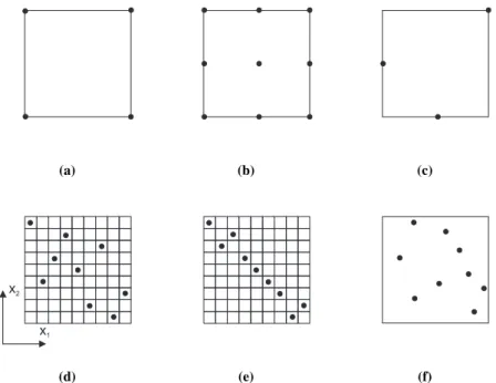
Sensitivity analysis by design of experiments

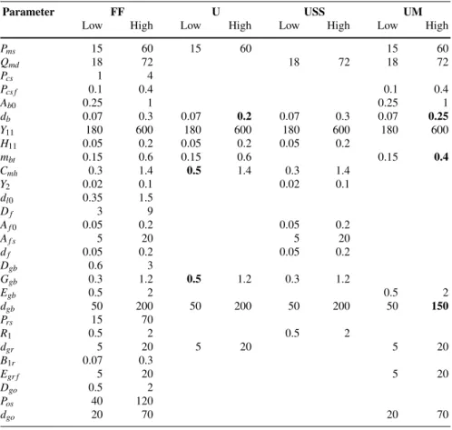
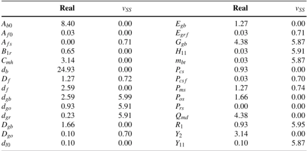
In this study, we have used a global sensitivity analysis method for studying the simulation of fluid pressure and solid velocity full waveform responses in a configuration

Gaillard, Two parameters wronskian representation of solutions of nonlinear Schr¨odinger equation, eight Peregrine breather and multi-rogue waves,

H. ORDER PARAMETER IN THE GLASS TRANSITION OF VITREOUS S-Ge.. It Was found that a side peak at 440 cm is skronger for the slowly quenched glass than for the rapidly quenched

After the internal and external functional analysis is done in ACSP, the user enters the functional parameters in ORASSE Knowledge, because it will be this software, which will

(1998), that the service level is a direct trade off between various cost factors (typically holding vs. cost of stock out). Other would argue that it is determined by

amplitude modes in the biaxial phase mix the components of biaxiality and birefringence of the order parameter, the critical (quasi-biaxial) mode presenting

2014 We present results concerning sample dependence of not only the modulation wave vector, but also of the amplitude of the order parameter describing the N

In this Appendix, we briefly review the theory of the de SQUID in so far as it concems the effects of trie intrinsic phase shift in YBCO-Pb SQUIDS. We wiii assume that in zero