Influence of Complex Environments on LiDAR-Based
Robot Navigation
Mémoire Sébastien Michaud Maîtrise en informatique Maître ès sciences (M.Sc.) Québec, Canada © Sébastien Michaud, 2016Résumé
La navigation sécuritaire et efficace des robots mobiles repose grandement sur l’utilisation des cap-teurs embarqués. L’un des capcap-teurs qui est de plus en plus utilisé pour cette tâche est le Light Detection And Ranging(LiDAR). Bien que les recherches récentes montrent une amélioration des performances de navigation basée sur les LiDARs, faire face à des environnements non structurés complexes ou des conditions météorologiques difficiles reste problématique. Dans ce mémoire, nous présentons une analyse de l’influence de telles conditions sur la navigation basée sur les LiDARs. Notre première contribution est d’évaluer comment les LiDARs sont affectés par les flocons de neige durant les tem-pêtes de neige. Pour ce faire, nous créons un nouvel ensemble de données en faisant l’acquisition de données durant six précipitations de neige. Une analyse statistique de ces ensembles de données, nous caractérisons la sensibilité de chaque capteur et montrons que les mesures de capteurs peuvent être modélisées de manière probabilistique. Nous montrons aussi que les précipitations de neige ont peu d’influence au-delà de 10 m. Notre seconde contribution est d’évaluer l’impact de structures tridi-mensionnelles complexes présentes en forêt sur les performances d’un algorithme de reconnaissance d’endroits. Nous avons acquis des données dans un environnement extérieur structuré et en forêt, ce qui permet d’évaluer l’influence de ces derniers sur les performances de reconnaissance d’endroits. Notre hypothèse est que, plus deux balayages laser sont proches l’un de l’autre, plus la croyance que ceux-ci proviennent du même endroit sera élevée, mais modulé par le niveau de complexité de l’en-vironnement. Nos expériences confirment que la forêt, avec ses réseaux de branches compliqués et son feuillage, produit plus de données aberrantes et induit une chute plus rapide des performances de reconnaissance en fonction de la distance. Notre conclusion finale est que, les environnements com-plexes étudiés influencent négativement les performances de navigation basée sur les LiDARs, ce qui devrait être considéré pour développer des algorithmes de navigation robustes.
Abstract
To ensure safe and efficient navigation, mobile robots heavily rely on their ability to use on-board sensors. One such sensor, increasingly used for robot navigation, is the Light Detection And Ranging (LiDAR). Although recent research showed improvement in LiDAR-based navigation, dealing with complex unstructured environments or difficult weather conditions remains problematic. In this thesis, we present an analysis of the influence of such challenging conditions on LiDAR-based navigation. Our first contribution is to evaluate how LiDARs are affected by snowflakes during snowstorms. To this end, we create a novel dataset by acquiring data during six snowfalls using four sensors simulta-neously. Based on statistical analysis of this dataset, we characterized the sensitivity of each device and showed that sensor measurements can be modelled in a probabilistic manner. We also showed that falling snow has little impact beyond a range of 10 m. Our second contribution is to evaluate the impact of complex of three-dimensional structures, present in forests, on the performance of a LiDAR-based place recognition algorithm. We acquired data in structured outdoor environment and in forest, which allowed evaluating the impact of the environment on the place recognition perfor-mance. Our hypothesis was that the closer two scans are acquired from each other, the higher the belief that the scans originate from the same place will be, but modulated by the level of complexity of the environments. Our experiments confirmed that forests, with their intricate network of branches and foliage, produce more outliers and induce recognition performance to decrease more quickly with distance when compared with structured outdoor environment. Our conclusion is that falling snow conditions and forest environments negatively impact LiDAR-based navigation performance, which should be considered to develop robust navigation algorithms.
Contents
Résumé iii
Abstract v
Contents vi
List of Tables vii
List of Figures ix Acknowledgements xiii Introduction 1 1 Literature Review 5 1.1 Introduction . . . 5 1.2 Snowfall Conditions . . . 5
1.3 Feature-Based Place Recognition and Forest Environments . . . 7
2 Snowfall Influence on LiDAR Data 11 2.1 Introduction . . . 11
2.2 Basics of LiDARs . . . 12
2.3 Data Acquisition . . . 16
2.4 Temporal Analysis . . . 19
2.5 Distribution of Snowflake Echoes as a Function of Range . . . 23
2.6 Discussion and Conclusion . . . 26
3 Forest Influence on LiDAR-Based Place Recognition 27 3.1 Introduction . . . 27
3.2 Data Acquisition . . . 28
3.3 Place Recognition Algorithm . . . 35
3.4 Results. . . 46
3.5 Conclusion . . . 52
Conclusion 55
Bibliography 59
List of Tables
1.1 Examples of popular descriptors and keypoints detectors for images and 3D data. . . 7
2.1 Overview of characteristics specific to each LiDAR. . . 16
2.2 Overview of our snow dataset. . . 18
2.3 Details of measurement selection for the analysis. . . 19
2.4 Overall average snowflake echoes for the complete 02-19 dataset, per sensor. . . 22
3.1 List of devices available on the Husky A200 and their use in our experiments. . . 28
3.2 Details about the point clouds created with our two LiDARs. . . 33
3.3 Datasets acquired for place recognition analysis.. . . 33
3.4 The set of NARF parameters used for the BoW pre-ordering step and the candidate transformations scoring step. . . 42
3.5 A summary of the different scenarios for scoring corresponding pixels of the range images. . . 45
List of Figures
2.1 Example of a LiDAR device and a simplified representation of the laser trajectory. . . 12
2.2 Representation of LiDAR beams in different conditions along with the resulting
wave-forms. . . 14
2.3 Point cloud representation of a LiDAR acquisition and examples of erroneous data
regions. . . 15
2.4 The experimental setup. . . 17
2.5 View from the camera. . . 18
2.6 Four overlaid consecutive scans for the LMS200 sensor, and the first echo scans for
the Hokuyo sensor. . . 20
2.7 Temporal evolution of the percentage of echoes coming from the falling snow within
5 m of the sensors during the 6 most intense snowfall episodes. . . 22
2.8 Cartoon representation of the interaction between the probability of detecting a snowflake and the diminution of snowflakes due to the shielding effect of the building. . . 24
2.9 Histograms of echoes in falling snow during important snowfall days, as a function of
distance reported by the sensor. . . 25
3.1 Our robotic platform (Husky A200) and the devices used for data acquisition. . . 29
3.2 Partial aerial view of the Laval University campus including the two approximate paths
followed by the robot for data acquisition. . . 31
3.3 Images from the UGV camera during the acquisition of the two datasets. . . 32
3.4 Examples of point clouds from our datasets viewed from different perspectives. . . . 34
3.5 Examples of range images from the two datasets. . . 37
3.6 Example of a partial range image and the corresponding point cloud with an example
of edge caused by an object border.. . . 38
3.7 Illustration of a NARF descriptor calculated on a range image patch. . . 39
3.8 Examples of NARF keypoints found for two different scans with examples of
corre-spondences. . . 41
3.9 Path adjusted using ICP for our three datasets. . . 48
Acronyms
2D
Two Dimensional. 2,5,7,12,17,30,46
3D
Three Dimensional.vii,2,7,8,12,13,15,17,30,32,35,36,40–42,44
BoW
Bag of Words.vii,8,40–42,44,53
FN False Negative.49 FOV Field Of View.32,33,52 FP False Positive.49–53,57 GPS
Global Positioning System.1,28,30
GUI
Graphical User Interface.28
ICP
Iterative Closest Point.ix,46–48,53
IMU
LiDAR
Light Detection And Ranging. vii, ix, 2,3, 5,6,8,11–17, 19,23,26–30,33,36, 41,44,49,
51–53,55–57
NDT
Normal Distribution Transform.8
PTU
Pan-Tilt Unit. 12,15,28–30,52
RGB
Red, Green, Blue colour.2,17,18
RGB-D
Red, Green, Blue plus Depth. 7
ROS
Robot Operating System.17,30
SLAM
Simultaneous Localization And Mapping.5,8,27,49,52,56
SSH Secure Shell. 28 TN True Negative.49 TP True Positive.49 UDP
User Datagram Protocol. 32
UGV
Unmanned Ground Vehicle. ix,5,28,32
Acknowledgements
Firstly, I would like to express my sincere gratitude to my advisors Prof. Philippe Giguère and Prof. Jean-François Lalonde, for the continuous support during my Master studies. They seamlessly pro-vided funding and research equipment, they assisted me during the writing, but most of all, they shared their precious knowledge and time to help me reach my goals.
A very special thanks goes out to François Pomerleau, a Postdoctoral Fellow who taught me a lot about the world of research and helped me learn the essential tools for applied robotics. He always answered my numerous questions patiently and provided me with useful tips for my work, even after leaving our research lab.
I would like to thank my fellow lab mates for the help they gave me on multiple projects, the stimu-lating discussions we had and the fun time we shared during social activities.
Introduction
Modern robotics has experienced tremendous growth since its inception during the Industrial Revo-lution. Whether it is to assist humans in their work, to automate some tasks or to perform dangerous tasks, robots are emerging in a wide variety of applications. Recent technology such as the self-driving car project from Google and the BigDog quadruped robot from Boston Dynamics are feats of engi-neering that show how robots have evolved from being able to operate in controlled environments to performing complex tasks in a challenging or unpredictable situations.
One of the key elements that allowed for such progress is the ability of the robot to adapt to changing environments. This is especially true for mobile robotics, where not only the surrounding environment can change, but the robot itself can move and must therefore be able to locate itself. This capability highly depends on algorithms that convert the raw sensor inputs into a convenient representation or abstraction of the environment. This concept is known as artificial perception.
A wide range of sensors are available to assist robots navigation. It is possible, for instance, to estimate the relative movements of the robot using wheel encoders. Unfortunately, when the ground friction coefficient is variable or the load-bearing surface is very uneven, pose estimation relying solely on this sensor is highly unreliable. Similarly, Inertial Measurements Units (IMU) are composed of accelerometers and gyroscopes that can be used to infer changes in position. Although these sensors can be very precise over short distances, they accumulate errors over time, which inevitably leads to a drift on the pose estimation.
The natural solution to this problem is to use sensors capable of providing absolute positioning. Ar-guably the most popular sensor providing such information is the Global Positioning System (GPS). However, there are inherent problems with this sensor as well. GPS requires receiving the signal of at least three satellites at all time. These signals can be blocked by building, terrain, dense foliage or other structures, thus causing important positioning errors or possibly no positioning at all.
Alternatively, a global map of landmarks can be used by the robot to locate itself. These landmarks are distinctive features acquired using sensors that react to external stimuli of the robot environment (i.e. exteroceptive sensors). Visual markers acquired with cameras, sounds signatures obtained with microphones or singular structures detected with sonars are examples of such features. In addition to solving localization and mapping problems, the use of such features make it possible to perform many
other navigation tasks. For instance, it is possible to classify ground type to predict traversability or detect obstacles to compute path planning.
The most widely used sensors for such task is the conventional Red, Green, Blue colour (RGB) cam-era. In addition to its generally low price, cameras provide valuable appearance information about the scene in which the robot operates. This information can be processed, for instance, to analyze geometric elements of the scene or identify objects in it. Despite these obvious advantages, the im-ages obtained by the cameras are produced by a projection and it is difficult or impossible to retrieve information regarding the three-dimensional structure of the scene. Furthermore, the quality of acqui-sitions depends greatly on the lighting conditions of the environment. The processing of these images for real-time navigation requires powerful hardware, which is not always available on the robot. The Light Detection And Ranging (LiDAR) is another sensor that provides valuable data about the scene. It uses a laser to measure distances at different angles from the sensor centre. Most LiDARs provide Two Dimensional (2D) set of points, but some are able to directly produce Three Dimensional (3D)data, called point clouds. LiDARs are generally more expensive than cameras, but the geometrical information obtained therewith is often complementary to the appearance information provided by the cameras. For instance, a LiDAR will faithfully report the flat structure of a white wall, while the lack of visual features will make it impossible for the camera to infer such information. On the other hand, a camera would be able to locate itself using the rich appearance information of a poster on a wall, but the geometrical information of the wall retrieved by the LiDAR is of little help for the localization task. Another important difference between those sensors is that the LiDAR is an active sensor that can be used day and night and which is mostly unaffected by lighting conditions, while the camera is a passive sensor for which the compensation for changes in lighting conditions is among the most challenging problems.
In Chapter1 we will review existing literature about robot navigation. Because cameras were used in the field before LiDARs and because those sensors are somehow similar, techniques used with cameras inspired those for LiDARs. For this reason, there will be references related to cameras, but LiDARs proved to be an excellent choice for robot navigation and will be the sensors of interest of this document. As we will see, existing works for LiDAR mainly deal with simpler situations such as structured indoor or semi-structured city environments. We will therefore focus our attention on more challenging environments such as falling snow conditions or highly unstructured outdoor environments. More precisely, we are interested in the impact of those complex environments on the resulting data and the task to be achieved.
Subsequently, in Chapter2, we will briefly present the basics of how LiDARs operate and how readings are theoretically affected when scanning small structures or dynamic objects. These conditions are likely to be found in many complex environments where the robot might need to navigate. Therefore, we are interested in quantifying the impact such small structures and dynamic objects on the sensor readings. For that matter, we placed four different LiDARs so as to acquire data during falling snow
conditions. Using our experimental setup, we are able to evaluate the influence of snowflakes of various sizes and falling at different rates on the sensors measurements.
Chapter 3 provides a higher level analysis of the influence of the environment on a navigation al-gorithm. In this case, we chose a state-of-the-art LiDAR-based place recognition algorithm and we compared the results obtained in different environments. We created our own dataset in conditions similar to the one presented in the original article and acquired another dataset in forested area. Be-cause forests are composed of multiple small structures such as branches and leaves, we considered the latter dataset more challenging, and found that the radius within which it is possible to recognize places reliably is lower in such environments.
Chapter 1
Literature Review
1.1
Introduction
Mobile robotics literature contains a wide variety of LiDAR-based solutions to navigation problems. This includes using 2D for indoor Simultaneous Localization And Mapping (SLAM) [Grisetti et al.,
2007,Kohlbrecher et al.,2011], geolocation in forest [Hussein et al.,2015] or detection of traversable grass-like vegetation using laser remission [Wurm et al., 2009]. As it is the case for this thesis, some studies focus their efforts on finding solutions for challenging conditions (or environments). It should be noted that there is no clear definition of what constitutes challenging conditions, as it varies between sensors. A good understanding of the LiDAR functioning [Amann et al., 2001] therefore helps understand how it applies to this sensor (see Section2.2). The Marulan Data Sets [Peynot et al.,
2010] contains good examples of such conditions, including natural outdoor environments and area with presence of smoke, dust and rain.
In this thesis, we are interested in the influence of such difficult situations, either due to complex unstructured environments or challenging weather conditions, on LiDAR-based robot navigation. In Section1.2, we will discuss research related to navigation in snowfall conditions, which is the linked to Chapter2. Subsequently, Section1.3will present papers related to feature-based place recognition and navigation in forest environments, which are more closely related to Chapter3.
1.2
Snowfall Conditions
Snowfall conditions are challenging as snowflakes cause occlusion or interference with the laser beam. Because of their small size and dynamic nature, they tend to produce a signal similar to random noise in sensors acquisitions. While it is often possible to avoid navigating in these conditions, some robots will inevitably face this situation in order to perform the tasks for which they were designed.
For instance, Moorehead et al.[1999] aimed at developing a robot to search and classify meteorites in Antartica. In their experiments, the Unmanned Ground Vehicle (UGV) droves autonomously for
10.3 km in different weather and terrain conditions. The navigation was based on stereo camera im-ages and single line LiDAR scans. In this article, the authors explain that the snow-covered surfaces did not provide a lot of visual cues, which made stereo cameras unreliable. For this reason, the robot took advantage of the LiDAR, mainly for obstacle avoidance, but often as single sensor. In return, the authors stated that part of the experiments “was performed during heavy snow which made the laser useless”, and therefore used alternative solutions. As we will see in Chapter 2, new LiDAR technologies help reduce the impact of small particles on the readings.
Another example of robots which need to handle all-weather conditions are those deployed on the battlefield.Yamauchi[2010] uses ultra-wideband radar, stereo camera and LiDAR data for navigation. According to the author, “[LiDAR] and stereo vision provide greater accuracy and resolution in clear weather but has difficulty with precipitation and obscurants”. The ultra-wideband radar has the ability to see through small particles such as snow, rain and fog and is therefore complementary to other sensors used. The final system achieve good results by using traditional sensor fusion, as well as a selective use of the sensors, which are activated or deactivated depending on the conditions.
Sumi et al. [2013], for their part, aimed at evaluating sensors for personal care robots in natural lighting and falling snow conditions. For that matter, they built two simulators that reproduced those conditions and used three types of sensor: an active stereo sensor (Microsoft Kinect), a LiDAR (Mesa SR4000) and a passive stereo sensor (PGR Bumblebee2). This approach is interesting since it allowed to control various parameters that may affect the sensor readings. However, the physical properties of simulated snowflakes can be different from that of real snowflakes, leading to inaccurate results for real applications. By contrast, as we used natural events to estimate the impact of snow flakes on LiDARmeasurements, we were not able to control the environment parameters.
The work by Barnum et al.[2010] is probably the most similar to our work presented in Chapter2, but applied to video rather than LiDARs data. They explain that rain and snow are dynamic process, which causes spatial and temporal fluctuations in videos. Although the spatio-temporal changes appear to be chaotic, they were able to predict the overall effect of these conditions on the video, in frequency space. This modelling of the effect of weather conditions on videos improved the noise filtering for features extraction, when compared to previous pixel-based or patch-based methods.
Finally,Servomaa et al.[2002] have installed a set of sensors for snowfall observation. The system was composed of a radar and a LiDAR that recorded the atmospheric profile up to 6000 m and another radar along with two balances to record snowfall at ground level. Although the installation was fixed and the LiDAR was used only to evaluate transition in cloud conditions, they proposed techniques to estimate snowfall characteristics. Although not specifically mentioned in their paper, these techniques may advantageously be used to adapt the behaviour of the robot depending on weather conditions.
1.3
Feature-Based Place Recognition and Forest Environments
As we will see in more details in Chapter3, place recognition is a useful tool for mobile robot naviga-tion. A robot can determine whether he is in previously visited place or not by comparing its current sensor acquisition with those acquired earlier. Since the relevant information density in the raw sensor data is low, data is usually converted into a representation that better capture the key information. This process is known as features extraction and consist in identifying points of interest from the sensor data (e.g. image), called feature keypoints, and create a descriptor for each keypoint. A descriptor is a vector containing values which should represent the area surrounding the keypoint robustly, even under small disturbance such as different lighting conditions or change of viewpoint.
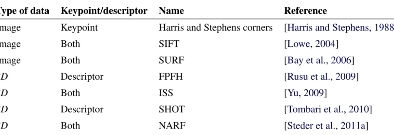
The popularity of using features representation can be attributed to the field of computer vision, es-pecially with the introduction of SIFT [Lowe,2004] and SURF [Bay et al.,2006]. This concept has since been applied to 3D data. Table1.1present some popular 2D and 3D features.
Although the choice of features can influence the performance of place recognition, we will not ad-dress this issue directly in this thesis. Instead, we analyze the impact of some environments on the overall place recognition performance. For those further interested in this topic, a number of articles that present comparative evaluation of different features are available in the literature. For instance,
Filipe and Alexandre[2014] present an evaluation of 3D keypoint detectors, more precisely for Red, Green, Blue plus Depth (RGB-D)objects. In this paper, they focus on the invariance of keypoints detectors to rotations, scales and translation. Similarly, Boyer et al.[2011] propose a benchmark to estimate how different algorithms perform for retrieving keypoints and descriptors when subject to different geometric transformations.
Type of data Keypoint/descriptor Name Reference
Image Keypoint Harris and Stephens corners [Harris and Stephens,1988]
Image Both SIFT [Lowe,2004]
Image Both SURF [Bay et al.,2006]
3D Descriptor FPFH [Rusu et al.,2009]
3D Both ISS [Yu,2009]
3D Descriptor SHOT [Tombari et al.,2010]
3D Both NARF [Steder et al.,2011a]
Table 1.1 – Examples of popular descriptors and keypoints detectors for images and 3D data. Some 2Dkeypoints have been adapted for 3D such as Harris and Stephens and SIFT.
Several techniques have been proposed to solve the place recognition problem, but most approaches use cameras as primary sensor [Torralba et al.,2003,Ulrich and Nourbakhsh,2000]. The most note-worthy example is probably the work ofCummins and Newman[2008], commonly referred as FAB-MAP. They used a probabilistic framework to recognize previously seen places and identify new
places. The algorithm was able to recognize the redundant visual information that did not signifi-cantly help to distinguish places, which was used to reduce the probability of such examples to be labeled as originating from the same place. They reach recall of 48 % at 100 % precision for a dataset of 1.9 km. The authors also proposed an enhanced version of the algorithm [Cummins and Newman,
2011] in which they focus on scaleability primarily using the concept of inverted index. They are able to reach 48 % recall at 100 % precision on a 70 km dataset. As we will see in Chapter3, place recog-nition is often used to detect loop closures for SLAM. In this scenario, the presence of false positives is often catastrophic, which is why they present the results for a precision of 100 %.
By contrast, existing place recognition algorithms based on 3D LiDAR data only are quite limited. To the best of our knowledge,Magnusson et al.[2009] are the first to address this problem. They used Normal Distribution Transform (NDT)to create feature histograms based on surface orientation and smoothness to represent each scan. They also aligned scans with respect to dominant surface orien-tation to achieve roorien-tation invariance. Finally, they used expecorien-tation maximization to automatically determine the threshold that separated corresponding from non-corresponding scans. They achieved recall rates between 22.9 % and 69.6 % with false positive rates below 1.17 %, for three different datasets. More recently, Röhling et al. [2015] proposed a similar approach for solving the place recognition problem based on 3D lidar data. The authors indicated that they used simpler histograms and a different distance metric to achieve similar results toMagnusson et al.[2009]. The main contri-bution of their algorithm is that it is simpler to implement and less computationally demanding. The two previously mentioned algorithms used global descriptors (i.e. a single descriptor for each scan), which is often faster to process but less robust to local disturbances than approaches based on local features (i.e. a set of feature keypoints and associate descriptors for each scan). For our experiments in Chapter3, we will use the algorithm proposed bySteder et al.[2011b], which is itself an extension of their previous work in [Steder et al.,2010]. The algorithm, that will be presented in more details in Section3.3, use a mixture of Bag of Words (BoW) and features matching to recognize places.
To our knowledge, none of the previously discussed algorithms have been tested in forest environ-ments or have been developed for specific conditions, but were rather proposed as generic solutions. When the environment in which the robot will operate is known in advance, algorithms can be de-veloped or fine-tuned using this prior knowledge to potentially improve performance. For instance, one could intuitively assume that in forest, tree trunks are more reliable features than foliage. Lat-ulippe et al.[2013] proposed to use machine learning to automatically identify and filter local point cloud features in natural environments to be robust for scans alignment purpose. In their paper, they indeed concluded that features produced in foliage regions are not reliable. Other examples of prior knowledge used for LiDAR-based navigation in forest include [Lalonde et al.,2006], which present a technique for segmenting data in three classes and [Mcdaniel et al.,2012], which present a technique for segmenting ground and trees in forest. These segmented regions of data can be used to identify navigable area or be used as features for multiple tasks.
An example algorithm using this type of feature, specific to the forest, is presented in Song et al.
[2012a]. They proposed a localization solution using the largest group of approximately parallel tree trunks as features to align successive scans along five dimensions (ignoring the translation relative to the gravity vector). Similarly, Miettinen et al.[2007] created a global map of trees in the form of a graph. In this graph, nodes represented tree trunks and edges represented the distance between those trunks. This representation was then used for localization and mapping, by using best matched sub graphs.
Chapter 2
Snowfall Influence on LiDAR Data
2.1
Introduction
An internal representation of the environment is essential for robots to perform the various tasks for which they are designed. If such representation is not provided beforehand, which is often the case, it will be created using sensors available on the robot. Unfortunately, each sensor acquires a specific type of data in a limited measurement interval. In addition, either because of the sensor itself or because of the acquisition environment, the data obtained are always noisy. While this can be of little influence for some simple problems, ignoring these problems can cause serious misunderstanding of the scene and lead to the failure of the tasks, potentially causing damage to the robot or injuring humans. As we will see in this chapter, LiDARs enable us to assess the three-dimensional structure the environment, but they are especially noisy when measuring dynamic objects, small structures or object edges. Forested area and falling snow conditions are good examples of such challenging environments for LiDARs. Characterizing how LiDARs will react in those conditions will allow us to develop more robust and versatile algorithms.
In this chapter, we will first introduce the basics of LiDARs operations (in section 2.2) to better understand why they are affected by small structures. We will follow up with our main contribution, that is to provide a characterization of the behaviour of four well-known LiDARs in snowy conditions. Through an extensive empirical study performed on a novel dataset captured under varying degrees of snowfall, we evaluate how much these LiDARs are sensitive—or not—to falling snow. We show that recent advances in sensor designs have increased their robustness even to significant snowfall. Section2.3 describe how data acquisition was performed, section2.4present a temporal analysis of the data and section2.5describe the distribution of snowflake echoes as a function of range before we conclude in section2.6.
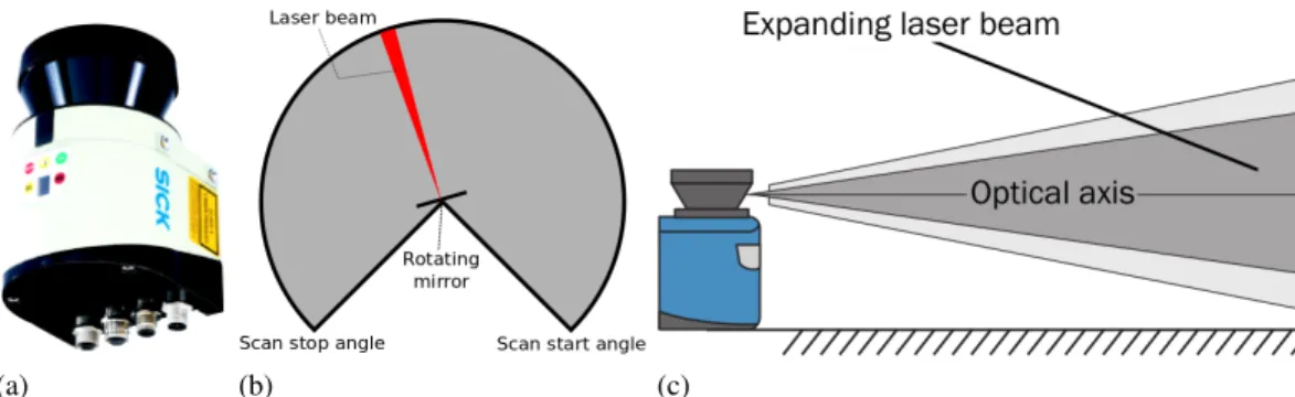
(a) (b) (c)
Figure 2.1 – Example of a LiDAR device and a simplified representation of the laser trajectory. (a)
The SICK LMS151 LiDAR. The truncated cone of the upper part is the place from where the laser is projected and is made of a material allowing the laser to pass through unaffected. (b)A simplified representation of how the internal rotating mirror change the scanning angle of the laser. (c)A side view of the laser beam going out of the LiDAR (figure modified from [SICK,a]).
2.2
Basics of LiDARs
LiDARis a technology based on laser time of flight to measure distances.Amann et al.[2001] present the physical details as well as the pros and cons of three time of flight techniques commonly used in LiDARs, namely the pulsed, phase-shift and frequency modulated continuous wave. Although the LiDARs we will use for our research are all based on time of flight, the underlying technique is not specified by the manufacturers. In the context of our research, we focus more on higher level concepts that could cause sensor readings to be erroneous for modelling environments or objects.
LiDARs generally build 2D data points using an internal rotating mirror (see Figure2.1b). It is possible to create a 3D point cloud by moving the sensor with an external tool (e.g. a Pan-Tilt Unit (PTU) or the robot itself) and merging scans. There are some sensors, such as the Velodyne HDL-32E, that directly provide this 3D information. Given that the points are acquired sequentially, dynamic objects may be distorted in the final representation. Figure2.3bdepicts a point cloud created using the 2D SICK LMS151 mounted on a PTU.
Beams emitted by a LiDAR have a given width and angle at source. This causes the beam two-dimensional pattern on the target to grow with distance. Once the light hits the target, it bounces back to the sensor which will extract the range information from it. Obviously, when the target material is highly absorbent or reflective, the light might not reach the sensor, therefore causing missing data points. Otherwise, the sensor will receive the signal which may be represented by a curve of light intensity as function of time. Smooth lambertian surfaces will produce a unimodal distribution from which it is easy to calculate the target range, but multimodal waveforms caused by partially transparent material, fog, dust, small objects and edges lead to an ambiguous interpretation. Figure2.2depicts laser beams hitting different targets along with the resulting waveforms. While some LiDARs provide full waveform, they generally only output a single or few echoes and the inference method differs between sensors (e.g., using the first or last waveform peak, using the mean). For this reason, it is
important to determine whether the sensor is well suited to the needs.
In order to visualize more easily the data obtained with a LiDAR, they are typically represented by a point cloud. Building such point cloud only consists in converting each distance inferred from a laser return into a point in the 3D space. Figure2.3shows an example of a scene(a)and the corresponding point cloud representation(b). There are also highlighted regions of the point cloud where examples of reading errors caused by the environment surrounding the robot can be seen.
In this document, we focus our attention on the impact of small structures such as the branch presented in Figure2.3bregion D. More specifically, the present chapter deals with the impact of falling snow on the raw data of LiDARs. In the next section (Section2.3), we will explain how we gathered data for this analysis.
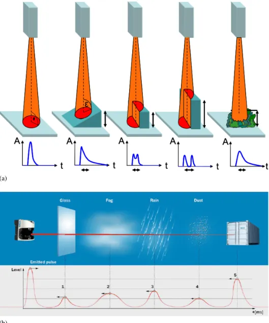
(a)
(b)
Figure 2.2 – Representation of LiDAR beams in different conditions along with the resulting wave-forms. (a)Different unimodal and multimodal distributions resulting from different target structures. FromJutzi and Stilla[2006].(b)The multimodal waveform resulting from a laser beam going through multiple translucent material. From the SICK LMS500-21000 Lite website [SICK,b].
(a)
(b)
Figure 2.3 – A picture of a scene (a) and a diagonal view of the point cloud(b) resulting from the acquisition by the SICK LMS151 LiDAR mounted on a PTU. The sensor position is represented by A. Region B shows missing points caused by absorbent material (a black box not visible in the picture). Region C shows noisy points caused by the edge of an object while region D shows a particularly bad 3Drepresentation of a fine structure (tree branch).
2.3
Data Acquisition
In this section, we report on the relevant characteristics of the four sensors used in our dataset. We then describe the physical configuration of our test setup, then outline the weather conditions pertaining to each of the six collected snowfalls. Finally, we describe how the information from the LiDARs was preprocessed before analysis.
2.3.1 Sensors
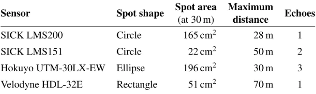
Data acquisition was performed with the following four LiDARs: the SICK LMS200, SICK LMS151, Hokuyo UTM-30LX-EW, and the Velodyne HDL-32E. Relevant sensor information is provided in Table2.1, but the reader is referred to the manufacturers’ documentation for additional information1. The first element that gives a qualitative overview of the sensor performance is the maximum acquisi-tion distance. This value depends on several factors, such as lighting condiacquisi-tions and target remission. This value is provided directly for the HDL-32E and UTM-30LX-EW, but based on a target remission greater than 75 % for the LMS200 and LMS151. Another element to consider is the shape and area covered by the beam, which influences the probability of hitting a snowflake as well as the proportion of area it covers. A final significant element which changes from one sensor to the other is the num-ber of echoes returned. The Hokuyo sensor can return up to three echoes, which means that it could locate two snowflakes before the beam reaches the ground. Regarding the LMS151, two echoes are evaluated by the hardware, but only one is returned. Finally, note that all LiDARs use class 1 laser with a wavelength of 905 nm.
2.3.2 Setup Configuration
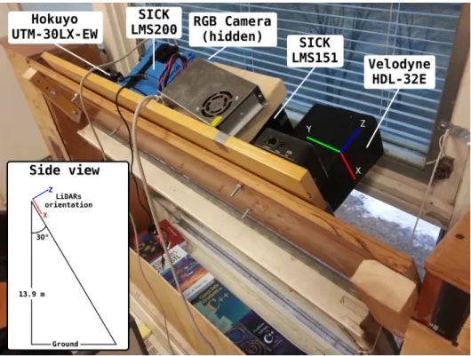
Data acquisition was conducted at Pouliot Hall of Laval University, where sensors were placed close to the inner wall of a window facing N50°E. As shown in Figure2.4, a wooden structure held the sensors side by side at approximately 14 m above the ground. The main scanning plane (i.e. XY plane in the sensor reference frame) formed a 30° angle with respect to the building wall, so as to increase the maximum distance as much as possible without having the laser beams hitting trees or a
1Available here: Velodyne [Velodyne,a], Hokuyo [Hokuyo], LMS151 [SICK,c], LMS200 [SICK,2006]
Sensor Spot shape Spot area
(at 30 m)
Maximum
distance Echoes
SICK LMS200 Circle 165 cm2 28 m 1
SICK LMS151 Circle 22 cm2 50 m 2
Hokuyo UTM-30LX-EW Ellipse 196 cm2 30 m 3
Velodyne HDL-32E Rectangle 51 cm2 70 m 1
Table 2.1 – Overview of characteristics specific to each LiDAR.
Figure 2.4 – The experimental setup. The 3D axis represents the orientation of the sensors and the bottom left panel represent the 2D geometry as seen from the right side of the picture.
pedestrian walkway present near the building. In addition, an RGB camera was placed alongside the LiDARs to provide visual information about the scene. In this configuration, a slight opening of the window allowed to keep the instruments inside while scanning outside. To avoid direct interference between sensors, corrugated plastic layers were placed between them. Figure2.5shows the scene as observed by the RGB camera placed with the sensors.
2.3.3 Dataset Description
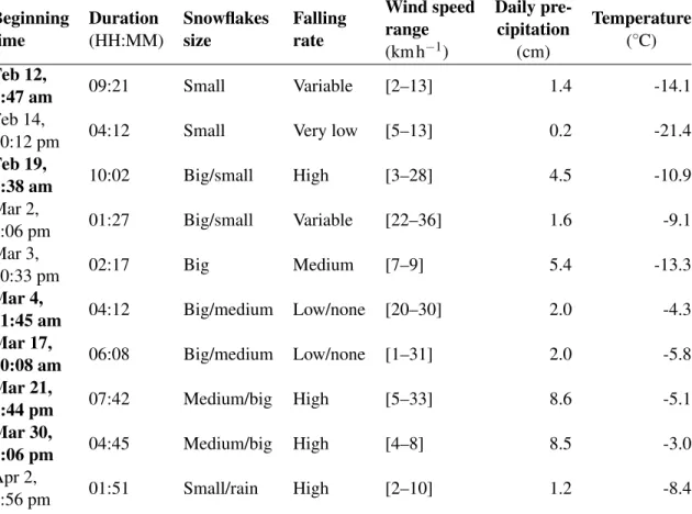
Data acquisition started February 12 and ended on March 2. A total of 10 episodes were collected for a total of more than 50 hours of data. Recordings were made using the Robot Operating System (ROS)[Willow Garage], which provides standardized data types as well as time synchronization. Data was acquired at different times of day and in a wide variety of conditions, covering a wide range of snowflakes size, falling rate and wind speed. Table2.2 provides an overview of our data2. Of these, six are used in the current study, as highlighted in this table.
2.3.4 Pre-Selection of Laser Data
For each sensor, we selected a combination of angles and laser rings (for the Velodyne) or angles (for the others) that had a clear view of the snow-covered ground surface. The actual details for each
2Wind speed, daily precipitation and temperature are reported from Québec City Jean Lesage International Airport at
Figure 2.5 – View from the RGB camera. Beginning time Duration (HH:MM) Snowflakes size Falling rate Wind speed range (km h−1) Daily pre-cipitation (cm) Temperature (◦C) Feb 12, 9:47 am 09:21 Small Variable [2–13] 1.4 -14.1 Feb 14,
10:12 pm 04:12 Small Very low [5–13] 0.2 -21.4
Feb 19, 8:38 am 10:02 Big/small High [3–28] 4.5 -10.9 Mar 2, 1:06 pm 01:27 Big/small Variable [22–36] 1.6 -9.1 Mar 3, 10:33 pm 02:17 Big Medium [7–9] 5.4 -13.3 Mar 4, 11:45 am 04:12 Big/medium Low/none [20–30] 2.0 -4.3 Mar 17, 10:08 am 06:08 Big/medium Low/none [1–31] 2.0 -5.8 Mar 21, 6:44 pm 07:42 Medium/big High [5–33] 8.6 -5.1 Mar 30, 1:06 pm 04:45 Medium/big High [4–8] 8.5 -3.0 Apr 2, 1:56 pm 01:51 Small/rain High [2–10] 1.2 -8.4
Table 2.2 – Overview of our snow dataset. Dates in bold correspond to the six days used in the present study.
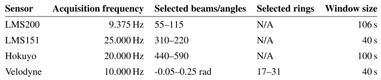
Sensor Acquisition frequency Selected beams/angles Selected rings Window size
LMS200 9.375 Hz 55–115 N/A 106 s
LMS151 25.000 Hz 310–220 N/A 40 s
Hokuyo 20.000 Hz 440–590 N/A 100 s
Velodyne 10.000 Hz -0.05–0.25 rad 17–31 40 s
Table 2.3 – Details of measurement selection for the analysis. The window size is the temporal window used to calculate statistics during the temporal evolution of a snowfall.
sensor are given in Table2.3. The range of the ground in our scans was between x=15 m to x=22 m, depending on the angle. To simplify the analysis, we considered as a snowflake echo any measurement which had a range reading of x < 14.5 m. As will be shown later in sec. 2.5, this approximation is valid as the vast majority of those events happened for x < 10 m.
2.4
Temporal Analysis
In this section, we analyze the temporal behaviour of the four sensors for the duration of six complete snowstorms. In particular, we are interested in seeing how the fraction of echoes in snowflakes evolves over time, for all four sensors. First, we will discuss the highly dynamical nature of snowstorms. This will be exemplified by how consecutive scans can have significant quantitative and spatial differences in the distributions of the snowflakes echoes, which justify the use of averaging windows for our analysis. We will then present the actual temporal evolution of these statistics in the form of graphs for all four sensors, and finally briefly discuss the results for each sensor.
2.4.1 Extraction of Temporal Statistics
Snowstorms are highly dynamic processes, with large variation in snowfall rates over their durations. Moreover, the snow physical characteristics (size, shape or reflectance) might vary significantly during a storm, affected by ambient conditions such as humidity level and temperature. Also, wind gusts might pull snow back up in the air or drive it sideways, affecting its effective fall rate. Consequently, one expects during a snowstorm to see significant short, medium and long-term variations in the fraction of LiDAR echoes corresponding to the falling snow.
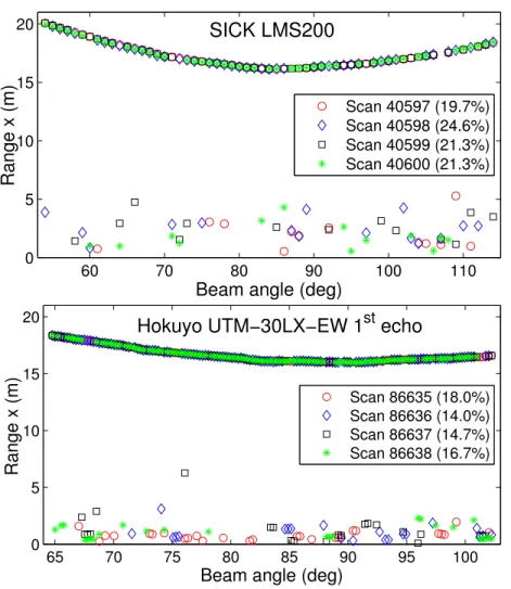
Computing and reporting the temporal statistics for every scan would put too much emphasis on the very short-term statistics. Indeed, the inter-scan variation in the fraction of snowflake echoes can be significant. To better illustrate this point, we have overlaid four consecutive scans in the same plot for the LMS200 and for the first echo returned by the multi-echo Hokuyo sensor in Figure2.6, for an intense snowing episode from the 02-19 dataset (see Table 2.2). In these figures, we can see strong variations in the fraction of snowflake echoes and their spatial distribution, which we believe can be best described as a random process. One can readily see the fluctuation in these fractions as reported
60 70 80 90 100 110 0 5 10 15 20
Beam angle (deg)
Range x (m)
SICK LMS200
Scan 40597 (19.7%) Scan 40598 (24.6%) Scan 40599 (21.3%) Scan 40600 (21.3%) 65 70 75 80 85 90 95 100 0 5 10 15 20Beam angle (deg)
Range x (m)
Hokuyo UTM−30LX−EW 1st echo
Scan 86635 (18.0%) Scan 86636 (14.0%) Scan 86637 (14.7%) Scan 86638 (16.7%)
Figure 2.6 – Four overlaid consecutive scans for the LMS200 sensor (top), and the first echo scans for the Hokuyo sensor (bottom), taken from the 02-19 dataset. Each symbol corresponds to a particular scan. The curved line at the top corresponds to the snow surface on the ground. One can see the rapid variation of the snowflake echoes between scans, and how they are mostly limited to a range x < 5 m. The percentages (in brackets) are the proportion of those echoes in the snowflakes.
in the brackets of the legend in Figure2.6.
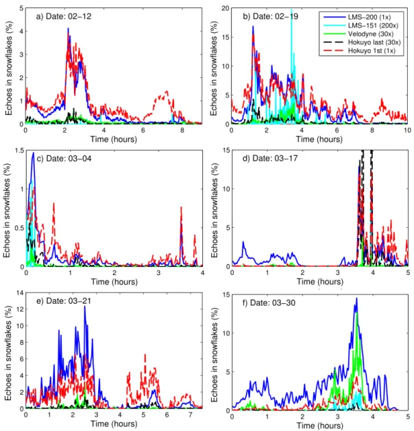
To smooth out these fluctuations, statistics are extracted from a number of consecutive scans contained in a time window of around 1 minute (detailed values in Table2.3). Figure2.7shows this smoothed fraction of snowflake echoes compared to all returned laser measurements as a function of time, for the six snowiest days of our dataset. To allow for better visualization, only the LMS200 and the Hokuyo’s first echo are plotted at their actual scale (1x): Others have been scaled up (from 30x to 200x), with their corresponding scaling factors reported in the legend. As will be shown below, some sensors were much more sensitive than others.
2.4.2 Detailed Analysis, per Sensor
SICK Sensors LMS200 and LMS151
Our first conclusion based on Figure2.7is that the most sensitive device was the older LMS200, first introduced in the mid-2000s. For the most intense snowstorms (Figure 2.7. b) 02-19, d) 03-17, e) 03-21 and f) 03-30), it peaked at around 15% of measurements triggered by the falling snowflakes, for averaging windows of 106 s. As an older-generation device, it probably uses less sophisticated algorithms and sensing, and was not directly targeted for harsh outdoor environments. Indeed, its technical description [SICK,2006] indicates that “Raindrops and snow-flakes are cut out using pixel-oriented evaluation”, but this seems only applicable to obstacle detection (field computation), not the actual measurements. No further details are given. On the other hand, the more recent SICK LMS151 exhibits much less sensitivity to snowflakes: The reduction factor for the fraction of snowflakes echoes is in the order of 200-300, granting this device a much higher immunity in snowstorms. Indeed, the highest peak was around 0.1 % of echoes in snowflakes during the 02-19 dataset. In some sense, this is not surprising considering that the documentation from the manufacturer mentions that this model is targeted for “all-weather conditions” [SICK,a].
Hokuyo UTM-30LX-EW
For this sensor, we resorted to a slightly different approach for comparison, as the device has been designed to return multiple echoes. We thus extracted statistics for the two most relevant cases: for first and last echoes. Statistics for the first echo tell us how sensitive the device is, if one wishes to detect the presence or absence of falling snow. This information could be used, in turn, to adapt the driving strategy of an autonomous vehicle or inform vision algorithms of the presence of particles in the air. On the other hand, using the last echo increases the probability that we will detect obstacles, such as another vehicle or the snow-covered ground. This information would be used for localization and navigation purposes. In the case of the first echo, we observed that the device behaved similarly to the LMS200. Indeed, the Hokuyo first echo (blue line) closely tracks the LMS200 curves (red dashed line) almost everywhere in Figure2.7, with a few exceptions. In the case where we look at the last echo, the sensor behaves like the LMS151, not surprisingly as this sensor does a 2-echoes analysis and filtering. The last echo of the Hokuyo tends to reject the falling snow, but not as well as the LMS151, as it peaked at around 0.5 % in some episodes. Nevertheless, this difference might not be sufficient to impact algorithms relying on laser data. Note that Table2.4shows similar correlations between these three sensors, for the averages taken over the complete 02-19 dataset.
Velodyne HDL-32E
For all purposes, the behaviour of the Velodyne was similar to the last echo of the Hokuyo sensor. This is seen both in the temporal behaviour in Figure2.7and in the average value displayed in Table2.4.
Figure 2.7 – Temporal evolution of the percentage of echoes coming from the falling snow (range x<5 m) during the 6 most intense episodes, for all 4 sensors. The data is smoothed by taking statistics for small-time windows. Except for the LMS200 and Hokuyo first echo, all other sensors statistics have been scaled up (factor in brackets of legend b) for ease of visual comparison. Time is in hours, starting from the beginning of the data capture sequence.
LMS200 Hokuyo first echo Hokuyo last echo LMS151 Velodyne HDL-32E
2.67% 3.55% 0.0113% 0.00178% 0.0100%
Table 2.4 – Overall average snowflake echoes for the complete 02-19 dataset, per sensor. These averages are significantly lower than the instantaneous values displayed in Figure2.7, as snow was not falling at all times during that period.
2.5
Distribution of Snowflake Echoes as a Function of Range
In the previous section, we showed how the expected fraction of snowflake echoes varied temporally during snowstorms. In some sense, it provided for a temporal modelling of the interaction between a snowstorm and a given LiDAR. In this section, we evacuate the temporal aspect and instead focus on how the range x affects the probability for a snowflake to trigger a measurement. To this end, we will use histograms to estimate a probability density function of those events, and show that for the weather conditions and the sensors we tested, there seems to be an upper bound on the range x beyond which falling snowflakes no longer trigger a measurement: In other words, snowflakes become invisible to the sensor past a certain range.
2.5.1 Modelling the Impact of Range on Snowflake Detection
When modelling a range sensor, one has to have an idea of the probability distribution of certain events (e.g. snowflakes) as a function of this range. Over the years, many researchers have proposed probabilistic models for sensors, notably inBurgard et al. [2006]. In the previous section, we have in some sense estimated the probability for a given sensor S that a snowflake would generate an echo Esnowflakegiven the weather conditions W , or PS(Esnowflake|W). In this section, we take a closer
look at which range x such events would be generated, that is PS(Esnowflake|x,W). Having such a
formulation would allow for a more statistically-sound treatment of the information, such as within a Bayesian probabilistic framework. To this effect, we use histograms as approximations to the previous distribution. In Figure2.9, we have plotted these histograms for each of the four sensors. For ease of comparison, they have all been normalized by their total area in the interval 0 < x < 14 m, as the total count varies widely between the sensors. The numbers in brackets in the legend indicate the fraction of echoes in the snowflakes compared to the total number of data points, for a given dataset.
The general shape of these histograms is close to a log-normal distribution, with the exception of the LMS200 for a number of dates (02-12 through 03-17), which seems to follow a sum of two log-normal distributions. We attribute this log-normal shape to the interaction between two different phenomena, illustrated in a cartoon-type model in Figure 2.8. At short ranges x < 3 m, the building acts as a shield and decreases the probability of having a snowflake in the path of the laser. We recognize that this phenomenon would be most likely absent on an autonomous vehicle, thereby increasing the probability of having echoes in snowflakes at close range. However, we believe that this difference is not problematic, as close obstacles would be easily detected from i) the overwhelming number of LiDARechoes on this obstacle ii) other sensing modalities such as vision or radar. Furthermore, if the LiDARis to be mounted on a rooftop, one can safely ignore echoes in the first 2 m, either in software or directly through the sensor itself (via its configuration). The other phenomenon, illustrated as the red dashed line in Figure2.8, is the probability of optical detection of a snowflake by the sensor as a function of the range x. We argue that this shape is due to the rapidly decreasing light intensity of the echoes in snowflakes, as a function of x. Combining these two phenomena yields a log-normal shaped curve (black line in Figure 2.8). Overall, this seems to indicate that a simple probabilistic
0 5 10 15
Range x (m)
Probability of
snowflake detection
Building shielding effet Optical detection Product of both
Figure 2.8 – Cartoon representation of the interaction between the probability of detecting a snowflake (in red) and the diminution of snowflakes due to the shielding effect of the building (in blue). The black line is the product of the two, and bear a close resemblance to the actual histograms extracted from our dataset.
model PS(Esnowflake|x,W)can be derived for these sensors.
2.5.2 Sensor Results
As can be seen from the histograms in Figure2.9, most sensors exhibit the log-normal or sum-of-log-normal distributions discussed above. We note that for certain days, the distributions are shifted to the right (greater range x). In particular, for the 03-21 and the 03-30 distributions, this shift is substantial (on the order of 1 m). We suspect that for these days, the snowflakes were significantly larger, thus allowing for a stronger optical echo and extended range of detection.
For all sensors, we can also conclude that beyond the range x > 10 m, snowflakes are no longer detected, i.e. they become invisible. A small notable exception would be for the Velodyne, for which snowflakes were detected all the way to x=14 m, albeit at a significantly reduced rate. Again, we do not think that this would significantly impair their use in conditions similar to our test setup.
0 2 4 6 8 10 12 14 Distance x (m) Normalized density a) LMS200 02−12 (0.53 %) 02−19 (2.67 %) 03−04 (0.12 %) 03−17 (0.82 %) 03−21 (1.77 %) 03−30 (3.04 %) 0 2 4 6 8 10 12 14 Distance x (m) Normalized density b) Velodyne 02−12 (0.0021 %) 02−19 (0.0100 %) 03−04 (0.0002 %) 03−17 (0.0013 %) 03−21 (0.0023 %) 03−30 (0.0267 %) 0 2 4 6 8 10 12 14 Distance x (m) Normalized density c) LMS151 02−12 (0.00001 %)02−19 (0.00178 %) 03−04 (0.00005 %) 03−17 (0.00013 %) 03−21 (0.0023 %) 03−30 (0.00052 %) 0 2 4 6 8 10 12 14 Distance x (m) Normalized density d) Hokuyo 1st echo 02−12 (0.80 %)02−19 (3.55 %) 03−04 (0.15 %) 03−17 (0.80 %) 03−21 (1.48 %) 03−30 (0.61 %)
Figure 2.9 – Histograms of echoes in falling snow during important snowfall days, as a function of distance x reported by the sensor. Each histogram has been normalized by its area, for ease of compar-ison. The numbers in brackets are the fraction of data points in the complete dataset that correspond to snowflake echoes. Note that for the 03-21 dataset, the LMS151 was not working properly: thus no data is included for that day.
2.6
Discussion and Conclusion
In this chapter, we explored the impact of falling snow on the usability of 4 commonly deployed LiDARs. To this end, we first presented an overview of LiDARs functioning and possible causes of noise in the measurements. As explained, the small size and dynamic nature of snowflakes make snowstorms perfect examples of challenging condition when using LiDARs.
For our experiments, we collected data during 6 snowstorms in the winter of 2015. Upon analysis, we found that the SICK LMS200 was the most sensitive LiDAR, having a peak average rate of up to 15 % of echoes coming from falling snow. Meanwhile, all three others never exceeded 1 %. We also presented a simple probabilistic model to take into account the effect of the range on snowflakes interference. Based on a histogram analysis, we concluded that for our experimental setup, this model can be approximated by a log-normal distribution. Most importantly, our data indicate that the impact of snowflakes on LiDAR beyond a range of 10 m is very limited.
However, a number of questions remains to explore. For example, as the LiDAR beam travels through the falling snow, its intensity will diminish. Since the maximum range of a LiDAR is heavily related to this beam intensity, we expect the maximum range to be affected during snowstorms. In our setup, we have not witnessed this issue, indicating that this effect probably happens beyond our maximum distance of 20 m. Another aspect to be investigated is the relationship between the returned intensities and the surface type (ground or snowflakes). Also, because of the shielding effect of the building, very few snowflakes were present at close range; It might be the case that at closer range, a snowflake might be detected at more than one angle, effectively occluding small targets. Moreover, we have not investigated the impact on the measurement noise for the snowy ground surface in the presence of falling snow.
Chapter 3
Forest Influence on LiDAR-Based Place
Recognition
3.1
Introduction
In order to navigate safely and efficiently in their environments, mobile robots have to be able to solve a multitude of problems. An example of such problems is the ability to determine whether the robot is located in a place it visited before or in a new, unvisited one. Despite the fact that this question seems relatively elementary, solving the so-called place recognition problem is useful for a wide variety of applications. For instance, multiple robots can cooperate to concurrently build a global map (multi-session mapping) using recognized places as connecting points between the different local maps [Howard,2004]. The well-known "kidnapped robot" problem, which consists in determining if the robot has been carried to an arbitrary location, can also be solved using a place recognition algorithm. Because such algorithms do not rely on odometry and allow a robot to locate itself relative to all previously visited places, it is possible to detect this kind of unpredictable change of location. Finally, place recognition algorithms are useful to perform SLAM. The most obvious use is for a topological representation, where the map consists of places and links between them, but it is also essential for loop closure (often referred as the "front-end") when using a metric representation. In the previous chapter, we analyzed the influence of an environment with snowy condition on the LiDARdata. Following the same idea, we are now interested identifying the impact of challenging en-vironments when performing place recognition using LiDAR. More precisely, we want to evaluate how unstructured environments, such as forests, influence navigation algorithms performance. To this end, we chose to use a state-of-the-art LiDAR-based place recognition algorithm developed bySteder et al.
[2011b]. Their algorithm proved to be successful in structured indoor and semi-structured outdoor en-vironments. In our experiments, we produced our own datasets in forests, but also in semi-structured conditions for comparison purposes. Besides the influence of the type of environment, we are also interested in the impact of the sensor used and data associated with it. For this analysis, we used
Device Manufacturer Model Use
Computer – – Data acquisition/synchronization
Gateway Microhard System Inc. VIP2400 Network and Wi-Fi communication Gamepad Logitech F710 Remote control of the robot movements
LiDAR Velodyne HDL-32E Point cloud acquisition
LiDAR SICK LMS151 Point cloud acquisition
PTU FLIR Motion Control Systems D46-17 Rotate the SICK LiDAR
IMU ChRobotics UM6 Odometry
Camera Axis M1013 Visual reference
GPS NovAtel SMART6 Not used
Table 3.1 – List of devices available on the Husky A200 and their use in our experiments. Note that both LiDARs were never mounted at the same time.
two sensors, namely the SICK LMS151 and the Velodyne HDL-32E. The chapter is divided as fol-lows, Section3.2 details where and how the datasets were produced, as well as the resulting data. Thereafter, fundamental concepts related to the place recognition algorithm and the algorithm itself will be presented in Section3.3. Finally, the results of the comparative analysis will be presented in Section3.4before we conclude.
3.2
Data Acquisition
In the following section, we first describe the robotic platform and sensors used to gather our place recognition dataset. We then describe in more details the dataset acquisition procedure and the result-ing data.
3.2.1 Robotic Platform
The Husky A200 is a medium size (990 mm × 670 mm × 390 mm) UGV developed by Clearpath Robotics. It is a rugged robot designed for all terrain conditions and it uses a differential-drive skid steer, allowing easy control and in-place turns. The maximum speed of the vehicle is 1 m s−1 and the maximum payload capability is 75 kg. This robotic platform is well suited for our needs, because it can move in forests and carry the required equipment. Our platform is shown in Figure3.1and details about the available devices are presented in Table3.1.
The on-board computer (2.4 GHz Intel i5-520M) is an essential element of our experiments, as it connects all devices, acts as a control interface for the robot and stores the acquired data. The computer does not provide a Graphical User Interface (GUI), but is connected to the gateway that broadcasts a WiFi network, allowing Secure Shell (SSH) communication. The platform is also equipped with a wireless gamepad, which enables manual control of the movements of the robot. Point clouds
Figure 3.1 – Our robotic platform (Husky A200) and the devices used for data acquisition. The SICK LiDARis not mounted, but instead is shown on the bottom right corner of the figure. Note that the PTUis hidden by a cover and the on-board computer is mostly occluded by the Velodyne LiDAR.
acquisition is possible using either the SICK LMS151 or the Velodyne HDL-32E. The selected sensor is mounted on the PTU, which remains fixed for the Velodyne, but is rotated with the SICK to merge multiple 2D scans into a single 3D point cloud. Section3.2.2gives more details about the resulting point clouds for each sensor.
The sensors described above are essential for our place recognition research, but we also use the wheel encoders along with the IMU for odometry estimation and the camera for visual reference of the dataset. Note that we do not use the GPS, as it is not reliable in forests.
3.2.2 Dataset Description
Data acquisition was performed using ROS, a set of software libraries and tools created to simplify the development of robotics applications. It provides, out of the box, all drivers for the Husky and our sensors. Its data publishing system provides timestamps that allow easy synchronization between sensors. The recording tool (rosbag) was used to create our datasets, with data processing performed a posteriori.
We produced datasets in two different areas of the Laval University campus. An aerial overview of the path followed by the robot at these two locations is presented in Figure3.2.
The first site was chosen for its more structured nature and is located between the Alexandre-Vachon and the Adrien-Pouliot buildings. This environment is mostly open, the terrain is smooth and flat and the site contains man-made objects such as buildings, stairs or tables. Examples of pictures acquired by the robot on this site are presented in Figure3.3aand3.3b. This dataset closely resembles the kind of data on which several place recognition algorithms are typically tested on (e.g. Freiburg Campus 360 degrees 3D scans [Universität Freiburg], Robotic 3D Scan Repository [Nüchter and Lingemann]). The second site, chosen for its unstructured nature, is located in a wooded area, also on the Laval University campus. The dataset path starts on a pedestrian walkway, but after its second turn (of approximately 330°), it continues for around 100 m in rougher terrain. This forested environment presents multiple small structures and significant of occlusions. Figure3.3c and Figure3.3dshow pictures from the robot camera at this location. This dataset will allow us to better understand the in-fluence of a less structured environment on the place recognition algorithm. In particular, the absence of large flat surfaces and corners typical of buildings, as well as the closeness of the space, will be challenging for place recognition algorithms.
To evaluate the impact of the sensor used and data associated with it, we will use the SICK and the Velodyne, for which you can find details in Table3.2.
The SICK is a 2D LiDAR with a scanning angle of 270°, a resolution of 0.5° and an acquisition frequency of 50 Hz. This sensor was placed on the PTU so that the blind spot faced downward. During acquisition, it was rotated around the vertical axis (pan) at a speed of 14.32 ° s−1 for half a turn, while the vehicle was stationary. This procedure allowed the acquisition of 628 2D scans of
(a)
(b) (c)
Figure 3.2 –(a)Partial aerial view of the Laval University campus including the two approximate paths followed by the robot for data acquisition. (b)Zoomed view of the path followed (counterclockwise from tag 1) in a structured environment. The length of this path is approximately 160 m. (c)Zoomed view of the path followed (clockwise from tag 2) to create the unstructured datasets. The length of this path is approximately 275 m. Images source: Google Earth, (2015)
(a) (b)
(c) (d)
Figure 3.3 – Images from the UGV camera during the acquisition of the structured dataset(a) (b)
and the unstructured dataset(c) (d). Note that the images are at an angle for the unstructured dataset, because the camera was not aligned with the robot during acquisition.
540 points, later merged into a single 3D point cloud. To create the dataset using the SICK, the robot was stopped at regular intervals on the established path to acquire scans.
The Velodyne, for its part, directly allows 3D point cloud acquisition by spinning 32 lasers around its vertical axis. These lasers are evenly distributed between −30.67° and 10.67° relative to the hori-zontal plane. According to the Velodyne datasheet [Velodyne,b], the device acquires approximately 700 000 points s−1 and publishes at 10 Hz, therefore creating point clouds of 70 000 points. Note that these point counts are variable as the rotation speed can change slightly and the use of the User Data-gram Protocol (UDP)can lead to some loss of points. Regarding the dataset acquisition, the robot was driven at a constant speed (0.3 m s−1) and performed data acquisition simultaneously. In order to obtain a quantity of scans similar to that produced with the SICK, only one out of 80 scans was used to create the final dataset.
Table3.2summarizes information about the sensors resolution and Field Of View (FOV), while Ta-ble3.3provides a name for later references and additional information about each of our datasets.
Sensor Horizontal resolution Vertical resolution Minimum angle Maximum angle Point counts SICK LMS151 0.57° 0.5° −45.00° 90.00° 339120 Velodyne HDL-32E 0.16° 1.33° −30.68° 10.67° 72000
Table 3.2 – Details about the point clouds created with our two LiDARs. The minimum and maximum angles are given relative to an horizontal plane in the sensor frame of reference and both sensors report 360° around the vertical axis. The point counts represent the maximum number of points in the resulting point cloud.
Dataset name Site Sensor Date NL1 NL2
Structured-SICK Structured SICK LMS151 July 16th, 2015 81 83 Unstructured-SICK Unstructured SICK LMS151 July 14th, 2015 94 92 Unstructured-Velodyne Unstructured Velodyne HDL-32E May 28th, 2015 104 104 Table 3.3 – Datasets acquired for place recognition analysis. We define a name for each dataset in order to facilitate reference thereto in the remainder of this document. NL1 and NL2 represent the
number of scans acquired during the first and second loop respectively.
Examples of point clouds from our datasets are shown in Figure3.4. We observe that the unstructured environment is more congested and objects are closer to the sensor than for the structured environment. In fact, the average distance of points from the sensor in the unstructured environment is 7.61 m compared to 9.23 m for the structured environment. There is also more space without obstacles in the sensor range for the structured dataset. The percentage of points return using the SICK is 82.6 % on average in the unstructured dataset compared to 40.2 % in the structured dataset. These point clouds also illustrate the higher vertical resolution and larger FOV of the SICK compared to the Velodyne. The influence of these factors will be discussed in Section3.4.
(a) (b)
(c) (d)
(e) (f)
Figure 3.4 – Examples of point clouds from our datasets viewed from different perspectives. (a)and
(b)show acquisition from the SICK in the structured environment.(c)and(d)also show point clouds from the SICK, but in the unstructured environment. Finally,(e)and(f)show the result of acquisition from the Velodyne in the unstructured environment. Robot position is represented by a red sphere with a 1 m radius in each picture.
3.3
Place Recognition Algorithm
While there are a number of articles presenting place recognition algorithms using different sensors (e.g. camera [Cummins and Newman,2011], stereo-camera [Cadena et al.,2012]), the literature of such algorithms based solely on 3D data is limited. For our place recognition analysis, we choose to evaluate on our datasets the state-of-the-art algorithm (at the time of the experiments) developed by Steder et al.[2011b] on our datasets. We will first describe some fundamental concepts used for place recognition in Section3.3.1and then we will give an overview of the Steder algorithm itself in Section3.3.2. For the interested reader, the full details of the algorithm are available in [Steder et al.,
2011b].
3.3.1 Fundamental Concepts
The following subsection is an introduction to basic concepts for understanding 3D place recogni-tion algorithms in general. In particular, convenrecogni-tional methods for representing and comparing 3D acquisitions will be presented.
Feature Keypoints and Descriptors
The first step in determining whether or not a place has been visited before, is to convert the sensor data into a format that is more convenient for identification. The generally adopted representation is a vector of real numbers, called a descriptor. This mathematical representation aims at being more compact than the original data while trying to capture significant characteristics from a recognition point of view.
A descriptor can be global, meaning that it tries to capture information about the whole scan, or local, meaning that it does the same but only for a specific subregion of the scan. When using local descriptors, one needs to select the keypoints around which the descriptors will be extracted. These keypoints can be at pre-determined and fixed locations (e.g. division in a simple grid) or selected using more refined algorithms. A common practice for the latter is to choose keypoints in so-called interesting regions which are often defined as regions of high gradient (e.g. edges, corners), as these regions generally contains more information than smooth surfaces. Note that, for simplicity, we might use the term features as a more general term for keypoints and their respective descriptors in the remainder of this document.
The concepts of keypoints and descriptors first originated from the computer vision literature. More recently, they have been adapted for 3D data. Some popular examples of features for both types of data are shown in Table1.1. Note that some algorithms propose solutions for both keypoints detection and descriptors (e.g. SIFT, NARF). However it is not mandatory to use them together as any combination is generally valid. While all features are different, they were all developed with the same goals in mind: