arXiv:1112.0862v1 [astro-ph.SR] 5 Dec 2011
Astronomy & Astrophysicsmanuscript no. zetapup1 c ESO 2011
December 6, 2011
A detailed X-ray investigation of
ζ
Puppis
⋆
I. The dataset and some preliminary results
Ya¨el Naz´e
1,⋆⋆, Carlos Arturo Flores
2, and Gregor Rauw
1 1 GAPHE, D´epartement AGO, Universit´e de Li`ege, All´ee du 6 Aoˆut 17, Bat. B5C, B4000-Li`ege, Belgiume-mail: naze@astro.ulg.ac.be
2 Departamento de Astronomia, Universidad de Guanajuato, Apdo Postal 144, Guanajuato, GTO, Mexico
Preprint online version: December 6, 2011
ABSTRACT
Aims.ζPuppis, one of the closest and brightest massive stars, was the first early-type object observed by the current generation of X-ray observatories. These data provided some surprising results, confirming partly the theoretical predictions while simultaneously unveiling some problematic mismatches with expectations. In this series of papers, we perform a thorough study of ζ Puppis in X-rays, using a decade of XMM-Newton observations.
Methods. ζPuppis was observed 18 times by XMM-Newton, totaling 1Ms in exposure. This provides the highest-quality high-resolution X-ray spectrum of a massive star to date, as well as a perfect dataset for studying X-ray variability in an “archetype” object.
Results.This first paper reports on the data reduction of this unique dataset and provides a few preliminary results. On the one hand, the analysis of EPIC low-resolution spectra shows the star to have a remarkably stable X-ray emission from one observation to the next. On the other hand, the fitting by a wind model of individual line profiles recorded by RGS confirms the wavelength dependence of the line morphology.
Key words.X-rays: stars – Stars: early-type – Stars: individuals: ζ Puppis
1. Introduction
With its very early spectral type (O4Infp, Walborn 1972)
and a distance of only 335 pc (van Leeuwen, 2007;
Ma´ız Apell´aniz et al., 2008), the star Naos, better known as ζ Puppis (or HD 66811), is one of the closest and brightest massive stars. It is therefore one of the most studied objects amongst the O-star population. However, despite the intense work, many open questions remain on its nature.
Indeed, ζ Puppis displays several intriguing properties. First, its visible spectrum shows clear signs of helium overabundance and chemical enrichment by CNO-processed material (e.g. Pauldrach et al. 2001) as well as fast rotation (more than 200km s−1 for v sin(i), Penny 1996; Howarth et al. 1997). Second, it
is a known runaway (e.g. from Hipparcos data, Moffat et al. 1998). These properties have led to speculations on its evo-lutionary status. On the one hand, the chemical enrichment and fast rotation could result from mass and angular mo-mentum exchange through Roche lobe overflow in a binary. ζPuppis could therefore have been the secondary component of such a system, the supernova explosion of its companion having ejected it from its birth place a few millions years ago (van Rensbergen et al., 1996). On the other hand, ζ Puppis dis-plays a similar Hipparcos parallax as stars of the Vela R2 associ-ation1(Schaerer et al., 1997), and dynamical interactions within
⋆ Based on observations collected with XMM-Newton, an ESA
Science Mission with instruments and contributions directly funded by ESA Member States and the USA (NASA).
⋆⋆ Research Associate FRS-FNRS
1 This conclusion was based on the original release of the Hipparcos
catalog, hence the use of the ‘old’ distance of 430 pc in the Schaerer
this association could have led to the ejection of the (single) O-star (van Rensbergen et al., 1996). In this scenario, the chemi-cal enrichment of ζ Puppis would be explained by the intense rotational mixing occurring in the fast-rotating main-sequence progenitor (Meynet & Maeder, 2000). In addition, ζ Puppis dis-plays double-peaked emission lines, suggested to arise in a ro-tating wind (Conti & Leep, 1974; Petrenz & Puls, 1996), and a compression of the wind in the equatorial plane was detected by Harries & Howarth (1996).
Due to its brightness, ζ Puppis was one of the first mas-sive stars observed with high-resolution in X-rays (Kahn et al., 2001; Cassinelli et al., 2001). At first, its X-ray lines appeared to match expectations as they did show the broad, blueward-skewed profiles expected for the wind embedded shock model (Owocki & Cohen, 2001). However, the devil was in the de-tails. When quantitatively fitting the line profiles, Kramer et al. (2003) found a much lower wind attenuation than expected on the basis of the mass-loss rate determined from optical and UV observations (see also Oskinova et al. 2006). They also found that the typical optical depths τ∗, used in the
wind-shock models, seemed independent of wavelength, which can only be explained by invoking porosity (Feldmeier et al., 2003; Oskinova et al., 2006). To improve the fitting of the X-ray line profiles, Leutenegger et al. (2007) included the effect of res-onance scattering: better fits were indeed obtained, without the need of a large reduction in the mass-loss rate, but they also showed that some unexplained discrepancies remain. Re-analyzing the Chandra data of ζ Puppis, Cohen et al. (2010)
ar-et al. paper, but the parallax similarity remains when using the new reduction of Van Leeuwen (and thus the ‘new’ distance of 335 pc).
Ya¨el Naz´e et al.: A detailed X-ray investigation of ζ Puppis
gue in favor of a reduced mass-loss rate, without the need of any porosity as their new derivation of the optical depths implies an increase with wavelength, as expected from the bound-free ab-sorption opacity of the (cool) wind. Except for Leutenegger et al. (2007), all above studies relied on a single 68 ks Chandra obser-vation or a 57 ks XMM-Newton exposure taken in 2000. Both facilities have their advantages: while XMM-Newton globally has a higher sensitivity, Chandra has a lower background, and a higher spectral resolution and sensivity at short wavelengths for its grating spectra. Today, however, much more data are avail-able (see below).
Considering the uncertainties in the line profile results and the lack of new variability studies, we decided to re-investigate ζPuppis using the best dataset available at the present time: 18 XMM-Newton exposures, corresponding to an exposure of 1Ms totaling >700 ks of useful time (i.e. an improvement by an order of magnitude compared to most previous studies). This dataset thus provides the most detailed X-ray view of an O star to date. The results that we obtained will be presented in a series of pa-pers. The first one will present the data, their reduction, and a few first results; the second one will focus on the X-ray varia-tions of ζ Puppis, using EPIC and RGS data; the last one will present a global analysis of the high-resolution X-ray spectrum, using the merged high-resolution data.
This first paper is organized as follows. The dataset and its reduction are presented in Sect. 2, the spectral fits are presented in Sect. 3, the individual line profile fitting in Sect. 4, and the results are summarized and discussed in Sect. 5.
2.
XMM
-Newton observationsIn the past decade of XMM-Newton observations, the star ζPuppis was observed 18 times, mostly for calibration pur-poses. These datasets are excellent for studying the variability of ζ Puppis since (1) the scheduled exposure times were often long (up to ∼60 ks) and (2) the observing dates probe weekly, monthly, and yearly timescales. Unfortunately, many observa-tions were affected by soft proton background flares, resulting in total exposure times reduced by about 30%. Total net expo-sure times for EPIC-MOS, EPIC-pn, and RGS amount to 579 ks, 477 ks, and 751 ks. A summary of the observations is given in Table 1. The successive columns provide the dataset ID (obsID and revolution number); the date at mid-exposure (in the format dd/mm/yy + UT time and JD–2 450 000., calculated using the start/end times of the observations listed in the on-line ’observa-tion lokator’); the mode as well as the scheduled, performed, and effective (i.e. after cleaning flares) exposure time for both EPIC-MOS and EPIC-pn instruments; the scheduled, performed, and effective exposure time for RGS. An empty column indicates a discarded or unavailable dataset (see below). Note that the target was placed off-axis in two observations (5.95′ off-axis in Rev.
0731 and 1.1′off-axis in Rev. 0903).
2.1. EPIC data
The EPIC data were reduced with SAS v10.0.0 using calibration files available on January 1 2011 and following the recommen-dations of the XMM-Newton team2. Different modes (small
win-dow, large winwin-dow, full frame, timing) as well as different filters (thick, medium) and position angles were used for these observa-tions, resulting in a somewhat heterogeneous dataset. To ensure
2 SAS threads, see
http://xmm.esac.esa.int/sas/current/documentation/threads/
the most homogeneous analysis, hence a meaningful comparison between datasets, two decisions were taken. First, a few observa-tions were discarded: those when the instruments were not “on” (aka CAL CLOS ED), those totally affected by flares, those with the source appearing totally or mostly in a CCD gap, those with very short exposure times (<10 ks), those taken in timing mode, and those using a unique combination of mode+filter. This trim-ming process results in a final dataset composed of 9 observa-tions taken with large window + thick filter and 6 observaobserva-tions taken with small window + thick filter for EPIC-MOS; 10 ob-servations taken with small window + thick filter, 5 obob-servations taken with large window + medium filter mode and 4 observa-tions taken with large window + thick filter for EPIC-pn (see Table 1). Second, the extraction regions were chosen to be as constant as possible. A single source region was used for EPIC-MOS, whatever the mode, but two background regions were de-fined, one for each mode since it was not possible to extract the background on the same CCD chip as the source for the small window mode. For EPIC-pn, a single source region was used for all modes, as well as a single background region for the large window mode but four different background regions were nec-essary for the small window mode. Table 2 gives the position and shape of each of these regions.
2.1.1. Pile-up
ζPuppis is rather bright in X-rays, with EPIC count rates of ∼2 cts s−1 (for MOS) and ∼6.5 cts s−1 (for pn with thick filter).
These count rates are at the pile-up limit from the XMM Users’ handbook for the large window modes (i.e. 1.8 and 6 cts s−1for
MOS and pn, respectively) but well below the limits for the small window mode (i.e. 5 and 50 cts s−1 for MOS and pn,
re-spectively). Some pile-up may thus affect our EPIC data taken in the large window mode. To see how severe the pile-up is, we performed several checks. First, we inspected the event files: no event with PAT T ERN=26–29 was found. The pile-up is thus moderate. Second, we run the SAS task epatplot: some small but significant deviation from the “no pile-up” configuration is detected for the large window data, especially those taken with the medium filter.
To get rid of the pile-up, we could extract the data in an an-nulus centered on the source. This would require the anan-nulus to be perfectly centered on the source, especially since the PSF is far from being symmetric. Getting the exact position of ζ Puppis in the datasets is however an impossible task. Indeed, the detec-tion algorithm is also disturbed by pile-up, so that the posidetec-tion found in this way for ζ Puppis is not accurate. For example, the pipeline-processed data from Rev. 1620 yields a position some 2.5” away from the Hipparcos position of ζ Puppis (this sepa-ration is the maximum found in the pipeline-processed data), while a dedicated run of the detection algorithm using only the
PAT T ERN=0 events gives a position that is only 1.2” away. One
would immediately think of using nearby X-ray sources associ-ated with well-known stars - sources which are less bright in X-rays (thus unaffected by pile-up) but still bright enough to get an accurate position in each dataset. However, such nearby sources do not exist in the neighbourhood of ζ Puppis. A perfect cen-troiding of annular regions is thus impossible and using always the Hipparcos position for annular regions may alter the source’s properties, hence the results of the variability study that we wish to perform.
Y a ¨el N az ´e et al .: A d et ai le d X -r ay in v es tig at io n o f ζ P u p p is 0157160901 0542 2002-11-24T20:26:10 2603.352 LW+thick 43.4 43.4 42.9 LW+thick 14.1 14.1 13.2 43.6 43.6 43.0 LW+medium 24.6 24.6 20.9 0157161101 0552 2002-12-15T04:53:31 2623.704 LW+medium 24.2 24.0 11.5 45.6 38.9 26.9 0159360101 0636 2003-05-30T19:28:01 2790.311 LW+thick 66.8 62.7 18.8 SW+thick 42.8 42.7 24.3 72.9 69.2 56.2 0163360201 0731 2003-12-07T02:47:04 2980.616 LW+thick 61.2 52.6 32.4 62.9 53.6 35.8 0159360301 0795 2004-04-12T17:33:58 3108.232 LW+thick 63.9 41.8 19.0 SW+thick 30.2 30.2 17.4 64.1 61.3 21.1 0159360401 0903 2004-11-14T01:57:57 3323.582 LW+thick 21.9 21.9 21.6 SW+thick 29.8 29.8 20.9 77.0 63.0 48.2 0159360501 0980 2005-04-16T14:39:28 3477.111 LW+thick 29.3 29.3 29.0 SW+thick 63.8 63.8 22.1 64.2 64.2 31.0 SW+thick 34.1 27.7 13.4 0159360701 1071 2005-10-15T04:04:52 3658.670 SW+thick 59.6 22.2 15.5 60.0 30.0 27.5 0159360901 1096 2005-12-04T01:14:14 3708.552 SW+thick 59.8 53.5 46.2 SW+thick 59.6 53.3 33.1 60.0 53.5 43.1 0159361101 1164 2006-04-17T21:48:48 3843.409 LW+thick 58.0 42.9 40.1 58.2 52.9 40.5 0414400101 1343 2007-04-09T22:49:29 4200.451 SW+thick 63.7 63.7 47.3 SW+thick 63.5 63.5 34.2 63.9 63.9 48.8 0159361301 1620 2008-10-14T01:15:08 4753.552 SW+thick 66.2 61.2 53.3 SW+thick 66.0 61.0 38.3 66.4 61.5 54.7 0561380101 1814 2009-11-04T06:17:00 5139.762 SW+thick 64.1 64.1 62.1 SW+thick 63.9 63.9 44.7 64.3 64.3 60.5 0561380201 1983 2010-10-07T23:09:52 5477.465 SW+thick 76.7 76.7 74.3 SW+thick 76.5 76.5 53.5 76.9 76.9 65.9
Total exposure time 771.2 679.9 579.2 791.6 734.0 477.0 1066.7 979.7 750.7
Ya¨el Naz´e et al.: A detailed X-ray investigation of ζ Puppis
On the other hand, there is an alternative way in cases of mild pile-up: using only PAT T ERN=0 events. After such a fil-tering, we compared the PAT T ERN=0 spectra extracted in a cir-cular region with the spectra extracted in annular regions (hence free of pile-up) using the usual PAT T ERN=0–12 for MOS and
PAT T ERN=0–4 for pn. This check was done by fitting simple
2-temperatures models on LW+medium data from Rev. 0156, LW+thick data from Rev. 0731 and SW+thick data from Rev. 1814 for EPIC-pn, and on LW+thick data from Rev. 0156 and SW+thick data from Rev. 1814 for EPIC-MOS. The compari-son is excellent for EPIC-MOS data: fluxes and count rates dif-fer by <1% and best-fit spectral parameters are within the errors. The remaining difference can be attributed to the slightly larger noise in the spectra extracted in annuli and from calibration dif-ferences. The comparison is less perfect for EPIC-pn, especially for the data taken with the medium filter: the flux differences reaches 6% in this case, and best-fit spectral parameters are at 2-σ from each other. The pile-up thus still has a small influence on the EPIC-pn data taken in the large window mode, and those data should thus be considered with caution.
2.1.2. The final files
A final check was made on the data from Rev. 1620, which yields the most discrepant (2.5”) position for ζ Puppis, if we trust the pipeline processing. We first derived the position of ζ Puppis from the PAT T ERN=0 data using the SAS task edetectchain, and then extracted the spectra using a circular region centered on that position. We compared these spectra to those extracted on PAT T ERN=0 data using a circular region centered on the Hipparcos position of ζ Puppis. Both sets of spectra appear iden-tical in Xspec: the small centroiding errors have thus no impact on the spectra as long as a circular region is used.
We therefore extracted lightcurves and spectra of ζ Puppis in a circular region centered on the Hipparcos position of the target. We used only the PAT T ERN=0 event files. While this is not necessary for the small window mode, it ensures a homogeneous data reduction. Xspec v12.6.0 was used to fit spectra, and our own software to analyze EPIC lightcurves.
Note that spectra were grouped using the new SAS task
specgroup. It enables to reduce the oversampling, which may
“cause problems during spectral fitting because the spectral bins are then not completely independent” (excerpt from SAS 10.0.0, online documentation). We choose an oversampling factor of 5, ensuring that no spectral bin is narrower than 1/5 of the full width half maximum resolution at the central photon energy of the bin. Note that, while providing more statistically correct data, this process dramatically reduces the number of spectral bins. The data were also grouped to ensure that a minimum signal-to-noise of 3 was reached in each spectral bin of the background-corrected spectra.
2.2. RGS data
The RGS datasets were also reduced in a standard way with SAS v10.0.0. Many new, important RGS features were modified in that version (e.g. the spectral binning in wavelength rather than in dispersion angle units). This ensures a better calibration of our datasets. It also solved the calibration problems (wavelength shift and reduced flux) found when using earlier versions of the SAS for the two observations where ζ Puppis was placed off-axis. Note that the data were extracted using the proposal posi-tion of the source, which is the same in all observaposi-tions but the
first two (Revs. 0091 and 0156, shift of 0.0002◦in both RA and
DEC) - this small position shift has no impact on the derived RGS spectra.
When detected, flares were discarded using rgs f ilter3. The tasks rgsspectrum and rgsrmfgen then provided unbinned source and background spectra, as well as response matrices for each order (1,2) and each instrument (1,2). A final, combined spec-trum was also calculated using all 18 RGS datasets and the task
rgscombine. The background files and matrix responses were
at-tached to the source spectra using the new SAS task specgroup, which we also use to ensure an oversampling factor of maximum 5 (see above).
Fluxed spectra combining both RGS instruments and both orders were obtained using the task rgs f luxer. Note that a cor-rection for off-axis angles is applied to ensure that the fluxes are real photon fluxes and not simply recorded count rates (i.e. the arf response matrix is fully taken into account). The spec-tra of one revolution were sampled to get 1500 specspec-tral bins, while the spectrum combining the 18 datasets was calculated to get 3000 spectral bins. This ensures an oversampling factor of about 3 and 6 for the former and latter cases, respectively. Two caveats should be noted. First, the rmf matrix is not fully taken into account by rgs f luxer and there is no instrumental width correction. This needs to be accounted for when modelling the spectra (see Paper III). Second, there are known small wave-length shifts in RGS spectra, apparently depending on the Sun aspect angle. However, no sign of such an effect is detected in our dataset when we use SAS v10 (they would appear as small spectral variations, and there are none, see Paper II).
3. EPIC spectra
With data of such high quality, the error bars on the spectra are very small, and it is therefore very difficult to get a formally acceptable fit. We thus avoided to try to get a perfect fit (i.e. χ2 ∼1), which is actually impossible to get without going into unrealistic, overcomplicated models (e.g. 10 components fits with independent, free abundances) when all instruments agree. Rather, we have tried to get a fit as simple as possible which is at the same time as realistic as possible and as close as possible to the spectral data.
Zhekov & Palla (2007) showed that the high-resolution
Chandra spectrum can be fitted by a shock model where the
dominant temperature is 0.1–0.2 keV (ζ Puppis was actually the star with the coolest dominant plasma), though some contribu-tion from plasma with 0.3–0.7 keV was needed to achieve a good fit. This modelling clearly shows that the plasma in ζ Puppis is rather cool. We decided to use a simpler formalism, which does not try to reproduce shocks, but simply considers the ad-dition of optically-thin thermal plasma (without any assumption on their origins). In Xspec, the models using a distribution of thermal plasma (e.g. c6pvmkl) fail to provide a fit close to the data: we therefore had to fit the data using a sum of individ-ual optically-thin plasmas. As could be expected, one, two or three temperature fits do not provide fits close to the data, and similar conclusions are reached for four-temperature fits with a single absorption (which is unsurprising in view of the c6pvmkl result). Our model of choice is thus a four temperature model with individual absorptions: tbabs ×Pvphabs × vapec, where
the first component represents the interstellar absorption, fixed
3 Rev. 1071 has an increasingly high background towards the
ob-servation’s end, but no “discrete” flare. The whole observing time was therefore used.
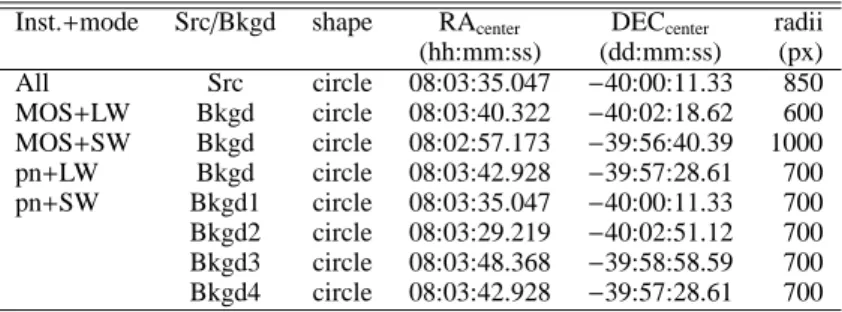
Table 2. Regions used for extracting source and background data from EPIC instruments.
Inst.+mode Src/Bkgd shape RAcenter DECcenter radii
(hh:mm:ss) (dd:mm:ss) (px) All Src circle 08:03:35.047 −40:00:11.33 850 MOS+LW Bkgd circle 08:03:40.322 −40:02:18.62 600 MOS+SW Bkgd circle 08:02:57.173 −39:56:40.39 1000 pn+LW Bkgd circle 08:03:42.928 −39:57:28.61 700 pn+SW Bkgd1 circle 08:03:35.047 −40:00:11.33 700 Bkgd2 circle 08:03:29.219 −40:02:51.12 700 Bkgd3 circle 08:03:48.368 −39:58:58.59 700 Bkgd4 circle 08:03:42.928 −39:57:28.61 700 Notes. Here, 1 px=0.05′′
. The source position is from the Hipparcos catalog (cf. Simbad). The background regions Bkgd 2 to 4 were used for Revs. 0636+0795+0980+1343, Revs. 0903+1071+1096, and Revs. 1620+1814+1983, respectively. In all other cases, the background region Bkgd1 was used.
to 8.9×1019cm−2(Diplas & Savage, 1994), and the abundances of the absorption and emission components are assumed to be equal. Adding a fifth thermal components (e.g. at 1 keV) does not significantly improve the fit, and we thus sticked to the deci-sion of using 4 components.
After the best-fit temperatures and absorptions were found, we investigated the impact of using non-solar abundances. We began by keeping the helium abundance to 2 times solar (Repolust et al., 2004), and let the nitrogen and oxygen abun-dances vary. We perfom such a simultaneous fit to all available EPIC spectra of each revolution. A few conclusions could be drawn from this trial. First, the pn spectra obtained in Large Window mode with the Medium filter (Revs 0156 and 0552, and second pn observation of Revs 535, 538 and 542) are clearly de-viant from other data, showing the impact of pile-up. Since all other data (pn or MOS, LW or SW modes with Thick filter) over-all agree with one another, we only discarded the pn data taken with Medium filter from further analysis. Second, the absorp-tions and temperatures of the fits do not vary much: we therefore fixed them to kTi of 0.09, 0.27, 0.56 and 2.18 keV and NH,i of
0.1, 0.1, 0.71, 0. ×1022cm−2. Finally, the origins of the high χ2
can be better pinpointed. On the one hand, MOS and pn data do not always agree, especially at 0.4 keV (see Fig. 1). This explains why some fits deviate from the mean behaviour: Revs 0731 and 1071 only provided pn data, while Revs 0156 and 1164 con-sist only of MOS data. This difference between MOS and pn is probably due to remaining cross-calibration problems, not pile-up since ζ Ppile-uppis is far from the pile-pile-up limit for data taken in SW mode with the Thick filter. On the other hand, all three in-struments (MOS1, MOS2, and pn) sometimes display δχ2of the
same sign. This is often the case near strong lines, which points toward two explanations: (1) atomic parameters are imperfect (even for APEC - Fig. 1 shows two examples: at 1.24 keV, there is flux in the data but not the model - a line is probably missing; at 1.5keV, there is a line in the model but not the data) and (2) the asymetric line shape of ζ Puppis influence even EPIC data. We cannot do much for the former, and the latter will actually be studied in detail in the third paper of this series - it is thus beyond the scope of this contribution.
The next step is to free more abundances, but this could yield erratic and/or problematic and/or not better results. For exam-ple, the carbon abundance clearly gets unrealistic (whether freed last or first). Indeed, low-resolution, broad-band spectra such as those taken by EPIC yield few constraints on the carbon abun-dance and, as often happens with such data, the fitting proce-dure favors high values of carbon enrichment, whatever its ac-tual value. From previous studies, it is well known that
nitro-10−4 10−3 0.01 0.1 1 10 normalized counts s −1 keV −1
Rev 1983: Nh and kT fixed
1 10 0.5 2 5 −100 −50 0 50 sign(data−model) × ∆ χ 2 Energy (keV)
Fig. 1. The EPIC pn (top, in green) and MOS (bottom, in red and
black) data of Rev. 1983 superimposed on the best-fit model.
gen is overabundant in ζ Puppis, and carbon may be subsolar (e.g. 0.35 times solar in Pauldrach et al. 2001 and 0.6 times so-lar in Oskinova et al. 2007). However, reported abundances vary quite a lot in literature (see other examples below) and, follow-ing Zhekov & Palla (2007), we decided to keep it to solar as for other non-constrained elements. For other elements, freeing the abundance may not improve the fitting quality or may not yield abundances significantly non-solar: this was the case of magne-sium, sulphur, iron and neon when released one after another. The silicon abundance stays close to solar but does improve the χ2, it was thus allowed to vary together with He, N, and O.
The best fit results are shown in Table 3. The parameter er-rors are taken from the raw fitting results of Xspec (i.e. these 1-σ errors are “calculated from the second derivatives of the fit statistic with respect to the model parameters at the best-fit”, and are indicative, see Xspec manual). No error is provided for the fluxes. We could indeed use the relative error on count rates, which would yield relative errors in the 0.1–0.3% range due to the sole Poisson noise. However, relative flux differences be-tween MOS and pn calibrations amount to about 1% in the soft energy band (where they are maximum), and the use of other similar models also yield 1% relative errors. Fluxes should there-fore be considered as determined to 1/100, not 1/1000, uncer-tainties.
Note that the listed parameters should not be over-interpretated: they simply represent a convenient way of well fit-ting the data, no more no less. The abundances, in particular, are
Ya¨el Naz´e et al.: A detailed X-ray investigation of ζ Puppis
indicative, high-resolution data providing much more stringent constraints (see Paper III). It is for example interesting to note that freeing all abundances at the same time could lead to a better χ2 but to totally erratic and unrealistic abundances (carbon
be-coming largely overabundant, nitrogen being solar). This being kept in mind, it is quite remarkable that our results, which should be considered as indicative only, agree rather well with previous abundance determinations. The helium abundance of ζ Puppis was found to be 1.2 and 3.4 times solar4 by Pauldrach et al. (2001) and Oskinova et al. (2006), respectively, and we found an average value of ∼2 (though this abundance is only weakly constrained in EPIC spectra). The nitrogen abundance was deter-mined to be 1.7, 6, and 8 times solar by Zhekov & Palla (2007), Oskinova et al. (2006), and Pauldrach et al. (2001), respectively, and we found again an average value of ∼4. The oxygen abun-dance is the least constrained of all, with values of 0.75, 1.6, and even 0.16 times solar reported by Pauldrach et al. (2001), Oskinova et al. (2006), and Zhekov & Palla (2007), respectively. The latter agrees well with our value, but it is formally uncon-strained since its error was 0.23. Our silicon determination also agrees well with the value found by Zhekov & Palla (2007).
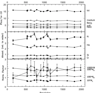
A few general conclusions can be drawn. The dominant components are those with temperatures of 0.09, 0.27 keV, and 0.56 keV (providing 20%, 43%, and 35% of the to-tal flux, respectively), corroborating the conclusion found by Zhekov & Palla (2007), with a different formalism, that cool plasma dominates in ζ Puppis. The flux and spectral pa-rameters do not vary much, the largest variations are ob-tained when only one instrument is available (e.g. Rev. 0156, where the pn data are discarded because of the piled-up as-sociated with the Medium filter). Fluxes (and their associ-ated dispersions) in the total (0.3–4. keV), soft (0.3–0.6 keV), medium (0.6–1.2 keV), hard (1.2–4. keV), and Bergh ¨ofer’s (0.9– 2. keV) bands5are 15.3±0.4, 4.15±0.14, 8.07±0.26, 3.06±0.09, 5.67±0.17 ×10⁻¹²erg cm−2s−1, respectively. Dispersions
typi-cally amount to 3%, slightly larger than the typical 1% error, and a shallow decreasing trend is detected, with a decrease of only ∼5% in flux since Rev. 0156. Such a decreasing trend is rem-iniscent of aging detector sensitivity problems, and we cannot exclude this possibility on the sole basis of the XMM-Newton dataset.
4. Wind profiles
Cohen et al. (2010) reported small variations of the line pro-files with wavelength, due to the energy-dependent opacity of the cool wind. However, the Chandra observation that they used was relatively short, hence subject to a much higher noise on the spectrum than for our data, and it is also rather insensitive to wavelengths >20Å, where the effect is expected to be the largest. We therefore re-investigate here the issue using the combined RGS spectrum, which has a better signal-to-noise ratio and ex-tends beyond 20Å.
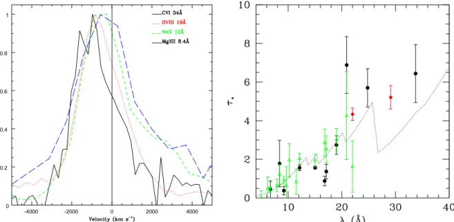
The left panel of Fig. 3 shows the observed Lyman α lines, in velocity space. For the figure, the lines were approximately continuum-subtracted and normalized to have a peak amplitude unity, to highlight their differences. Neighbouring lines can be seen for some of these Lyman α lines as bumps in the blue or red wings. Note that we do not show the N vii Lyα line as it is
4 As in Xspec: abundances are in number, relative to hydrogen, and
relative to solar.
5 For more details on the choice of energy bands, see Paper II.
0 500 1000 1500 2000 0 1 2 3 Revolution 1 2 3 4 5 O He N Si 0 500 1000 1500 2000 5 10 15 20 tot soft medium hard Berg.
Fig. 2. Spectral parameters as a function of Revolution number.
blended with a N vi line. The variations with wavelength are ob-vious, as the peak velocity clearly appears less blueshifted for the short-wavelength lines. The comparison of width and skew-ness is more difficult by eye, as the RGS resolution broadens the short-wavelength lines in velocity space, blurring the trends.
To quantify the wavelength variations, we fit the lines with the same models6as Cohen et al. (2010), to ensure homogeneity.
Results are provided in Table 4: the first two columns identify the considered line, the next three columns define the line shape (characteristic continuum optical depth τ∗, radius R∗for the
on-set of the X-ray emission, and the strength of the line), and the last two column provides details of the line ratios in the He-like fir triplets.
Several things must be noted. First, in two cases (the He-like triplets of N and O), resonance scattering was needed to achieve a good fit. Second, the Lyman α line of nitrogen is blended with a line from N vi. We fit these two lines together, assuming that the line profile parameters are identical: keeping them independent yields unrealistic results (τ∗∼0) for the weak N vi line, and the
lines are so blended that little independent information is avail-able, explaining the apparently strange results for the weakest line. The achieved fit of the nitrogen blend is far from perfect, however (χ2∼2). Third, the iron line at 15Å is not very well
fit-ted (χ2 ∼2), despite our efforts. It seems that line blends (there are numerous Fe xviii lines in the neighbourhood) affect the pro-file: though these lines are weak, the very low noise of our data reveals their impact, which was not obvious in the Chandra data. Finally, the fitting was done using a single terminal velocity for the wind (2250km s−1, Puls et al. 2006), a β=1 exponent for the velocity law, and a power law of zero slope to represent the con-tinuum.
6 Wind profile models for Xspec are available on
http://heasarc.nasa.gov/xanadu/xspec/models/windprof.html
Y a ¨el N az ´e et al .: A d et ai le d X -r ay in v es tig at io n o f ζ P u p p is 0538 0.060±0.004 1.15±0.02 1.85±0.02 1.93±0.52 2.32±0.08 4.19±0.17 0.256±0.007 0.80±0.02 5.17 (268) 15.2 4.02 7.98 3.13 5.71 0542 0.058±0.003 1.18±0.02 1.89±0.02 1.84±0.48 2.21±0.08 4.18±0.16 0.262±0.007 0.77±0.02 5.76 (276) 15.7 4.20 8.31 3.16 5.85 0636 0.059±0.004 1.21±0.02 1.79±0.02 2.25±0.65 2.17±0.09 4.15±0.18 0.263±0.008 0.80±0.02 3.37 (257) 15.8 4.34 8.38 3.09 5.77 0731 0.070±0.006 1.23±0.03 1.73±0.03 2.11±0.64 2.54±0.11 4.61±0.26 0.231±0.008 0.80±0.03 2.92 (111) 15.0 4.19 7.78 2.98 5.48 0795 0.072±0.005 1.23±0.02 1.88±0.02 1.08±0.64 2.33±0.09 3.67±0.17 0.258±0.008 0.70±0.02 2.78 (249) 16.1 4.45 8.51 3.09 5.86 0903 0.069±0.005 1.13±0.02 1.75±0.02 1.80±0.59 2.38±0.09 3.78±0.18 0.241±0.008 0.78±0.02 3.06 (259) 14.9 4.13 7.78 2.97 5.49 0980 0.064±0.004 1.12±0.02 1.80±0.02 2.18±0.49 2.39±0.08 4.02±0.15 0.259±0.007 0.75±0.02 3.33 (414) 14.8 4.00 7.74 3.04 5.53 1071 0.062±0.008 1.27±0.04 1.71±0.04 2.08±1.11 2.37±0.16 4.59±0.35 0.234±0.012 0.81±0.04 2.02 (96) 15.3 4.24 8.09 2.96 5.57 1096 0.056±0.003 1.17±0.02 1.78±0.02 2.06±0.42 2.09±0.06 4.21±0.13 0.273±0.006 0.76±0.02 6.16 (285) 15.6 4.35 8.24 3.02 5.66 1164 0.068±0.005 1.14±0.02 1.82±0.02 1.39±0.60 2.45±0.09 3.62±0.17 0.274±0.009 0.63±0.02 5.25 (156) 14.9 4.00 7.90 3.00 5.52 1343 0.066±0.003 1.17±0.02 1.76±0.01 2.06±0.40 2.33±0.06 3.74±0.12 0.265±0.006 0.77±0.02 5.36 (289) 15.2 4.16 8.05 3.01 5.59 1620 0.063±0.003 1.19±0.02 1.87±0.01 1.79±0.38 2.31±0.06 3.72±0.11 0.264±0.005 0.74±0.02 6.97 (291) 15.6 4.09 8.32 3.14 5.83 1814 0.056±0.003 1.09±0.01 1.74±0.01 2.11±0.36 2.21±0.06 4.06±0.12 0.269±0.005 0.76±0.01 6.77 (300) 14.7 3.98 7.73 2.95 5.43 1983 0.066±0.003 1.14±0.01 1.81±0.01 2.07±0.32 2.45±0.05 4.02±0.11 0.257±0.005 0.77±0.01 7.90 (306) 14.9 4.01 7.79 3.06 5.56
Notes. The fitted model has the form tbabs ×Pvphabs × vapec, where the interstellar absorption was fixed to 8.9×1019cm−2, and the additional absorbing columns and temperatures are fixed to NH,1,2,3,4=0.10, 0.10, 0.71, 0.×1022cm−2and kT1,2,3,4=0.09, 0.27, 0.56, 2.18 keV, respectively. Abundances are by number relative to hydrogen and relative to solar.
Ya¨el Naz´e et al.: A detailed X-ray investigation of ζ Puppis
As it is always compatible with zero and as it yields no im-provement of the fits, no global line profile shift was applied, except for the iron lines near 17Å where the improvement is sig-nificant with a shift of only –15±2 km s−1. Wavelength shifts
between instruments/orders were envisaged, but they yielded er-ratic results generally without improvement of the fit, sometimes large values (incompatible with wavelength calibration reports) for example for the iron line at 15Å, values compatible with zero within 3 sigma, and values for one instrument/order compatible with those of another instrument/order within 3 sigma. Cross-correlation also suggests null shifts between exposures and be-tween different instrument/order combinations of the same ex-posure. Due to the broadness of its lines, ζ Puppis is indeed not the best source to find such shifts: to do so, the XMM-Newton calibration team uses sources with unresolved X-ray lines.
As shown in the right panel of Fig. 3, the optical depth varies with wavelength. Our fitting thus confirms the Cohen et al. (2010) preliminary results by extending them to longer wave-lengths and by decreasing the noise on most lines (except the bluest ones). The wind of ζ Puppis therefore is unlikely to be composed of clumps which are fully opaque at all wavelengths, as had been suggested for some porosity models. Indeed, op-tically thick clumps should produce a grey opacity that would solely be determined by the geometry of the clumps. In princi-ple, these optical depth variations may be used to constrain the mass-loss rate, for a given star+wind model. This was attempted in Cohen et al. (2010), and they found that a reduced mass-loss rate with non-solar abundances provided the best-fit results. For comparison purposes, the same theoretical opacity is shown in Fig. 3 with a dotted line: below 20Å, it indeed provides a good fit, but for larger wavelengths, the agreement is less good be-cause of the nitrogen edge at 26Å - an edge which appears very strong as the nitrogen abundance is enhanced for ζ Puppis. This discrepancy may be solved by adapting the value of the abun-dances and mass-loss rate of ζ Puppis, but this is beyond the scope of this paper. Clearly, additional modelling is needed to reproduce the full behaviour of ζ Puppis in X-rays (and this will be done in Paper III).
In contrast, the onset radius appears remarkably stable and confined in the 1–1.5 R∗range, which is quite usual in massive
stars (G¨udel & Naz´e, 2009, and references therein). The sole ex-ceptions are the Nitrogen triplet and Lyα lines, but it would not be surprising that, as these lines have emissivities that peak at rather low temperatures, it simply indicates a formation further out in the wind.
5. Conclusion
In the past decade, about 1Ms of data were obtained by
XMM-Newton on ζ Puppis. Of these, about 30% is strongly affected by
flares, reducing the useful exposures to 579ks for EPIC-MOS, 477ks for EPIC-pn, and 751ks for RGS. A variety of modes was used, the most reliable being the SW+Thick Filter mode; the use of the medium filter yielded piled-up data, while the data taken in LW+Thick Filter mode do not appear significantly different from those obtained with SW+Thick Filter mode. Attention was paid to this problem, notably by choosing similar extraction regions for all datasets and using only single events.
Broad-band EPIC data taken with the Thick filter were an-alyzed using absorbed optically-thin thermal emissions. Four temperatures are needed to reproduce in a reasonable way the data. Note that the fits are not formally acceptable, but that (1) instruments do not always agree with one another and (2) the
re-duced noise amplifies the limitations due to the imperfect atomic parameters and standard line profiles. Nevertheless, the EPIC spectra appear remarkably stable over the decade of observa-tions, with only 3% dispersions around the average fluxes. A de-tailed variability study, based on lightcurves, will be presented in Paper II.
The combined high-resolution RGS spectrum confirms that the X-ray line profiles vary with wavelength. Fitting individual line profiles using a wind model yields similar onset radius for the X-ray emission, but wind continuum opacities depending on wavelength. This is simply due to the fact that the cool ab-sorbing clumps in the wind are not fully optically thick at all wavelengths, though further modelling is needed in order to ad-equately reproduce the opacity variations.
Acknowledgements. YN acknowledges L. Mahy for his help with CMFGEN,
and the XMM-Newton helpdesk for interesting discussions about the data. YN and GR acknowledge support from the Fonds National de la Recherche Scientifique (Belgium), the Communaut´e Franc¸aise de Belgique, the PRODEX XMM and Integral contracts, and the ‘Action de Recherche Concert´ee’ (CFWB-Acad´emie Wallonie Europe). CAF acknowledges support from the FNRS-Conacyt agreement, as well as from the ‘Programa de becas para la formac´ıon de j´ovenes investigatores de la DAIP-GTO’. ADS and CDS were used for preparing this document.
References
Berghoefer, T. W., Baade, D., Schmitt, J. H. M. M., Kudritzki, R.-P., Puls, J., Hillier, D. J., & Pauldrach, A. W. A. 1996, A&A, 306, 899
Cassinelli, J. P., Miller, N. A., Waldron, W. L., MacFarlane, J. J., & Cohen, D. H. 2001, ApJ, 554, L55
Cohen, D. H., Leutenegger, M. A., Wollman, E. E., Zsarg´o, J., Hillier, D. J., Townsend, R. H. D., & Owocki, S. P. 2010, MNRAS, 405, 2391
Conti, P. S., & Leep, E. M. 1974, ApJ, 193, 113 Diplas, A., & Savage, B. D. 1994, ApJS, 93, 211
Feldmeier, A., Oskinova, L., & Hamann, W.-R. 2003, A&A, 403, 217 G ¨udel, M., & Naz´e, Y. 2009, A&A Rev., 17, 309
Harries, T. J., & Howarth, I. D. 1996, A&A, 310, 533
Howarth, I. D., Siebert, K. W., Hussain, G. A. J., & Prinja, R. K. 1997, MNRAS, 284, 265
Kahn, S. M., Leutenegger, M. A., Cottam, J., Rauw, G., Vreux, J.-M., den Boggende, A. J. F., Mewe, R., G ¨udel, M. 2001, A&A, 365, L312
Kramer, R. H., Cohen, D. H., & Owocki, S. P. 2003, ApJ, 592, 532
Leutenegger, M. A., Owocki, S. P., Kahn, S. M., & Paerels, F. B. S. 2007, ApJ, 659, 642
Ma´ız Apell´aniz, J., Alfaro, E. J., & Sota, A. 2008, poster presented at IAU Symposium 250, arXiv:0804.2553
Meynet, G., & Maeder, A. 2000, A&A, 361, 101 Moffat, A. F. J., et al. 1998, A&A, 331, 949
Oskinova, L. M., Feldmeier, A., & Hamann, W.-R. 2006, MNRAS, 372, 313 Oskinova, L. M., Hamann, W.-R., & Feldmeier, A. 2007, A&A, 476, 1331 Owocki, S. P., & Cohen, D. H. 2001, ApJ, 559, 1108
Pauldrach, A. W. A., Hoffmann, T. L., & Lennon, M. 2001, A&A, 375, 161 Penny, L. R. 1996, ApJ, 463, 737
Petrenz, P., & Puls, J. 1996, A&A, 312, 195
Puls, J., Markova, N., Scuderi, S., et al. 2006, A&A, 454, 625 Repolust, T., Puls, J., & Herrero, A. 2004, A&A, 415, 349 Schaerer, D., Schmutz, W., & Grenon, M. 1997, ApJ, 484, L153 van Leeuwen, F. 2007, A&A, 474, 653
van Rensbergen, W., Vanbeveren, D., & De Loore, C. 1996, A&A, 305, 825 Walborn, N. R. 1972, AJ, 77, 312
Zhekov S.A., & Palla, F. 2007, MNRAS, 382, 1124
-4000 -2000 0 2000 4000 0 0.2 0.4 0.6 0.8 1
Fig. 3. Left: Line profiles in velocity space, of the observed Lyman α lines. Right: Variations of the mean optical depth τ∗ with
wavelength. Results from this work are shown with filled circles and hexagons - the latter for fits including resonance scattering, while Cohen et al. (2010) results are displayed with empty triangles. The Cohen et al. theoretical absorption is shown by a dotted line.
Table 4. Parameters of the wind profiles.
Ion λ τ∗ R0/R∗ norm G=(f+i)/r P = φ∗/φc
(Å) (10−4ph cm−2s−1) (in 104) Si xiii-tr 6.7 0.40.8 0.0 1.0 1.2 1.0 1.15 1.18 1.12 0.68 0.79 0.55 0.0002 0.0005 0.0001 Mg xii-Lyα 8.4 1.83.0 0.9 1.2 1.5 1.0 0.30 0.32 0.27 Mg xi-tr 9.2 0.40.6 0.2 1.4 1.5 1.3 2.05 2.07 2.02 0.73 0.78 0.67 0.004 0.005 0.003 Ne x-Lyα 12.1 1.61.7 1.4 1.5 1.6 1.4 3.03 3.06 3.00 Fe xvii 15.0 1.61.6 1.5 1.7 1.7 1.6 6.36 6.45 6.28 Fe xvii 16.8 0.91.1 0.7 1.5 1.6 1.5 2.69 2.72 2.66 Fe xvii 17.1 1.41.7 1.1 1.5 1.6 1.4 4.08 4.12 4.06 O viii-Lyα 19.0 2.72.9 2.3 1.0 1.3 1.0 4.62 4.72 4.53 N vii-Lyβ 20.9 6.98.3 5.6 1.3 1.9 1.0 1.80 1.85 1.75 O vii-tr 21.7 4.34.6 4.0 1.3 1.6 1.0 7.31 7.39 7.23 1.06 1.07 1.02 3.1 3.8 2.4 N vii-Lyα 24.8 5.76.7 4.7 2.1 3.2 1.1 6.16 5.84 6.48 N vi-tr 29.1 5.25.7 4.6 2.7 2.8 2.5 18.7 18.9 18.6 1.18 1.19 1.15 7.6 9.3 5.9 C vi-Lyα 33.7 6.47.9 5.4 1.1 1.7 1.0 1.24 1.29 1.20
Notes. tr refers to He-like triplets, and Ly to Lyman lines. Shifts and line profiles are identical for all lines of the doublets (Lyman α, Lyman
β, Fe xvii doublet at 17.1Å) and triplets; the line ratio in doublets is fixed to the ratio of maximum emissivities. For the N vi triplet, resonance scattering parameters are τ0
∗>56, βsob<0.28; for the O vii triplet, resonance scattering parameters are τ0∗>18, βsob= 1.42.00.9.