HAL Id: hal-01981401
https://hal.archives-ouvertes.fr/hal-01981401
Submitted on 15 Jan 2019
HAL is a multi-disciplinary open access
archive for the deposit and dissemination of
sci-entific research documents, whether they are
pub-lished or not. The documents may come from
teaching and research institutions in France or
abroad, or from public or private research centers.
L’archive ouverte pluridisciplinaire HAL, est
destinée au dépôt et à la diffusion de documents
scientifiques de niveau recherche, publiés ou non,
émanant des établissements d’enseignement et de
recherche français ou étrangers, des laboratoires
publics ou privés.
Evaluation of Water Heaters Control Strategies For
Electricity Storage And Load Shedding At National
Scale
Baptiste Béjannin, Thomas Berthou, Bruno Duplessis, Dominique Marchio
To cite this version:
Baptiste Béjannin, Thomas Berthou, Bruno Duplessis, Dominique Marchio. Evaluation of Water
Heaters Control Strategies For Electricity Storage And Load Shedding At National Scale. 4th
Build-ing Simulation and Optimization Conference, Cambridge, UK, Sep 2018, Cambridge, UK, United
Kingdom. �hal-01981401�
Evaluation of Water Heaters Control Strategies For Electricity Storage And Load Shedding
At National Scale
Baptiste Béjannin
1, Thomas Berthou
1, Bruno Duplessis
1, Dominique Marchio
11
MINES ParisTech, PSL Research University, Centre d’efficacité énergétique des systèmes
Abstract
The objective of this study is to assess the impact of storage and cut-off scenarios on electric water heaters at national scale. It provides directions for future optimization on the French electric load curve.
Thanks to accurate modellings of drop-off scenarios, it is possible to simulate hundreds of hot water tanks which represent a country’s stock. The model of water heaters is adequate for an accurate assessment of domestic hot water (DHW) parameters - draw-off temperature, end user comfort and the influence of the temperature sensor controlling on/off sequences -, while reducing the computation time. The electrical water heaters (EWH) are parameterized using long-term sales statistics combined with a water drop-off time of use survey to represent the national diversity.
Within the scope of reducing the power demand and maintaining the comfort of the consumers or, on the contrary, storing the maximum energy possible during a certain period of the day; we simulate - with a representative panel of EWH - two scenarios which consist in:
Turning the EWH on to increase national electric demand for a short time,
Cutting the EWH off to reduce national electricity demand for a short time.
Introduction
Renewable energies have taken on significant importance in the energy mix. To support the integration of these new intermittent energy sources, larger flexibility from the electrical grid is needed. EWH can be viewed as an opportunity to increase this flexibility on a large scale. Indeed, thanks to their ability to store energy, they can be switched off - for load shedding purpose - or switched on - for storage purpose - without affecting the comfort of the consumers.
Several papers have already studied the control of a EWH stock. The aim is whether to decrease the maximum of the demand power or to minimize the consumed energy while maximizing the comfort of the consumers. For example, Atikol (2013) suggests forcing some water heaters to be turned on before or after the night peak consumption. Dolan (1996) creates a turning load shedding during all the day. Rautenbach (1996) and Sepulveda (2010) obtain a diminution of the power peak
respectively with the gradient method and binary particle swarm optimization. In most of those papers, the comfort assessment is rather limited. In fact, it is even omitted in the optimisation process. The originality of our research paper lies in including user comfort in the assessment parameters such as the energy stored in the tanks. Moreover, in order to launch optimization processes on thousands of devices, this paper introduces a fast running model of EWH which is compared to a validated model - Koch (2012).
In this paper, we aim thus to evaluate the effect of two control scenarios on an EWH stock: a “storage” scenario and a “load shedding” scenario. To this purpose, indicators such as comfort of consumers, energy consumption and load curve are assessed based on a dynamic simulation of thousands of water heaters. The first section of this paper explains how we build an EWH population representative of French stock and the second section proposes a fast running model of EWH , which is adapted not only to large-scale simulations, but also to DHW stock modelling and EWH control optimisation. In the third part of this paper we evaluate the potential of control scenarios whether by power storing or load shedding. Finally, thanks to these simulations relying on two different controls of EWH, we provide an assessment of the flexibility brought to the grid.
Building of an electric water heaters stock
model
In order to represent EWH consumption of all French dwellings consuming electricity to heat their domestic hot water (DHW), we build a population of more than 4000 housings equipped with EWH. The main diversity factors among this population are either sizing parameters - the capacity of the EWH tanks - or commands as the water draw-off scenarios and the ON/OFF remote control from the grid. Therefore, the first step in defining a realistic EWH stock consists in gathering or rebuilding these diversity factors.
Capacity distribution of DHW tanks
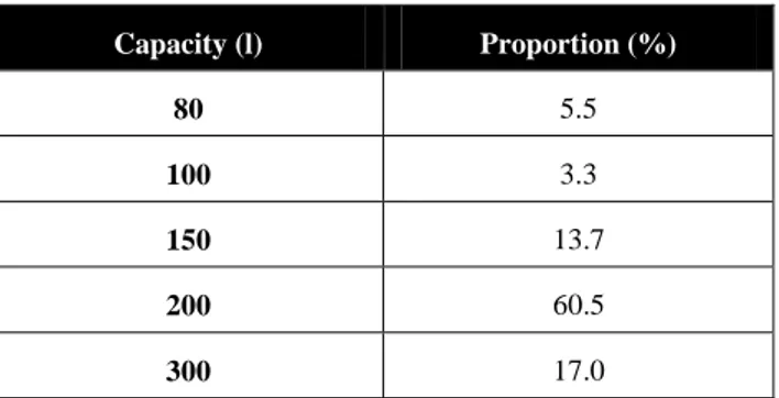
The distribution of EWH tanks capacity is taken from Kemna (2007) and showed in Table 1.
Proceedings of BSO 2018: 4th Building Simulation and Optimization Conference, Cambridge, UK: 11-12 September 2018
The capacities of the EWH are related to the area of the dwellings - eg. the 5.5% smallest dwellings are equipped with 80 l EWH.
Table 1: Distribution of EWH in France
Capacity (l) Proportion (%) 80 5.5 100 3.3 150 13.7 200 60.5 300 17.0 DHW draw-off scenarios
In order to build realistic DHW draw-off scenarios, we use data from the so-called “schedule survey” processed by French National Institute of Statistics and Economic Studies - INSEE (2012). It contains 19 000 time schedules filled out by French people describing their daily activities with a 10 minutes time step. Thanks to this data, Berthou (2016) obtains realistic DHW draw-off scenarios.
Simulation of the existing control scenarios
In France, a vast majority of housings with EWH are supplied with a Time Of Use (TOU) tariff electricity usually called “peak/off-peak hours” tariff. This tariff drops during the off-peak hours which is a period of 8 hours. In order to take advantage of this TOU tariff, most of the EWH are synchronised with its variation: EWH are switched off during peak hours and can be turned-on only during off-peak hours.
There is no public data to determine the actual distribution of TOU scenarios across France. Such a scenario depends on the consumption site and is managed by the distribution grid operator. Off-peak hours can be in one block during the night (for 8 hours) or split between the night (5 hours) and the day (3 hours). Barely 15% of the electric water heater dwellings do not have any off-peak hour’s scenario. In Berthou (2016), a calibration process allowed to identify an “off-peak hours” scenario to fit the current real load curve of French EWH (Figure 1
)
. This scenario is repeated every day. A “no control” scenario is also used hereafter for evaluation purposes. It consists of letting the EWH function exclusively based on the DHW drop-off. Figure 1 shows that the 15% of EWH dwellings which do not have any off-peak hours scenario are visible - anytime, there is at least 15% of the stock that is allowed to function.Figure 1: Current “off peak hours” scenarios: proportion of French EWH allowed to operate along the
day
With these three diversity factors, we are now able to create a realistic panel of more than 4000 EWH, which is representative of French EWH stock. The thermodynamic water heaters are not considered in this study since they represent less than 5 % of the stock.
Development of a fast running model of
EWH
To be suitable for control, the EWH model must represent both power demand and actual DHW temperature. Nevertheless, it must be as “simple” as possible in order to make parameterisation and simulation as fast as possible.
Model requirements
To meet the study objective, three constraints on the EWH models have been identified.
Firstly, the comfort of all the consumers at any time has to be evaluated. As the comfort is directly linked to the temperature of the water going out of the tank, we need to get the most realistic assessment of the water temperature at the tank outlet. Secondly, we also have to ensure a good accuracy in energy and power demand evaluation. This will make sure that we obtain a correct representation of the demand power at an aggregated scale. Therefore, the two values must be part of the model outputs. They are directly related to the mean temperature - which represents the energy stored in the tank - and the temperature used as actuating value for the EWH controller - the temperature sensor of the controller is located in the lower half of the tank.
Finally, as we want to simulate more than 4000 water heaters over a few days - typically a week -, the calculation time must be reasonable.
Reference model from the literature
Koch (2012) proposes a one-dimension model of EWH that gives good results in terms of temperature and power demand simulation. This model approximates EWH to a cylinder as follows:
The water tank is discretized in several layers - whose number may vary from ten to one hundred - which are considered as homogeneous temperature zones and analysed individually based on mass and energy balances
The temperature of each water layer depends on various terms such as:
o Heat diffusion - conduction and convection - between the layers
o The “plug flow” term resulting from water draws,
o Heat losses to the environment, o Heating element - power injection.
The power supplied in the lower fifth of the tank. The EWH is turned on when the volume-controlled temperature is under 57°C and turned off when it is over 63°C. Between those two temperatures, the EWH remains in the same working condition. This model describes accurately the evolution of temperature and power of the water heater through the day. It has been validated by comparison with experimental data - Pfeiffer (2011). As in Koch (2012), we run simulations of EWH by using 10 layers to discretize the tank and a 10-second time step. Figure 2 shows the temperature in every layer for one EWH during two usual days - the water draw-off is in green.
Figure 2: Temperatures in each layer calculated with
(Koch 2012) model - one water heater and water
drop-off (green)
After each heating period, we observe that the water temperature gradient is reversed. Indeed, this unexpected behaviour has already been highlighted by the author and is a limit of the model. Nevertheless, this limit does not compromise an evaluation of users’ comfort and, above all, the model gives excellent evaluations of the energy and power demand - Pfeiffer (2011). This makes us consider this model as a reference for our future work. Figure 3 shows the mean power demand during two days for a stock of 4143 EWH based on this reference model and without any control from the grid - the average water draw-off is in green.
Figure 3: Mean power demand of French EWH stock - reference model
The main disadvantage of this model comes from the constraint on the simulation time step - 10 seconds - which causes time-consuming simulations. Indeed, this time step cannot be increased without creating numerical incoherence coming from the convection term and due to the explicit formulation of the differential equations. Consequently, a better model seems to be one with similar results to Koch (2012), but with a longer time step.
Fast running model for large-scale simulations
As previously mentioned, numerical incoherences come from the convection term. This is why we implement a mixing algorithm that substitutes the convection term. Energy and mass balances in each layer are first simulated without the convention term. Then, at each time step we check if the water temperature gradient in the tank is correctly oriented - respects the physical stratification. If not, the affected water layers are mixed to get the expected behaviour of the stratified water tank. Finally, this fast running model runs with a time step of 2,5 minutes which seems to be a good trade-off between calculation time management and accuracy in considering small water draw-off.
Validation of the fast running model
In order to validate our approach, the mean temperature and power calculated by the fast running model are compared to the values given by the reference model Koch (2012) over a one-week simulation. Despite some periods of dephasing between outputs of the two models - Figure 4 and Figure 5 -, we observe a very satisfying match at the stock scale - Figure 6 and Figure 7.
Figure 4: Mean temperature from fast running and reference models - one 300l EWH
Figure 5: Power demand from fast running and reference models - one 300l EWH
Indeed, the inter-correlation coefficient R² - defined in (1) - between the DHW mean water temperature of the fast running model and that of the reference model - presented on Figure 6 - is equal to 0,99.
In (1), cov(X,Y) is the covariance of the two variables X and Y; and var(X) refers to the variance of the variable X.
Figure 6: Mean temperature in DHW tanks stock from fast running and reference models
Figure 7 shows the mean power demand of both models.
R² between these two time series reaches 0,92 and
relative deviation does not exceed 20 % locally - Figure 8
.
Figure 7: Mean power demand in DHW tanks stock from fast running and reference models
Furthermore, an in-depth analysis shows that the mean power difference is -0,3 % on average - i.e. the bias is marginal - and that the standard deviation between both times series is 9,7 % as presented in Figure 9.
Figure 8: Comparison of the power values from fast running and reference models
Figure 9: Standardised histogram of the deviations between fast running and reference models
In terms of computing time, our fast running model needs 8 minutes to simulate more than 4000 water heaters during 12 days, whereas the reference model Koch (2012) needs 46 minutes - which means a time decrease of more than 82 % - in the same conditions. This significant improvement opens the door to the assessment and the optimisation of various control strategies.
Results
Simulation and evaluation of the potential of power storing
The first analysis consists in assessing how much energy can be stored by a EWH stock during one hour.
As a reference for this study, we consider a EWH stock that is subject to an off-peak hour scenario - as mentioned previously and showed in Figure 1. From this “off peak hours” scenario, we simulate a period of storage by allowing the whole stock of EWH to be switched on during one hour in the afternoon - from 2pm to 3pm. We choose this period as it corresponds to an off peak period both for water draw-off and for EWH. In other words, this “storage” scenario consists in enabling the EWH stock to operate forward compared to “off peak hours” scenario, which can help take advantage of a potential over production of electricity. Figure 10 presents the new operating schedule for EWH in the “storage” scenario framework.
Figure 10: Distribution of EWH allowed to operate in “storage” scenario
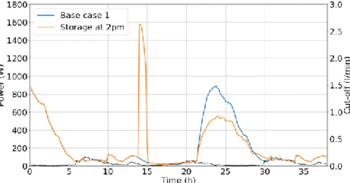
The base case in this scenario is the one where 85 % of the EWH are controlled - as it is shown in Figure 1 - and is called “Base case 1” in the remaining part of this paper.
Figure 11 shows that between 2pm and 3pm, 1,35 kWh are stored on average for a single water heater. The peak power of the night - 21h to 29h - is decreased from 770 W to 550 W on average on the stock, which represents a decrease of 28 %. Moreover, brought to national scale, this represents a storage of 14,85 GWh - France counts about 11 000 000 electric water heaters.
Figure 11: Mean Power demand in the two scenarios
In order to evaluate the resilience of the storage capacity supplied by the EWH stock, Figure 12 presents the mean temperature of all the tanks: 24 hours after the “storage” event, the state in terms of temperature - and thus the storage capacity of the stock - is recovered, which gives the opportunity for a further “storage” event.
Figure 12: Mean temperature in the two scenarios
Finally, by restarting the water heaters earlier in the afternoon, this scenario increases the comfort of the consumers - Figure 13. The discomfort is calculated using the proportion of EWH that delivers water at a temperature below 45°C.
Figure 13: Part of discomfort in the two scenarios
This storage scenario is interesting because it can decrease the discomfort of the consumers while decreasing the peak of the power demand in the night and not modifying the stock of water heaters 24 hours
after. However, during the 24 hours following the establishment of the storage scenario, the heat losses are 7,2% higher compared to the base case 1 - in the base case 1, the heat losses correspond to 1,2 kWh in 24h.
Simulation and evaluation of load shedding
The second scenario consists in estimating the impact of a “rotating load shedding” on the EWH stock during several hours.
As a reference for this case study, we consider a EWH stock without any control by the grid - as shown in Figure 3. This base case is called “Base case 2” in the remaining part of this paper.
In this paper, we look for a control strategy which could be suitable in French context: the load shedding order is applied during the national electric daily-peak period that has been identified by RTE - French electric grid company-, from 6 pm to 8 pm. In order to decrease significantly the national electric curve, the first idea is to turn off every EWH during the two hours.
First of all, Figure 14 shows the demand power in this case and in the base case 2 - without any control besides the regulation related to the water temperature of the tanks.
Figure 14: Mean power demand with turning-off every EWH during 2 hours
This scenario decreases the national electric curve during a daily-peak period, but the rebound generated after this period is unacceptable: the rebound after the cut-off reaches 700 W - whereas the peak of the day in the base case 2 is 500 W.
Based on these first results, we design a “rotating load shedding” scenario based on past experiments from Dolan (1996): it consists in alternatively switching off 25% of the EWH stock from 6 pm to 8 pm.
Figure 15 presents the mean power demand resulting from the “rotating load shedding” scenario and the reference one. As in the storage scenario and in order to evaluate the impact during a 24-hour period, the curve data covers the whole day until 6 pm the next day.
Figure 15: Mean power demand for turning load shedding scenario
During the load shedding event - from 6 pm to 8 pm -, the mean power is lower than in the base case 2. This is not surprising as 25 % of EWH stock is turned off. After 8 pm, after the end of the rotating load shedding, the mean power demand becomes higher than in the base case 2 but the rebound effect is softened. As the hot water stock has been reduced during two hours by the load shedding, a fraction of EWH is over consuming in comparison with the reference case during the hours following the “load shedding” experiment.
Figure 16 presents the mean temperature resulting from the two scenarios.
Figure 16: Mean temperature in the turning load shedding scenario
24 hours after the beginning of the experiment, the mean temperature is the same as in the reference model. This means that the “load shedding” scenario does not modify the stock - in terms of temperature - more than 24 hours after the load shedding event. Therefore, this scenario can be repeated every day.
Finally, the impact on the comfort of the consumers is also limited - less than 0,1 % for both scenarios.
Eventually, Table 2 shows the difference of energy consumption between the two scenarios and the maximum gap of the load curve. In order to appreciate the impact of our scenario at the French level, the results have been extrapolated from the EWH stock - as introduced in the first part - to the national scale by assuming a control of all French EWH by the grid.
Table 2: Energy impact of the turning load shedding scenario Periods 0am-6pm 6pm-8pm 8pm-6pm Difference of consumed energy (GWh) 0 -0.52 0.49
Maximum gap of the
load curves (MW) 0 -633.6 745.8
On the full period of the event - from 6 pm to 6 pm on the next day-, an amount of 30 MWh is saved thanks to this scenario, which is negligible compared to the overall consumption at national scale - barely 61 GWh in one regular day. The concomitant peaks are other parameters that are important to evaluate at the national grid level: for France, they refer to the power consumption at 9am and at 7pm, which are peak times on the French grid. This scenario decreases the night peak - at 7pm - by 19 MW which is barely marketable on the electricity balance market.
This turning load shedding scenario causes a shrinkage of the power demand during the daily-peak period - at 7 pm - without compromising the comfort of the consumers. Moreover, this scenario can be repeated every day without modifying the stock of EWH.
Conclusion
In this paper, a novel fast running model of EWH stock has been presented. Its results have been validated against literature.
Two scenarios have been simulated with this fast running model in order to estimate the potential of storage or load shedding of the French EWH stock. In both scenarios, the thermal state of the EWH stock is recovered 24 hours after the start of the control, which means that they could be applied every day without downgrading the DHW stock on the long term.
The first scenario shows that the only drawback of turning on all EWH of the stock for one hour in the afternoon is the increase of heat losses.
The second scenario offers a case of load shedding in order to decrease the power demand during the daily-peak period - around 7pm.
There are multiple directions to build on this novel development. One interesting direction for future research is to apply optimisation algorithms in order to create other control scenarios that maximize the load flexibilities on the grid. Moreover, regarding EWH modelling, the scenario of water-draws will be improved in the future in order to obtain more realistic drop-off. Indeed, the water flow may change according to the consumers' activity. Finally, with a time step of 2,5 minutes, the DHW scenario can be more precise. These limits leave room for improvement in further research.
Acknowledgments
The authors gratefully acknowledge the support provided by ADEME - Agence De l’Environnement et de la Maîtrise de l’Énergie - in the frame of “SmartGrid” Programmeof the Investments for the Future - PIA.
References
Atikol, Uğur. 2013. “A Simple Peak Shifting DSM (Demand-Side Management) Strategy for Residential Water Heaters.” Energy 62: 435-40. Berthou, Thomas, Bruno Duplessis, and Philippe
Rivière. 2016. “Modélisation Énergétique D’un Parc de Chauffe-Eau Électriques : Éléments de Validation.”
Dolan, P S, M H Nehrir, and V Gerez De. 1996. “Development of a Monte Carlo Based Aggregate Model for Residential Electric Water Heater Loads.” Electric Power Systems Research 36: 29-35.
INSEE. 2012. Enquête Emplois Du Temps.
Kemna, René, Martijn Van Elburg, William Li, and Rob van Holsteijn. 2007. “Eco-Design of Water Heaters.” Delft: Van Holsteijn en …: 154. Koch, S. 2012. Doctoral Thesis: Demand Response
Methods for Ancillary Services and Renewable Energy Integration in Electric Power Systems.
Pfeiffer, Martin, Göran Andersson Supervisor, and Dipl-Ing Stephan Koch Zurich. 2011. “Load Control Strategies for Electric Water Heaters with Thermal Stratification.”
Rautenbach, B., and I.E. Lane. 1996. “The Multi-Objective Controller: A Novel Approach to Domestic Hot Water Load Control.” IEEE
Transactions on Power Systems 11(4): 1832-37.
Sepulveda, Arnaldo et al. 2010. “A Novel Demand Side Management Program Using Water Heaters and Particle Swarm Optimization.” In 2010 IEEE
Electrical Power & Energy Conference, IEEE,