HAL Id: hal-00798070
https://hal.archives-ouvertes.fr/hal-00798070
Submitted on 7 Mar 2013
HAL is a multi-disciplinary open access
archive for the deposit and dissemination of
sci-entific research documents, whether they are
pub-lished or not. The documents may come from
teaching and research institutions in France or
abroad, or from public or private research centers.
L’archive ouverte pluridisciplinaire HAL, est
destinée au dépôt et à la diffusion de documents
scientifiques de niveau recherche, publiés ou non,
émanant des établissements d’enseignement et de
recherche français ou étrangers, des laboratoires
publics ou privés.
A comprehensive probabilistic model of chloride ingress
in unsaturated concrete
Emilio Bastidas-Arteaga, Alaa Chateauneuf, Mauricio Sánchez-Silva, Philippe
Bressolette, Franck Schoefs
To cite this version:
Emilio Bastidas-Arteaga, Alaa Chateauneuf, Mauricio Sánchez-Silva, Philippe Bressolette, Franck
Schoefs. A comprehensive probabilistic model of chloride ingress in unsaturated concrete. Engineering
Structures, Elsevier, 2011, 33 (3), pp.720-730. �10.1016/j.engstruct.2010.11.008�. �hal-00798070�
A comprehensive probabilistic model of chloride ingress in unsaturated
concrete
E. Bastidas-Arteagaa,b, A. Chateauneufc, M. S´anchez-Silvab, Ph. Bressolettec, F. Schoefsa
aGeM, UMR 6183 - University of Nantes, Centrale Nantes, BP 92208 - 44322 Nantes cedex 3, France bDepartment of Civil and Environmental Engineering. Universidad de los Andes, Carrera 1 E. 19A-40 Edificio Mario
Laserna. Bogot´a, Colombia
cLaMI - Blaise Pascal University, BP 206 - 63174 Aubi`ere cedex, France
Abstract
Corrosion induced by chloride ions becomes a critical issue for many reinforced concrete structures. The chloride ingress into concrete has been usually simplified as a di↵usion problem where the chloride concentration throughout concrete is estimated analytically. However, this simplified approach has several limitations. For instance, it does not consider chloride ingress by convection which is essential to model chloride penetration in unsaturated conditions as spray and tidal areas. This paper presents a comprehensive model of chloride penetration where the governing equations are solved by coupling finite element and finite di↵erence methods. The uncertainties related to the problem are also considered by using random variables to represent the model parameters and the material properties, and stochastic processes to model environmental actions. Furthermore, this approach accounts for: (1) chloride binding capacity; (2) time-variant nature of temperature, humidity and surface chloride concentration; (3) concrete aging; and (4) chloride flow in unsaturated conditions. The proposed approach is illustrated by a numerical example where the factors controlling chloride ingress and the e↵ect of weather conditions were studied. The results stress the importance of including the influence of the random nature of environmental actions, chloride binding, convection and two-dimensional chloride ingress for a comprehensive lifetime assessment.
Key words:
Chloride ingress, corrosion, reinforced concrete, reliability, finite element method 1. Introduction
Corrosion of steel reinforcement becomes a critical issue for many reinforced concrete (RC) structures, in particular, when they are located in chloride-contaminated environments and/or exposed to carbon dioxide. Given the high alkalinity of concrete at the end of construction, a thin passive layer of corrosion prod-ucts protects steel bars against corrosion, and therefore, the structure is insusceptible to corrosion attack. However, chloride-induced corrosion begins when the concentration of chlorides at the steel bars reaches a threshold value destroying the protective layer. The mechanisms by which corrosion a↵ects load carrying
ca-pacity of RC structures are: loss of reinforcement section, loss of steel-concrete bond, concrete cracking and delamination. Therefore, design or retrofitting of structures susceptible to corrosion should ensure optimum levels of operationally and safety during their life-cycle.
Since chloride penetration into concrete matrix is paramount to corrosion initiation, several studies have been focused on understanding and modeling the phenomenon. Chloride ingress implies a complex interaction between physical and chemical processes. However, under various assumptions, this phenomenon can be simplified to a di↵usion problem [1]. The analytical solution of the di↵usion equations based on the error function is valid only when RC structures are saturated and subject to constant concentration of chlorides on their exposed surfaces. Nevertheless, these conditions are only valid for submerged zones where the low concentration of dissolved oxygen reduces considerably corrosion risks in comparison to unsaturated zones. There are other analytical solutions to the Fick’s second law based on the Mejlbro function [2]. This approach, called Mejlbro-Poulsen or HETEK model, solves the most part of the shortcoming of the solutions based on the error functions. For instance, it considers the time-dependency of the apparent di↵usion coefficient as well as the chloride concentration of the exposed surface. Besides, the HETEK model also provides the model parameters for a wide range of concrete compositions and environmental conditions obtained from experimental tests. This model also proposes a numerical solution to account for chloride ingress by convection and the e↵ect of chloride binding. However, the interaction between chloride penetration and temperature and chloride ingress in two dimensions are not considered by the HETEK model. Besides, the analytical approach does not consider chloride binding and concrete aging. Other researches have directed their e↵orts to enhance the chloride ingress modeling in saturated and unsaturated conditions. Saetta et al. [3] and Ababneh et al. [4] proposed various models to account for the dependence on environmental conditions and concrete mix parameters for chloride ingress in unsaturated concrete. These models solved the nonlinear and coupled partial di↵erential equations by coupling finite element and finite di↵erence methods.
A comprehensive model of chloride ingress should also consider the uncertainties related to the phe-nomenon to make rational predictions of the lifetime of structures. There are three sources of uncertainties in this problem. The first one is related to the randomness of material properties, the second one encom-passes the uncertainties in the model and their parameters, and the third one is concerned with the random nature of environmental actions. Therefore, lifetime assessment of deteriorating RC structures should be based on probabilistic methods and a comprehensive model of the coupled e↵ect of various deterioration processes (e.g., corrosion, fatigue, creep, etc.) [5, 6, 7]. Among the works concerning probabilistic modeling of chloride penetration, it is important to highlight the study carried out by Kong et al. [8]. This study is based on the model of Ababneh et al. [4] and performs a reliability analysis that takes into consideration the uncertainties of material properties. However, this approach only studied the case of saturated concrete. More recently, Val and Trapper [9] considered the model presented in [3, 10] to perform a probabilistic
uation of corrosion initiation time. Such work focused mainly on the influence of one- and two-dimensional flow of chlorides on the assessment of the probability to corrosion initiation. Nevertheless, it does not con-sider heat flow into concrete and the impact of the stochastic nature of humidity, temperature and chloride concentration in the concrete surface.
Within this context, this paper presents a probabilistic approach to RC deterioration that takes into consideration the uncertainty of chloride ingress, particularly, the uncertainty related with environmental actions. Based on the works by Saetta et al. and Mart´ın-P´erez et al. [3, 10], the proposed methodology solves the governing equations of chloride ingress in unsaturated concrete by using a numerical approach which combines the finite element method with a finite di↵erence scheme. This approach accounts mainly for:
• chloride binding capacity of the cementitious system,
• time-variant nature and the e↵ects of temperature, humidity and chloride concentration in the sur-rounding environment,
• decrease of chloride di↵usivity with concrete age and
• one- and two-dimensional flow of chlorides in unsaturated concrete.
The originality of the present work lies in the realistic (stochastic) modeling of environment actions (temperature, humidity and surface chloride concentration) coupled with a realistic model of chloride ingress for unsaturated concrete structures. Nevertheless, this study does not consider the e↵ect of concrete cracking that can increase concrete di↵usivity [2, 11]. Section 2 depicts the governing equations of the model of chloride ingress. Their solution and a deterministic example are presented in section 3. Section 4 introduces the proposed stochastic approach which is illustrated in section 5.
2. Chloride ingress in unsaturated concrete
The ingress of chloride ions into concrete is defined by a complex interaction between physical and chemical processes, which has been usually treated as a di↵usion problem modeled by Fick’s second law. Many deterministic and probabilistic studies adopt a simplified solution to Fick’s law where the chloride concentration at a given time and position, C(x, t), is estimated by an error function erf(·) [1]:
C(x, t) = Cenv 1 erf ✓ x 2pDct ◆ (1) where Cenvis the surface chloride concentration, Dcis the chloride di↵usion coefficient, t is the time and x is the depth in the di↵usion direction. Such a solution is valid when the material is homogeneous, the di↵usion coefficient is constant in time and space, the material is saturated and the concentration in the concrete
surface remains constant during the exposure. Naturally, these conditions are never satisfied. Concrete is a heterogeneous material that is frequently exposed to time-variant surface chloride concentrations. In addition, given the high corrosion rates presented in unsaturated conditions, modeling chloride ingress for structures subject to drying-wetting cycles becomes a critical issue. Saetta et al. [3] and latter Mart´ın-P´erez et al. [10] presented an alternative solution to Fick’s law to enhance the chloride ingress prediction. This section presents the governing equations of the problem which consider the interaction between three phenomena:
1. chloride transport; 2. moisture transport; and 3. heat transfer.
Each phenomenon is represented by a partial di↵erential equation (PDE) and their interaction is con-sidered by solving simultaneously the system of PDEs. The following subsections present each phenomenon separately and section 3 summarizes the numerical procedure to solve the whole PDE system.
2.1. Chloride transport
Frequently, di↵usion is considered the main transport process of chlorides into concrete. However, for partially-saturated structures, chloride ingress by capillary sorption or convection becomes an important mechanism. The chloride ingress process is a combination of di↵usion and convection. Di↵usion denotes the net motion of a substance from an area of high concentration to an area of low concentration. Convection refers to the movement of molecules (e.g., chlorides) within fluids (e.g., water). To account for both mech-anisms in the assessment of chloride ingress, a convective term is added to Fick’s second law of di↵usion [10]: @Ctc @t = div ⇣ Dcwe!r (Cf c)⌘ | {z } di↵usion + div⇣DhweCf c!r (h)⌘ | {z } convection (2) where Ctc is the total chloride concentration, t is the time, Dc is e↵ective chloride di↵usion coefficient, we is the evaporable water content, Cf c is the concentration of chlorides dissolved in the pore solution –i.e., free chlorides, Dh is the e↵ective humidity di↵usion coefficient and h is the relative humidity. Equation 2 represents the change of the total chloride concentration, Ctc, as a function of the spatial gradient of free chlorides, Cf c. During chloride transport into concrete, chloride ions are present in the following states: (1) dissolved in the pore solution (free chlorides), (2) chemically bound to the hydration products of cement, or (3) physically sorbed on the surfaces of the gel pores [12]. If the concentrations of chemically bound and physically sorbed chlorides are grouped in the concentration of bound chlorides, Cbc, the total chloride concentration is:
Ctc= Cbc+ weCf c (3)
Thus, Equation 2 can be rewritten in terms of the concentration of free chlorides. For instance, for a bidimensional flow of chlorides in x and y directions Equation 2 becomes:
@Cf c @t = D ⇤ c ✓ @2Cf c @x2 + @2Cf c @y2 ◆ + D⇤ h @ @x ✓ Cf c@h @x ◆ + @ @y ✓ Cf c@h @y ◆ (4) where D⇤
c and D⇤h represent the apparent chloride and humidity di↵usion coefficients, respectively: D⇤c = Dc 1 + (1/we) (@Cbc/@Cf c) (5) D⇤h= Dh 1 + (1/we) (@Cbc/@Cf c) (6)
where @Cbc/@Cf cis the binding capacity of the cementitious system which is given by the slope of a binding isotherm [13]. The binding isotherm relates the free and bound chloride concentrations at equilibrium and is characteristic of each cementitious system. The isotherms mostly used to estimate the binding capacity are [14, 15]: (1) Langmuir isotherm:
CbcL =
↵LCf c
1 + LCf c (7)
and (2) Freundlich isotherm:
CbcF = ↵FCf cF (8)
where ↵L, L, ↵F and F are binding constants obtained empirically from regression analyses. The con-tent of tricalcium aluminate C3A a↵ects substantially the binding capacity of cement. Therefore, isotherms are comparable only when their constants are defined for the same content of C3A. On the other hand, experimental evidence has shown that the e↵ective chloride di↵usion coefficient depends mainly on temper-ature, pore relative humidity, concrete aging, cement type, porosity and curing conditions [3]. The e↵ects of temperature, humidity and concrete aging can be estimated by correcting a reference di↵usion coefficient, Dc,ref, which has been measured at standard conditions [3, 10]:
Dc= Dc,ref f1(T ) f2(t) f3(h) (9)
where f1(T ), f2(t) and f3(h) are correction expressions for temperature, aging and humidity, respectively. Namely: f1(T ) = exp Uc R ✓ 1 Tref 1 T ◆ (10) where Ucis the activation energy of the chloride di↵usion process in kJ/mol, R is the gas constant (R = 8.314 J/(moloK)), Tref is the reference temperature at which the reference di↵usion coefficient, Dc,ref, has been evaluated (Tref = 276oK) and T is the actual absolute temperature inside concrete inoK.
f2(t) = ✓tref
t ◆m
where tref is the time of exposure at which Dc,ref has been evaluated (tref = 28 days), t is the actual time of exposure in days and m is the age reduction factor.
f3(h) = " 1 + (1 h) 4 (1 hc)4 # 1 (12) where h is the actual pore relative humidity and hc is the humidity at which Dc drops halfway between its maximum and minimum values. Baˇzant and Najjar reported that hcremains constant for di↵erent concretes or cement pastes –i.e., hc = 0.75 [16].
2.2. Moisture transport
Moisture flow in concrete also follows Fick’s law and can be expressed in terms of the pore relative humidity, h, as follows [17]: @we @t = @we @h @h @t = div ⇣ Dh!r (h)⌘ (13)
As for chloride di↵usion, the humidity di↵usion coefficient depends on many factors and can be estimated in terms of a reference humidity di↵usion coefficient, Dh,ref:
Dh= Dh,ref g1(h) g2(T ) g3(te) (14)
The function g1(h) takes into consideration the dependence on pore relative humidity of concrete:
g1(h) = ↵0+ 1 ↵0
1 + [(1 h)/(1 hc)]n (15)
where ↵0is a parameter that represents the ratio of Dh,min/Dh,max, hcis the value of pore relative humidity at which Dhdrops halfway between its maximum and minimum values (hc= 0.75 [16]) and n is a parameter that characterizes the spread of the drop in Dh. The function g2(T ) accounts for the influence of temperature on Dh: g2(T ) = exp U R ✓ 1 Tref 1 T ◆ (16) where U is the activation energy of the moisture di↵usion process in kJ/mol and Tref is the reference temperature at which Dh,ref was measured (Tref = 276 K). Finally, g3(te), considers the dependency on the degree of hydration attained in concrete:
g3(te) = 0.3 + r13
te (17)
where te represents the hydration period in days. To solve Equation 13, it is also necessary to determinate the moisture capacity @we/@h. For a constant temperature, the amount of free water, we, and pore relative
humidity, h, are related by adsorption isotherms. According to the Brunauer-Skalny-Bodor (BSB) model, the adsorption isotherm can be estimated as [18]:
we= CkVmh
(1 kh) [1 + (C 1) kh] (18)
where C, k and Vm are parameters depending on temperature, water/cement ratio, w/c, and the degree of hydration attained in the concrete. Xi et al. [19] developed experimental expressions for such parameters; for instance, for te 5 days and 0.3 < w/c 0.7:
C = exp✓ 855 T ◆ (19) k = (1 1/nw) C 1 C 1 (20) nw= ✓ 2.5 +15 te ◆ (0.33 + 2.2w/c) Nct (21) Vm= ✓ 0.068 0.22 te ◆ (0.85 + 0.45w/c) Vct (22)
where Nct and Vct depend on the type of cement; e.g. for the type II Portland cement Nct= Vct= 1. 2.3. Heat transfer
Heat flow throughout concrete is determined by applying the energy conservation requirement to Fourier’s heat conduction law [17]:
⇢ccq@T @t = div
⇣ !
r (T )⌘ (23)
where ⇢c is the density of concrete, cq is the concrete specific heat capacity, is the thermal conductivity of concrete and T is the temperature inside the concrete matrix at time t.
3. Numerical solution
In order to study the evolution of chloride ingress in concrete, it is necessary to simultaneously solve the system of PDEs represented by Equations 2, 13 and 23. The variation of Cf c, h and T throughout the considered mesh for a given time t is computed by using the finite element method. The evolution of spatial distribution is integrated in time by using the finite di↵erence Crank-Nicolson method. To solve the system of PDEs, this work implements the methodology developed by Mart´ın-P´erez et al. [10]. Such methodology uses linear triangular and rectangular elements and bilinear singly and doubly infinite elements to mesh the domain. The infinite elements are used to simulate the existence of material beyond the unexposed boundaries.
3.1. Boundary conditions
At the exposed boundaries, the conditions are defined as fluxes of chlorides, relative humidity or heat crossing the surface (Robin boundary condition). The chloride flux normal to the concrete surface, Js
c, is: Jcs= Bc Cf cs Cenv | {z } di↵usion + Cenv Jhs | {z } convection (24) where Bcis the surface chloride transfer coefficient, Cs
f c is the concentration of free chlorides at the concrete surface, Cenv is the concentration of chlorides in the surrounding environment and Js
h is the humidity flux normal to the concrete surface which is defined by:
Jhs= Bh(hs henv) (25)
where Bhis the surface humidity transfer coefficient, hsis the pore relative humidity at the concrete surface and henv is the relative humidity in the environment. For heat transfer, the boundary condition is given by the heat flux across the concrete surface, qs:
qs= BT(Ts Tenv) (26)
where BT is the heat transfer coefficient, Ts is the temperature in the concrete surface and Tenv is the temperature in the surrounding environment.
3.2. Solution procedure
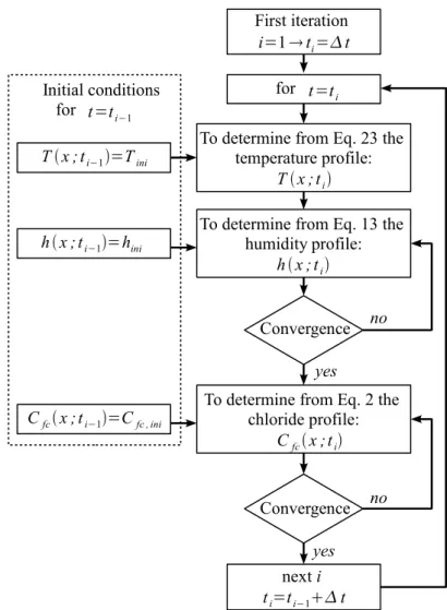
Figure 1 depicts the algorithm used to determine the time-dependent variation of the profiles of temper-ature, humidity and chlorides for one dimension –e.g., x. For the first iteration (i = 1) the initial values of temperature, humidity and concentration of free chlorides can be supposed as constants for all points inside the mesh –e.g. Tini, hini and Cf c,ini. Commonly the concentration of free chloride is set at zero at the beginning of the assessment. However, a given profile of chlorides can be used for existing structures. Thus, the algorithm to determine the profiles for a given time ti is summarized in the following steps:
1. the actual temperature profile is determined from Equation 23 by considering the initial temperature profile T (x; t = ti 1);
2. with the temperature profile estimated in the previous step T (x; t = ti) and the initial humidity profile h(x; t = ti 1), the actual humidity profile is determined from Equation 13; and finally;
3. Equation 2 is solved by accounting for the actual profiles of temperature and humidity throughout the concrete and the initial values of free chlorides Cf c(x; t = ti 1).
The procedure is repeated for the next i (ti = ti 1+ t) by considering the previous profiles as initial values. The major difficulty in estimating the profiles of humidity and chlorides lies in the fact that Equations
2 and 13 are nonlinear because the di↵usion coefficients and the isotherms depend on the actual profiles of humidity and chlorides; consequently, an iterative procedure is implemented. This procedure uses the profiles of h and Cf c obtained from the previous iteration, as the initial values and iterates until a given convergence criterion is reached. For example, for the profile of humidity in one dimension (i.e., x), the considered convergence criterion is:
h(x; ti)k+1 h(x; ti)k
h(x; ti)k " (27)
where k represents the iterations to find h(x; ti), h(x; ti)k is the humidity profile for the previous iteration, h(x; ti)k+1is the humidity profile for the actual iteration and " denotes a specified convergence parameter. A successive under-relaxation method is also implemented to increase the convergence rate. This method estimates a new humidity profile, h⇤(x; ti)k+1, that is used as initial value for the next iteration:
h⇤(x; ti)k+1= !h(x; ti)k+1+ (1 !)h(x; ti)k (28)
where ! is the relaxation factor varying between [0 1]. 3.3. Deterministic example
3.3.1. Problem description
The chloride penetration model allows introducing several mechanisms of ionic transfer in various en-vironmental conditions. The assessment of chloride ingress by considering both unsaturated media and time-dependent variation of temperature, humidity and surface chloride concentration, is illustrated in this section. Before performing a stochastic modeling, a deterministic analysis is needed to confirm that the results are physically compatible with underlying mechanisms and to analyze the sensitivity of the model to environmental actions. Towards this aim, the evolution of environmental parameters is modeled by deterministic functions which can be considered as mean trends. Thus, the following assumptions are made:
• the flow of chlorides occurs in one-dimension (e.g., concrete slab); • the structure is exposed to de-icing salts;
• the concrete is made with 400 kg/m3 of Ordinary Portland Cement (OPC) with 8% of C3A and water/cement ratio w/c = 0.5; and
• the concrete hydration time, te, is 28 days.
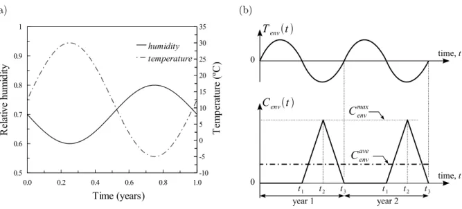
To account for seasonal variations of temperature and humidity, a sinusoidal variation is supposed: T (t) = max+ min 2 + max min 2 sin(2⇡t) (29) h(t) = max+ min 2 + max min 2 sin(2⇡(t 0.5)) (30)
where T (t) and h(t) are the temperature or humidity at time t, max is the maximum temperature or humidity, minis the minimum temperature or humidity and t is expressed in years. There exists correlation between temperature and humidity. In this work, this correlation is taken into account by considering that the water-vapor required to saturate air during cooler seasons is lower, and therefore, relative humidity is larger for these seasons. On the contrary, relative humidity has lower values for warmer seasons. Figure 2a shows the temperature and humidity models used in this example. The values of temperature and humidity,
, as well as the other constants used in the example are presented in Table 1.
In general, in chloride ingress modeling, it is assumed that the concentration of chlorides in the surround-ing environment remains constant for the exposure to de-icsurround-ing salts [29, 30]. However, since the kinematics of chloride ingress changes as function of weather conditions, a modified model for de-icing salts exposure is adopted in this work. This model considers that during the hot seasons the chloride concentration at the surface is zero, whereas during the cold seasons it becomes time-variant (Figure 2b):
Cenv(t) = 8 > > > < > > > : 0 for t < t1 Cmax env (t t1)/(t2 t1) for t1 t < t2 Cmax env [1 (t t2)/(t2 t1)] for t2 t < t3 (31) where Cmax
env is the maximum chloride concentration that corresponds with the minimum temperature and returns to zero at the beginning of the hot season (see Figure 2b). It is worthy to clarify that the value of Cmax
env has been defined by considering that the quantity of chloride ions deposited during one year be the same that the average annual concentration reported in the literature, Cave
env. For this example the value of Cmax
env presented in Table 1 entails that Cenvave= 4 kg/m3 [29, 30]. 3.3.2. Influence of environmental variations on chloride penetration
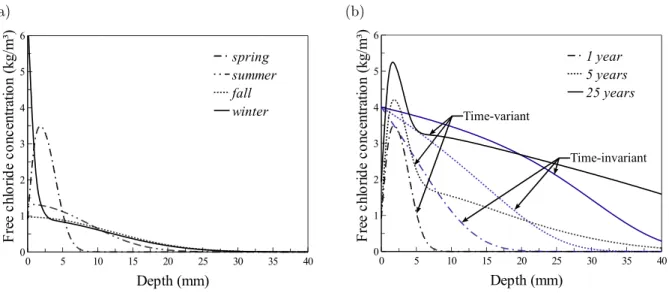
Figure 3a depicts the profiles of chlorides for di↵erent seasons after one year of exposure. The analysis begins at the end of exposure to chlorides (middle of spring) and ends when Cenv(t) is maximum (middle of winter). It should be noted that although de-icing salts are not applied during spring, summer and fall, the penetration front advances towards the reinforcement. Chloride ingress is more appreciable from spring to summer than from summer to fall because chloride di↵usivity increases for higher temperatures and humidities (see Equations 10 and 12). It can also be observed that during winter the chloride concentration tends to Cmax
env at the exposed surface.
Given that the shape of the chloride profiles depends on the season, Figure 3b presents the profiles after 1, 5 and 25 years of exposure at the middle of spring. These profiles were calculated for two types of environmental actions: time-variant and time-invariant. For the former the temperature and humidity are estimated from Equations 29 and 30 and the surface chloride concentration form Equation 31. In the latter, all the environmental variables are considered as constants –i.e., Cave
env= 4 kg/m3, Tenv= 12.5oC and henv = 0.7. For both cases, note that there is a large increase in the penetration depth from 1 to 5 years.
Nevertheless, the rate of chloride ingress decreases from 5 to 25 years. This reduction is due mainly to the decrease of chloride di↵usivity with time –i.e., Equation 11. If the cover thickness, ct, is 4 cm, it is also observed that for exposures higher than 5 yr the time-variant model gives greater concentration at ct. This result is due to the acceleration of chloride penetration during hot and wet seasons. This analysis confirms that transfer mechanisms are very sensitive to environmental actions. Therefore, it is needed to model these actions as realistic as possible. Given that probabilistic methods can be used to take into account their randomness, the next section presents a stochastic approach to improve the previous representation. 3.3.3. Comparison with the analytical error-function solution
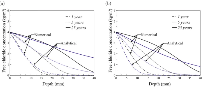
The most commonly used equation to model chloride penetration in concrete is the so-called “error-function solution” to Fick’s second law [1]. However, this analytical solution is not valid neither for curve-fitting exposure data nor for predictions because the di↵usivity and the surface chloride content are both time-dependent [31, 32]. Since this solution is still largely used, this section compares the results obtained with the proposed numerical approach with the results coming from the analytical error-function solution. To simplify the analysis, the inputs for temperature, humidity and surface chloride concentration are similar to those defined for the time-invariant case previously described (i.e., constant). Given that there is no experimental data to compute equivalent parameters for the analytical model, they have been computed from chloride profiles coming from the numerical model. The error function solution has two main governing parameters namely the surface chloride concentration and the chloride di↵usion coefficient. Since the surface chloride concentration is supposed to be constant for both models –i.e., Cave
env = 4 kg/m3, the problem is reduced to estimate the chloride di↵usion coefficient. This parameter is therefore found by minimizing the di↵erence between the data coming from analytical and numerical solutions.
The analytical model uses a time-invariant chloride di↵usion coefficient. Then, a chloride di↵usion co-efficient could be determined from each chloride profile. For instance, for the chloride profiles presented in Figure 3b and the time-invariant case, the chloride di↵usion coefficients for the analytical model are: 1.46⇥10 12 m2/s, 9.25⇥10 13 m2/s and 6.26⇥10 13 m2/s for 1, 5 and 25 years, respectively. It is noted that the instantaneous chloride di↵usion coefficient is time-variant and decreases with time. This study com-pares the chloride profiles computed from the numerical and the analytical models. Two chloride di↵usion coefficients were considered in the profiles coming from the analytical model. These di↵usion coefficients were obtained from the numerical results at 1 and 25 years. Figure 4 presents the chloride profiles estimated in both cases. It is noted in Figure 4a that analytical and numerical results are closer for 1 yr. In the second case (Figure 4b), it is observed that the analytical solution tends to average the numerical solution for 25 years. However, the shape of the error-function solution is very di↵erent from the shape of the numerical solution. These di↵erences emphasize the importance of including other phenomena in the calculation –i.e., chloride binding, a time-dependent chloride di↵usion coefficient, etc. Besides, these results show that the
analytical solution is very sensitive to the data used to determine the chloride di↵usion coefficient, and consequently, can over- or under-estimate the service life. Therefore, the lifetime assessment based on the error function solution of Fick’s law should be used with care.
4. Probabilistic analysis of chloride penetration
There is significant uncertainty related to environmental conditions, material properties, cover and model parameters. Therefore, to give appropriate estimations of chloride ingress into concrete, the model described in section 2 is introduced into a stochastic framework. The probabilistic approach proposed in this paper does not include spatial modeling of the uncertainties. Although spatial variability has been recognized as an influencing issue for probabilistic lifetime assessment of corroding RC structures [33], this section focuses on the determination of time-invariant and time-variant probabilistic models for chloride ingress. Stewart and Suo [34] present a comprehensive methodology to take spatial modeling of the uncertainties into account. 4.1. Probability of corrosion initiation
The corrosion initiation time, tini, is defined as the instant at which the chloride concentration at the cover reaches a threshold value, Cth. This threshold concentration represents the chloride concentration for which the rust passive layer of steel is destroyed and the corrosion reaction begins. Note that this threshold is sensitive to the chemical characteristics of concrete components: sand, gravel, cement. Consequently, it is assumed in this paper that Cthis a random variable. Time to corrosion initiation is obtained by evaluating the time-dependent variation of the chloride concentration in the cover depth by using the solution of the PDEs presented in section 3. The cumulative distribution function (CDF) of time to corrosion initiation, Ftini(t), is defined as:
Ftini(t) = P {tini t} = Z tinit f (x ¯) dx¯ (32) where x
¯ is the vector of the random variables to be taken into account and f (x¯) is the joint probability density function of x
¯. The limit state function becomes: g (x
¯,t) = Cth(x¯) Ctc(x¯,t, ct) (33)
where Ctc(x
¯,t, ct) is the total concentration of chlorides at the depth ctand the time t and ctis the thickness of the concrete cover. The failure probability, pf, represents, in this case, the probability of corrosion initiation and is obtained by integrating the joint probability function on the failure domain:
pf = Z g(x ¯,t)0 f (x ¯) dx¯ (34)
Given the complexity of the solution procedure used to estimate the time-dependent evolution of chloride profiles (section 3), closed-form solutions for both the CDF of time to corrosion initiation and probability
of corrosion initiation are impossible. Therefore, an appropriate tool to deal with this kind of problem is to use Monte Carlo simulations. This study also implements Latin Hypercube sampling to reduce the com-putational cost of simulations. For the adopted probabilistic approach, the random variables are classified into two groups: time-invariant and time-variant. The first group of variables depends on both the mate-rial properties and the construction procedure. Therefore, it can be assumed that time-invariant random variables remain constant during one Monte Carlo simulation. The material properties, cover thickness, and model parameters are included among these variables. The second group encompasses random variables changing during the period of analysis. Relative humidity, temperature and chloride concentration in the surrounding environment are considered as time-variant random variables and are modeled by stochastic processes as described in the following sections.
4.2. Stochastic modeling of weather: humidity and temperature
In order to make a good estimation of the time to corrosion initiation, it is important to implement a model that realistically reproduces the temperature and the humidity during the period of analysis. In this context, stochastic processes were used to model the random nature of these weather parameters. According to Ghanem and Spanos [27], there are two rational methods to deal with the problem under the probabilistic scheme: Karhunen-Lo`eve expansion or polynomial chaos. Taking into account the simplicity of the implementation and the computational time, Karhunen-Lo`eve expansion is appropriate to represent the weather variables.
4.2.1. Karhunen-Lo`eve expansion
Analogous to Fourier series, the Karhunen-Lo`eve expansion represents a stochastic process as a combi-nation of orthogonal functions on a bounded interval –i.e. [ a, a]. The development of a stochastic process by the Karhunen-Lo`eve method is based on the spectral decomposition of the covariance function of the process C(t1, t2). Since the covariance function is symmetric and positive definite, its eigenfunctions are orthogonal and form a complete set of deterministic orthogonal functions, fi(t), which are used to represent the stochastic process. The random coefficients of the process ⇠i(✓) can also be considered orthogonal or, in other words, statistically uncorrelated. Let (t, ✓) be a random process, which is function of the time t defined over the domain D, with ✓ belonging to the space of random events ⌦, (t, ✓) can thus be expanded as follows [27]: (t, ✓)' ¯(t) + nXKL i=1 p i⇠i(✓)fi(t) (35)
where ¯(t) is the mean of the process, ⇠i(✓) is a set of normal random variables, nKL is the number of terms of the truncated discretization and i are the eigenvalues of the covariance function C(t1, t2) resulting from
the evaluation of the following expression: Z
D
C(t1, t2)fi(t2)dt2= ifi(t1) (36)
The solution of Equation 36 can be analytically determined when the covariance function is exponential or triangular. In this work it is assumed that the processes of temperature and humidity have an exponential covariance of the form:
C(t1, t2) = e |t1 t2|/b (37)
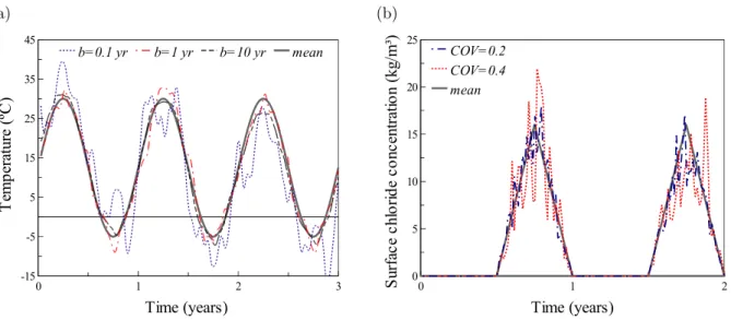
where b is the correlation length and must be expressed in the same units of t. For this case, the expressions to compute fi(t) and i are presented in detail in [27]. Finally, the mean of the stochastic process, ¯(t), is modeled as a sinusoidal function which considers the e↵ect of seasonal variations of the weather parameters –i.e., Equations 29 and 30. An advantage of this approach is that both the covariance function and the correlation length of weather parameters can be determined based on real measurements. Figure 5a shows some realizations of the stochastic process representing temperature where the parameters for the time-variant mean are described in Table 1. The considered correlation lengths are 0.1, 1 and 10 years; and the truncated discretization includes 30 terms (nLK = 30). Note that for lower values of b the process is far from the mean and extreme values are frequently observed.
4.3. Stochastic modeling of surface chloride concentration
The model described in this subsection is used to represent the surface chloride concentration produced by de-icing salts application. Due to lack of data about the variation of Cenvduring the exposure time and that various studies indicate that Cenv has a log-normal distribution [29, 30], the stochastic process representing Cenv is generated with independent log-normal numbers (log-normal noise). The mean of Cenv is described by Equation 31 and the COV used to generate the process is defined based on previous probabilistic studies [29, 30]. Stochastic representations of the surface chloride concentration are presented in Figure 5b. This figure considers a maximum surface chloride concentration, Cmax
env , equal to 16 kg/m3 and COVs of 0.2 and 0.4. As expected, the variability of the stochastic process increases for high values of COV.
5. Illustrative example
5.1. Problem description and basic assumptions
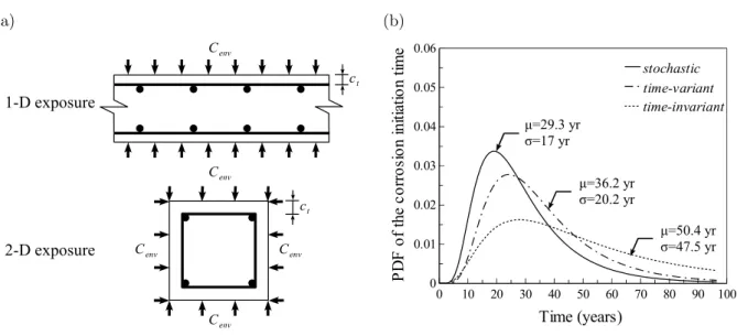
The main goal for this example is to study the influence of chloride binding, weather conditions, concrete aging, convection, correlation length and two-dimensional chloride ingress on the probability of corrosion initiation. Figure 6a shows the studied RC wall and column. It can be noted that chlorides come from one
direction for the one-dimensional exposure; whilst there is a source of chlorides in each side for the two-dimensional exposure. It is assumed herein that the structure is located well away from the seashore. Then, chlorides only come from de-icing salts. The weather features are presented in Table 1 and the probabilistic models used in this study are shown in Table 2.
The statistical parameters of the threshold concentration are defined based on the values reported in [30], where Cth is defined as the critical chloride content which leads to deterioration or damage of the concrete structure when the structure is constantly humid. The cover thickness, ct, follows a truncated normal distribution with the statistical parameters indicated in Table 2 [29, 30]. The means of the reference di↵usion coefficients of humidity and chlorides, Dh,ref and Dc,ref, are assigned according to the experimental values presented in [3] for w/c = 0.5. The probabilistic models and COVs of Dh,ref and Dc,ref, follow the distributions suggested in [9, 30]. Based on the sources presented in Table 1, it is supposed that ↵0, n, Uc, and cq follow beta distributions with the mean reported by the authors and varying between the limits established experimentally. The COVs of these variables were determined on the basis of the experimental results reported in Table 1. According to Val [22], the age reduction factor m also follows a beta distribution. Finally taking as a reference the typical density of normal concrete, it is assumed that this variable is normally distributed with a COV of 0.04 [35].
Other assumptions of this example are:
• the concentration of chlorides inside concrete is zero at the beginning of the analysis; • the finite di↵erence weighting factor is 0.8, and the relaxation factor is ! = 0.9; • the structure is located in a partially-saturated environment;
• the studied concrete contains 400 kg/m3 of Ordinary Portland Cement (OPC) with 8% of C3A and w/c = 0.5;
• the constants of the isotherms are ↵L= 0.1185, L = 0.09, ↵F = 0.256, F = 0.397 and were obtained for ordinary OPCs with the same characteristics [14, 15];
• the hydration period, te, is 28 days;
• the COV used to generate the stochastic process of Cenv is equal to 0.4;
• the range of each random variable is divided into 10 equally probable intervals for the Latin Hypercube sampling and
5.2. Results
The results of Monte Carlo simulations were adjusted to an appropriate PDF, where the test of Kolmogorov-Smirnov (K-S) with a significance level of 5% was used as selection criterion. For all the studied cases, and according to [36], the results indicate that the time to corrosion initiation is log-normally distributed.
Figure 6b depicts the influence of the type of weather model –i.e., time-invariant, time-variant and stochastic, on the PDF of the corrosion initiation time. For the time-invariant case the annual temperature and relative humidity were set to 12.5 C and 0.7, respectively. Such values correspond to the annual mean for the time-variant model. The time-variant case accounts for the sinusoidal variation of temperature and humidity described by Equations 29 and 30 and the values presented in Table 1. The stochastic case considers the stochastic model presented in subsection 4.2 where the mean is defined by the time-variant model and the correlation length is 0.1 year. It should be noted that the mean and standard deviation of the corrosion initiation time decrease when both the seasonal variations and the randomness of humidity and temperature are considered. Taking as a reference the mean obtained from the stochastic analysis, it is observed that the mean of the corrosion initiation time is increased by 23% and 94% for the time-variant and time-invariant models, respectively. This increase is expected because as showed in Figure 3b, accounting for the seasonal variation of humidity and temperature (time-variant model) reduces the corrosion initiation time. The reduction is more appreciable when the time-variant model is coupled with a stochastic process, for which there are extreme values that accelerate chloride penetration. Give that under real exposure the structure is subject to random environmental actions, these results highlight the importance of including comprehensive probabilistic models of weather actions in the chloride ingress assessment.
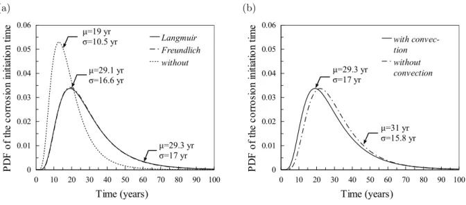
The e↵ect of chloride binding and the type of isotherm on the PDF of the corrosion initiation time is showed in Figure 7a. This analysis considers temperature and humidity as stochastic processes with a correlation length of 0.1 year. As expected, the results indicate that ignoring the e↵ect of chloride binding reduces the mean of the corrosion initiation time in comparison to the cases where this e↵ect was considered. This behavior seems reasonable because when binding is not considered, it is assumed that all the chlorides involved in the flow (bound and free) ingress simultaneously into the concrete matrix, and therefore, the time to corrosion initiation occurs early. By comparing the results for the Langmuir and Freundlich isotherms, it can be observed that there is no significant di↵erence for both models. This similarity lies in the fact that the constants for both isotherms were determined for concrete with identical characteristics. It allows to suggest that for this type of studies, no improvement in this direction is needed.
The impact of convection on the PDF of the corrosion initiation time is plotted in Figure 7b. These PDFs were obtained for the Langmuir isotherm, correlation length of 0.1 year, and by modeling environmental actions stochastically. It can be noted from Figure 7b that accounting for chloride ingress by convection slightly decreases the mean of the corrosion initiation time. This reduction is due to the addition of a second mechanism of chloride ingress (i.e., convection) which augments the chloride concentration at the corrosion
cell reducing the time to achieve the threshold concentration. In this example, the e↵ect of convection on chloride penetration is not very important because the structure is not subjected to cycles of wetting and drying. However, under other exposure conditions, wetting-drying cycles accelerate appreciably chloride penetration by carrying chloride ions with water.
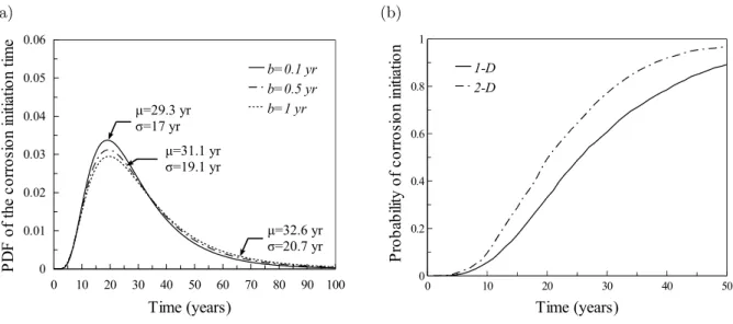
Figure 8a describes the influence of the correlation length b (i.e., Equation 37) on the probability of corrosion initiation. For this study correlation lengths of 0.1, 0.5 and 1 year, have been simply assumed. Although this value should be determined based on real measurements of temperature and humidity for a determined place, the results indicated that its influence on the mean and standard deviation of the probability of corrosion initiation is not important. Moreover, it is noticed that the smaller values of b lead to conservative results. This behavior is expected because smaller values of b entail the presence of extreme values (see Figure 5a) that accelerate the process of chloride ingress.
Finally, the variation of the probability of corrosion initiation for 1-D and 2-D exposures is showed in Figure 8b. Both cases include the probabilistic nature of environmental actions, chloride ingress by convection, chloride binding and a correlation length of 0.1 years. As expected the higher probabilities correspond to the 2-D exposure. The reduction of the corrosion initiation time is due to the exposure to chlorides on both sides of the structural element. For instance, for 30 years of exposure the probability of corrosion initiation is increased by 27% when 2-D exposure is considered. These results stress the importance of including a two-dimensional analysis for correct prediction of corrosion initiation in small RC elements as columns and beams.
6. Conclusions and further work
This paper presented a stochastic approach to assess chloride ingress into concrete considering the ef-fects of chloride binding, temperature, humidity, concrete aging and convection. The problems of chloride transport, moisture transport and heat transfer into concrete were treated by combining the finite element formulation with finite di↵erence. The model of chloride penetration was introduced in a stochastic frame-work where Monte Carlo simulations and Latin hypercube sampling were used to account for the randomness related to the phenomena. The proposed probabilistic approach distinguishes between two types of random variables ”time-invariant” and ”time variant”. The latter are treated as stochastic processes which are modeled by Karhunen-Lo`eve expansions and log-normal noise.
The proposed approach is illustrated by a numerical example where the factors controlling the chloride ingress and the e↵ect of weather conditions were studied. Overall behavior indicates that the mean of corrosion initiation time decreases when the randomness and seasonal variations of humidity, temperature and Cenv and convection are considered; and increases when chloride binding is taken into account. By comparing chloride penetration in one- and two-dimensions, it has been found that high probabilities of
corrosion initiation correspond to the 2-D exposure. These results stress the importance of including the e↵ects and the random nature of temperature, humidity, surface chloride concentration, chloride binding, convection and two-dimensional chloride ingress for a comprehensive lifetime assessment.
There are many areas in which further research is needed to improve the probabilistic model of chloride penetration. These improvements as summarized as follows:
• determination of model parameters for a wide range of concrete types;
• formulation and implementation of a model that considers the kinematics between concrete cracking and chloride penetration;
• study of the influence of hourly, daily and weekly variations of temperature and humidity on chloride ingress;
• assessment and consideration of the correlation of material properties and climatic conditions from experimental data;
• consideration of the spatial variability of the phenomenon; and
• characterization and modeling of error propagation in the whole deterioration process. Acknowledgments
The contribution of Mrs. Silvia Caro to the calibration of the finite element model is gratefully acknowl-edged by the authors. The authors acknowledge financial support of the project ’Maintenance and REpair of concrete coastal structures: risk-based Optimization’ (MAREO Project – contact: [email protected]).
References
[1] Tuutti K. Corrosion of steel in concrete. Swedish Cement and Concrete Institute 1982.
[2] Nilsson LO, Sandberg P, Poulsen E, Tang L, Andersen A, Frederiksen JM (1997). HETEK, a system for esti-mation of chloride ingress into concrete, Theoretical background. Danish Road Directorate Report, No. 83. [3] Saetta A, Scotta R, Vitaliani R. Analysis of chloride di↵usion into partially saturated concrete. ACI Mater J
1993;5:441–51.
[4] Ababneh AN, Benboudjema F, Xi Y. Chloride penetration in unsaturated concrete. J Mater Civ Eng ASCE 2003;15:183–91.
[5] Val DV, Stewart MG, Melchers RE. E↵ect of reinforcement corrosion on reliability of highway bridges. Eng Struct 1998;20:1010–19.
[6] Bastidas-Arteaga E, S´anchez-Silva M, Chateauneuf A, Ribas Silva M. Coupled reliability model of biodeterio-ration, chloride ingress and cracking for reinforced concrete structures. Struct Saf 2008;30:110–29.
[7] Bastidas-Arteaga E, Bressolette Ph, Chateauneuf A and S´anchez-Silva M. Probabilistic lifetime assessment of RC structures under coupled corrosion-fatigue processes. Struct Saf 2009;31:84–96.
[8] Kong JS, Ababneh AN, Frangopol DM, Xi Y. Reliability analysis of chloride penetration in saturated concrete. Probab Eng Mech 2002;17:305–15.
[9] Val DV, Trapper PA. Probabilistic evaluation of initiation time of chloride-induced corrosion. Reliab Eng Sys Safety 2008;93:364–72.
[10] Mart´ın-P´erez B, Pantazopoulou SJ, Thomas MDA. Numerical solution of mass transport equations in concrete structures. Comput Struct 2001;79:1251–64.
[11] Djerbi A, Bonnet S, Khelidj A, Baroghel-Bouny V. Influence of transversing crack on chloride di↵usion into concrete. Cem Concr Res 2008;38:877–83.
[12] Neville A. Chloride attack of reinforced concrete: an overview. Mater Struct 1995;28:63–70.
[13] Nilsson L-O, Massat M, Tang L. The e↵ect of non-linear chloride binding on the prediction of chloride penetration into concrete structures. In V. Malhotra (Ed.), Durability of Concrete, ACI SP–145. Detroit 1994. p. 469–86. [14] Tang L, Nilsson LO. Chloride binding capacity and binding isotherms of OPC pastes and mortars. Cement
Concr Res 1993;23:247—53.
[15] Glass G, Buenfeld N. The influence of the chloride binding on the chloride induced corrosion risk in reinforced concrete. Corros Sci 2000;42(2):329–44.
[16] Baˇzant Z, Najjar L. Drying of concrete as a nonlinear di↵usion problem. Cement Concr Res 1971;1:461–73. [17] Baˇzant Z, Najjar L. Nonlinear water di↵usion in nonsaturated concrete. Mater Struct 1972;5:3–20.
[18] Brunauer S, Skalny J, Bodor E. Adsorption on non-porous solids. J Colloid Interface Sci 1969;30:546–52. [19] Xi Y, Baˇzant Z, Jennings H. Moisture di↵usion in cementitious materials – Adsorption isotherms. Adv Cem
Based Mater 1994;1:248–57.
[20] Han SH. Influence of di↵usion coefficient on chloride ion penetration of concrete structures. Constr Build Mater 2007;21(2):370–8.
[21] Page C, Short N, Tarras AE. Di↵usion of chloride ions in hardened cement pastes. Cem and Concr Res 1981;11:395–406.
[22] Val DV. Service-life performance of RC structures made with supplementary cementitious materials in chloride-contaminated environments. In: Proceedings of the international RILEM-JCI seminar on concrete durability and service life planning, Ein-Bokek, Israel, 2006. p. 363–73.
[23] Baˇzant Z, Thonguthai W. Pore pressure and drying of concrete at high temperature. J Eng Mech Div 1978;(104):1059–1079.
[24] Akita H, Fujiwara T, Ozaka Y. A practical procedure for the analysis of moisture transfer within concrete due to drying. Mag Concr Res 1997;49:129–37.
[25] Neville A. Properties of Concrete. 3rd ed. Longman Scientific & Technical; 1981.
[26] Khan A, Cook W, Mitchell D. Thermal properties and transient thermal analysis of structural members during hydration. ACI Mat J 1998;95:293–303.
[27] Ghanem RG, Spanos PD. Stochastic Finite Elements: A Spectral Approach. Springer New York, USA; 1991. [28] McGee R. Modelling of durability performance of Tasmanian bridges. In: Melchers RE, Stewart MG, editors.
Applications of statistics and probability in civil engineering. Rotterdam: Balkema; 2000. p. 297–306.
[29] Vu KAT, Stewart MG. Structural reliability of concrete bridges including improved chloride-induced corrosion models. Struct Saf 2000;22:313–33.
[30] DuraCrete. Probabilistic performance based durability design of concrete structures. The European Union–Brite EuRam III; 2000.
[31] Luping T, Gulikers J. On the mathematics of time-dependent apparent chloride di↵usion coefficient in concrete. Cem Concr Res 2007;37:589–95.
[32] Nilsson LO, Frederiksen JM. On uncertainties and inaccuracies in empirical chloride ingress modeling. In: Ait-Moktar K, Breysse D, editors. Marine Environmental Damage to Atlantic Coastal and Historical Structures, MEDACHS’10. La Rochelle, France; 2010. p. 3–10.
[33] Stewart MG, Mullard JA. Spatial time-dependent reliability analysis of corrosion damage and the timing of first repair for RC structures. Eng Struct 2007;29:1457–64.
[34] Stewart MG, Suo Q. Extent of spatially variable corrosion damage as an indicator of strength and time-dependent reliability of RC beams. Eng Struct 2009;31:198–207.
[35] Joint Committee of Structural Safety. Probabilistic Model Code, Internet Publication: www.jcss.ethz.ch; 2001. [36] Lounis Z. Uncertainty modeling of chloride contamination and corrosion of concrete bridges. In: Attoh-Okine NO, Ayyub BM editors. Applied research in uncertainty modeling and analysis. USA: Springer;2005. p. 491–511.
List of Tables
• Table 1. Values used in the deterministic example. • Table 2. Probabilistic models of the random variables.
List of Figures
• Fig. 1. Algorithm for estimating the profiles of temperature, humidity and chlorides.
• Fig. 2. (a) Temperature and humidity models. (b) Environmental chloride surface concentration. • Fig. 3. Profiles of Cf c for (a) di↵erent seasons after one year of exposure and (b) the middle of spring
and various times of exposure.
• Fig. 4. Chloride profiles for the analytical model and the numerical solution for di↵usion coefficients estimated at (a) 1 year and (b) 25 years.
• Fig. 5. Realizations of (a) temperature and (b) surface chloride concentration.
• Fig. 6. (a) Cross-sections of the studied RC wall and column. (b) Impact of weather model. • Fig. 7. E↵ect of (a) binding and type of isotherm and (b) convection.
• Fig. 8. (a) Influence of the correlation length b. (b) Probability of corrosion initiation for 1-D and 2-D exposures.
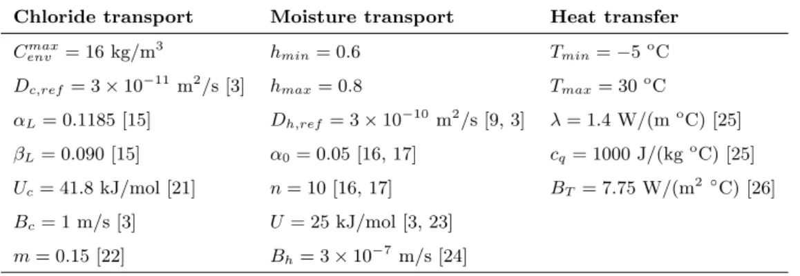
Table 1: Values used in the deterministic example.
Chloride transport Moisture transport Heat transfer
Cenvmax= 16 kg/m3 hmin= 0.6 Tmin= 5oC
Dc,ref= 3⇥ 10 11m2/s [3] hmax= 0.8 Tmax= 30oC
↵L= 0.1185 [15] Dh,ref= 3⇥ 10 10m2/s [9, 3] = 1.4 W/(moC) [25] L= 0.090 [15] ↵0= 0.05 [16, 17] cq= 1000 J/(kgoC) [25] Uc= 41.8 kJ/mol [21] n = 10 [16, 17] BT= 7.75 W/(m2 C) [26] Bc= 1 m/s [3] U = 25 kJ/mol [3, 23] m = 0.15 [22] Bh= 3⇥ 10 7m/s [24] 22
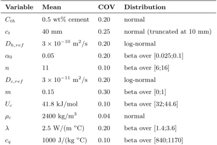
Table 2: Probabilistic models of the random variables.
Variable Mean COV Distribution
Cth 0.5 wt% cement 0.20 normal ct 40 mm 0.25 normal (truncated at 10 mm) Dh,ref 3⇥ 10 10 m2/s 0.20 log-normal ↵0 0.05 0.20 beta over [0.025;0.1] n 11 0.10 beta over [6;16] Dc,ref 3⇥ 10 11 m2/s 0.20 log-normal m 0.15 0.30 beta over [0;1]
Uc 41.8 kJ/mol 0.10 beta over [32;44.6]
⇢c 2400 kg/m3 0.04 normal
2.5 W/(moC) 0.20 beta over [1.4;3.6] cq 1000 J/(kgoC) 0.10 beta over [840;1170]
Cfc x ;ti−1=Cfc , ini Initial conditions for t=ti−1 T x ;ti−1=Tini h x ;ti−1=hini First iteration i=1 ti=t for t=ti
To determine from Eq. 23 the temperature profile:
T x ;ti
To determine from Eq. 13 the humidity profile:
h x ;ti
To determine from Eq. 2 the chloride profile: Cfc x ;ti Convergence next i ti=ti−1 t yes no yes no Convergence
Figure 1: Algorithm for estimating the profiles of temperature, humidity and chlorides.
(a) (b) 0.0 0.2 0.4 0.6 0.8 1.0 0.5 0.6 0.7 0.8 0.9 1 -10 -5 0 5 10 15 20 25 30 35 humidity temperature Time (years) R el at iv e hu m id ity T em pe ra tu re ( ºC ) year 1 year 2 t1 t2 t3 t1 t2 t3 time, t time, t 0 0
C
envt
T
envt
C
envmaxC
envave(a) (b) 0 5 10 15 20 25 30 35 40 0 1 2 3 4 5 6 spring summer fall winter Depth (mm) Fr ee c hl or id e co nc en tr at io n (k g/ m ³) 0 5 10 15 20 25 30 35 40 0 1 2 3 4 5 6 1 year 5 years 25 years 1 year 5 years 25 years Depth (mm) Fr ee c hl or id e co nc en tr at io n (k g/ m ³) Time-variant Time-invariant
Figure 3: Profiles of Cf cfor (a) di↵erent seasons after one year of exposure and (b) the middle of spring and various times of exposure.
(a) (b) 0 5 10 15 20 25 30 35 40 0 1 2 3 4 5 6 1 year 5 years 25 years 1 year 5 years 25 years Depth (mm) Fr ee c hl or id e co nc en tr at io n (k g/ m ³) Numerical Analytical 0 5 10 15 20 25 30 35 40 0 1 2 3 4 5 6 1 year 5 years 25 years 1 year 5 years 25 years Depth (mm) Fr ee c hl or id e co nc en tr at io n (k g/ m ³) Numerical Analytical
Figure 4: Chloride profiles for the analytical model and the numerical solution for di↵usion coefficients estimated at (a) 1 year and (b) 25 years.
(a) (b) 0 1 2 3 -15 -5 5 15 25 35 45 b=0.1 yr b=1 yr b=10 yr mean Time (years) Te m pe ra tu re ( ºC ) 0 1 2 0 5 10 15 20 25 COV=0.2 COV=0.4 mean Time (years) Su rf ac e ch lo rid e co nc en tr at io n (k g/ m ³)
Figure 5: Realizations of (a) temperature and (b) surface chloride concentration.
(a) (b) ct ct Cenv Cenv Cenv Cenv Cenv 1-D exposure 2-D exposure 0 10 20 30 40 50 60 70 80 90 100 0 0.01 0.02 0.03 0.04 0.05 0.06 stochastic time-variant constant Time (years) PD F of th e co rr os io n in iti at io n tim e μ=29.3 yr σ=17 yr μ=36.2 yr σ=20.2 yr time-invariant μ=50.4 yr σ=47.5 yr
(a) (b) 0 10 20 30 40 50 60 70 80 90 100 0 0.01 0.02 0.03 0.04 0.05 0.06 Langmuir Freundlich without Time (years) P D F o f th e co rr os io n in iti at io n tim e μ=29.1 yr σ=16.6 yr μ=19 yr σ=10.5 yr μ=29.3 yr σ=17 yr 0 10 20 30 40 50 60 70 80 90 100 0 0.01 0.02 0.03 0.04 0.05 0.06 with convec-tion without convection Time (years) P D F o f th e co rr os io n in iti at io n tim e μ=29.3 yr σ=17 yr μ=31 yr σ=15.8 yr
Figure 7: E↵ect of (a) binding and type of isotherm and (b) convection.
(a) (b) 0 10 20 30 40 50 60 70 80 90 100 0 0.01 0.02 0.03 0.04 0.05 0.06 b=0.1 yr b=0.5 yr b=1 yr Time (years) P D F o f th e co rr os io n in iti at io n tim e μ=29.3 yr σ=17 yr μ=31.1 yr σ=19.1 yr μ=32.6 yr σ=20.7 yr 0 10 20 30 40 50 0 0.2 0.4 0.6 0.8 1 1-D 2-D Time (years) Pr ob ab ili ty o f co rr os io n in iti at io n