CIRPÉE
Centre interuniversitaire sur le risque, les politiques économiques et l’emploi
Cahier de recherche/Working Paper 06-38
Poverty and Inequality Nexus: Illustrations with Nigerian Data
Abdelkrim Araar
Awoyemi Taiwo Timothy
Novembre/November 2006
___________________
Araar: Département d’économique and CIRPÉE, Pavillon J.-A.-DeSève, Université Laval, Québec QC Canada G1K 7P4 / Fax: 1-418-656-7798
Taiwo: Department of Economics, University of Ibadan, Nigeria / Fax: 1-418-656-7798 [email protected]
Abstract:
The main aim of this paper is to explore the link between poverty and inequality. In developing countries, there is a general consensus that high inequality can dampen significantly the impact of economic performance on poverty. In this paper, we propose a new theoretical framework that links poverty and inequality. We also show between and within group inequalities, as well as inequality in income sources, can contribute to total poverty. The methodology of the paper is illustrated using the 2004 Nigerian national living standard survey.
Keywords: Poverty, Inequality JEL Classification: D 6 3 , D 6 4
1 Introduction
There has been a recent upsurge of interest among both policy makers and researchers in the link between poverty and inequality in their static and dynamic forms. Indeed, understanding the contribution of total inequality or its compo-nents to total poverty can help design appropriate economic policies to reduce in-equality and poverty. The aim of this paper is to propose a new theoretical frame-work to establish a link between poverty and inequality. Among other things, we decompose the value of poverty indices into contributions of average income and various inequality components.
The usual main components of inequality that are modelled in the literature are the between-groups, the within-groups and income-sources inequalities. To perform a decomposition of total poverty into contributions of such a set of com-ponents, we use the Shapley approach1. An application of this approach to
de-compose distributive indices was recently introduced by Shorrocks (1999). A nice property of such an approach is the additivity of the contribution of components and the exactness of the decomposition, by which the residue due to the interac-tion between components is attributed to each of the components by means of a linear approximation.
While there is a growing consensus concerning the links between average in-come, inequality and poverty in a static setting, the dynamic link and its optimal path raise another set of issues. Indeed, this “socially” optimal path can shape the temporal governmental interventions in terms of redistribution or investment in the human capital or in the basic infrastructures. Kuznets (1956) indicates that the link between growth in GDP per capita and inequality should take an inverse U shape during economic development. Empirical studies have tended to show that such a U shape cannot be observed for many countries. To assess the contri-bution of growth and redistricontri-bution to the evolution of poverty, Datt and Ravallion (1992) decompose the observed variation in poverty into growth and redistribution components. A technical improvement to this method was proposed by Kakwani (1997) and Shorrocks (1999). Even if the decomposition proposed in this paper is static, its application in a dynamic setting is straightforward since this decompo-sition can be used to explain the observed variation in total poverty by variations in the contribution of components.
The plan of this paper is as follows. In the next section, we review the static and dynamic links between poverty and inequality. In the third section, we
form the decomposition of total poverty into components of average income and between and within groups inequalities. In the fourth section, we decompose total poverty into average-income and inequality-in-income-sources components. In section five, we illustrate the methodology using the 2004 Nigerian living stan-dard survey. Finally, some concluding remarks are made in section six.
2 The Link Between Poverty and Inequality
This section reviews the link between poverty and inequality under both static and dynamic settings.
2.1 The static link between poverty and inequality
Under a static setting, the two main components of poverty are the average standard of living and shape of the relative distribution (or inequality). An in-crease in average income is linked negatively with poverty whereas an inin-crease in inequality increases poverty. The temporal evolution of these two components, that are growth and redistribution components, determines the observed variation in poverty. What can be the link between the evolution of these two components and poverty? We try to answer this question in the following subsection.
2.2 The dynamic link between poverty and inequality
Kuznets (1956) suggests that the link between economic growth, represented by the growth in GDP per capita, and inequality takes an inverted U shape dur-ing the development period of a country. This postulate is based on the steps of development that he posited:
I: The primary sector (agriculture) represents the main part in the structure of the economic activity. This phase is characterized by a quasi uniform distribution of income and a low level of inequality.
II: The emergence of the secondary sector (industry) with higher level of pro-ductivity compared to the primary sector. This implies an increase in between-group inequality as well as in total inequality.
III: Introduction of new technologies in the primary sector partly eliminates the difference in productivity and incomes. Therefore, total inequality is reduced.
The experience during the last few decades shows that the tertiary sector repre-sents an important part of a country’s economy. In the last two decades, many researchers have found little signs of a systematic relationship between growth and inequality 2. However, the main aim of Kuznets theory on the link between
disparities in the productivity of economic sectors and inequality continues to be relevant even if the complete U shape cannot be observed empirically for many countries3. The ambiguity concerning the link between growth and inequality can
be explained by the lower correlation between them. Inequality is linked to the disparity in the productivity of economic sectors rather than economic growth. This disparity can be higher in economic crisis or economic expansion periods. During recession periods, some sectors are more affected by economic shocks than others. This can explain the increase in inequality in developing countries even if the economic growth rate decreases. During expansion periods however, some economic sectors perform better than others. This boosts economic growth but worsens the income distribution.
Datt and Ravallion (1992) decompose the observed variation in poverty into growth and redistribution. This method was improved by Kakwani (1997) and Shorrocks (1999) to deal with the non attributed residue. While the Datt and Ravallion approach explores how the growth in average income affects total poverty, earlier work on pro-poor growth focuses more on the nature of this impact at dif-ferent segments of the distribution4.
2.3 Poverty indices and inequality
As mentioned earlier, average income and the level of inequality are the two factors that determine the level of poverty. When incomes are equally distributed, poverty indices depend on the difference between the poverty line and the average income. Generally, poverty indices can be decomposed as follows:
P (y, z) = Eµ+ Eπ (1)
2For this, seeDeininger and Squire (1998), Fields (1989) and Ravallion and Chen (1997). 3Deininger and Squire (1998) uses data set of higher quality containing 682 observations on the
Gini index for 108 countries. These authors conclude that there exists no support for the Kuznets hypothesis of inverted U-shaped curve. When tested on a country-by-country basis, they found that 90 percent of the countries investigated did not validate the Kuznets hypothesis.
4See Ravallion and Datt (2002), Ravallion and Chen (2003), Kakwani, Khandker, and Son
where y represents the vector of incomes, z is the poverty line, Eµ is the
contri-bution of average income (µ) with perfect equality and Eπ is the contribution of
total inequality (π) with the observed average income. Formally, we can re-write the contribution of average income as:
Eµ|π=0 =
½
0, when µ ≥ z
P (µ, z), when µ < z. (2)
Equation (2) indicates that the quasi perfect equality is not sufficient to eliminate poverty when the average income is very low. In the case when average income is close to the poverty line, any rise in inequality implies a significant increase in poverty. In the other case when average income is relatively high (in developed countries for example), one can observe that the best economic performance pe-riods were accomplished frequently by an increase in inequality. Moreover, this situation can also be Pareto optimal in a dynamic way, where the wellbeing of each household is improved or at the limit, does not worsen5.
One can note that, even if poverty indices are not sensitive to inequality within the poor group, like the headcount and poverty gap indices, they continue to be sensitive to the inequality between the poor and non poor groups. In addition, one can note that, with the focus axiom that most poverty indices obey, they are not sensitive to the inequality within the non poor group.
2.4 Gini index Lorenz curve and poverty
The Lorenz curve is a useful tool to represent the overall inequality. As shown by Datt and Ravallion (1992), the link between the headcount, noted by H, and the Lorenz curve is:
L0(H) = z
µ (3)
The link between the average poverty gap, denoted by P 1, and inequality repre-sented by the Lorenz curve is:
P 1 = [z − µp] H (4)
where µp is the average income of the poor group. The link between the severity
index, represented by the square of the poverty gaps and the Lorenz curve can be written as: P 2 = Z H 0 [z − µL0(p)]2dp (5) 5See Feldstein (1998).
One of the most popular inequality indices is the Gini index. Since the group-income overlap does not exist between the poor and non poor group, the Gini index is easily decomposable across poor and non-poor groups and the residue due to the overlap equals to zero6. This decomposition takes the following form:
I = φpψpIp+ φnpψnpInp+ ˜I (6)
where I is the Gini index, φg and ψg are the population and income shares for
the group g respectively and ˜I is the Gini index where within group inequality is
eliminated, i.e., each household has the average income of its group. Based on this, the link between headcount index and the between group inequality is7:
H = µ ˜I µ 1 µ − µp ¶ (7) Starting from the last equation, we find that the component between group in-equality can be expressed as follows:
˜
I = H − L(H) (8)
where L(H) is the level of the Lorenz curve when the percentile p = H. Thus, the between inequality, measured by the Gini index, equals to the deficit share of the poor group. More this deficit is lower, more is lower the inequality between the poor and the non poor groups. For the poverty gap index, the link can be expressed as8: P 1 = µ ˜I µ z − µp µ − µp ¶ (9) The link between the Gini index and severity indices of poverty cannot be estab-lished directly. This is explained by the different shapes that the distribution can have, with the same level of inequality measured by Gini index.
3 Population Groups, Inequality and Poverty
In this section, we show how the between and the within group inequalities contribute to the total poverty. This is an important investigation as it provides answers to the following questions:
6See Lamber and Aronson (1993) and Araar (2006) 7See the prove in appendix A.
8Recall that P 1 = H(z − µ
• What is the contribution of regional disparities to the total poverty?
• What is the contribution of the within group inequality of a given group (urban area for example) to total poverty?
The form of decomposition, that we propose to answer these questions, takes the following form: P (y, z) = Eµ+ EB+ G X g=1 EWg (10)
where EBis the contribution of the between group inequality and EWg is the
con-tribution of inequality within the group g.
By the term “marginal contribution” of a component, we refer to the variation in poverty index generated by removing such component. To estimate, at the margin, the contribution of the within group inequality to the total poverty, we compare between poverty index with the observed household incomes and that would occur if the within group inequality is removed. For this, we use a vector of income where each household has the average income of its group, noted by
µg. Formally, we have that:
MW = P (y) − P (µg) (11)
To eliminate the intergroup inequality and to estimate the contribution at the mar-gin of the intragroup inequality to total poverty, we will use a vector of income where each household is given its income scaled by the ratio µ/µg. With this new
income vector, the average income of each group equals to µ.
MB = P (y) − P (y.µ/µg) (12)
Even if this procedure gives us an idea on the contribution of each factor, this approach overestimate their contributions such that:
Eπ < MW + MB (13)
To avoid this drawback, we use the Shapley approach, by keeping the same rules for eliminating each of the between and within group factors9.
Eπ = EW + EB (14)
where
EB = 0.5 [P (y) − P (y(µ/µg)) + P (µg) − P (µ)] (15) EW = 0.5 [P (y) − P (µg) + P (y(µ/µg)) − P (µ)] (16)
For the additive class of poverty indices, the within group contribution can be easily decomposed across groups as follows:
EW = G X g=1 EWg (17) such that: EWg = 0.5φg[Pg(y) − Pg(y(µ/µg)) + Pg(µg) − Pg(µ)] (18)
where φg is the population share of group g. If poverty index is not additively
separable in population groups, one can perform a second stage decomposition, with the Shapley approach, analogously to what was proposed in Araar (2006) for the decomposition of the Gini index.
4 Inequalities in Income Sources and Poverty
It is also interesting to estimate the contributions of inequalities in income sources to total poverty. First, we assume that the sum of K income sources equals the total income and the amount of income source k, is denoted by sk. The
contribution of the inequality of income source k at the margin, is the difference between the observed total poverty and that when the inequality of this component is eliminated. Formally, we replace skby µkfor each household if the component k is eliminated.
Mk = Eπ − P (y∗ =
X
j
sj6=k + µk) (19)
Here we find that:
Eπ <
X
k
Mk (20)
for this, we suggest to use the Shapley approach with the same rule for removing inequalities in income sources.
5 Illustration Using Nigeria National Survey
The survey data used in this study was collected by Nigeria’s National Bu-reau of Statistics (NBS) formerly known as the Federal Office of Statistics (FOS). They were based on National Living Standard Survey (NLSS) of households that was carried out between September 2003 and August 2004. The sample design is a two-stage stratified sampling. At the first stage, clusters of 120 housing units called Enumeration Area (EA) were randomly selected from each State and the Federal Capital Territory (FCT, Abuja). The second stage involved random selec-tion of 5 housing units from the selected EAs. A total of 600 households were randomly chosen in each of the States and the FCT, summing up to 22,200 house-holds in all (FOS, 2003). However, some househouse-holds did not fully complete the questionnaires. Out of the 22,200 households that were targeted, only 19,158 completed the survey.
In this application, two main standard of living are adopted. The first is the total expenditure per capita and the second is the per capita income. The latter is useful to perform the decomposition of poverty by components of inequalities in income sources. It should be noted that there is no official absolute poverty line in Nigeria. Usually, the relative approach is adopted to estimate the poverty line in Nigerian studies (poverty line equals to two third of average standard of living). In this study, we additionally use the World Bank poverty line, that is US$1 per day by adult equivalent.
In this application, we analyse the contribution of the regional disparities (be-tween group inequality) and inequality within each of the six geopolitical zones to the total inequality and poverty10. Moreover, we estimate the contribution of
the observed inequalities in income sources to total inequality and poverty. Figure (1), illustrates the density curves for the six geopolitical zones in Nige-ria. It is obvious from the comparisons between density curves, that the north east and north center are the poorest zones. Furthermore, the well-being of households living in south east and south west is better than the well-being of the other house-holds. Similarly, these conclusions are confirmed by comparing between FGT curves (α = 0), as presented in figure (2). In table (1), we decompose the FGT index by the six zones. Results of this decomposition indicate that more than 64% of total poverty is attributed to the population group that live in northern zones, while this group represents about 53% of total population.
Figure 3 shows clearly how the poor and the non poor groups, as well as, the
interaction between them contribute to the total inequality, measured by the Gini index (review again equation (6)). The contribution of the within poor group to the total inequality is relatively lower than that of the non poor group. The major part of this inequality is explained by the inequality between the poor and the non poor groups.
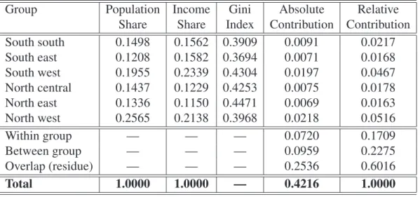
In table 2, we decompose the Gini index by the six Nigerian geopolitical zones. The contribution of the within group inequality to total poverty is less than that of the between group inequality11. The highest level of the overlap component
indi-cates also that the level of identification of groups, based on these six geopolitical zones, is low. One can recall here that the group identification by a given indica-tor, like the household income, is high when one can identify population groups only by using this indicator.
The decomposition of the FGT index by average per capita expenditures and inequality components across zones is presented in tables (3) and (4) for α = 0 and α = 1 respectively. The World Bank poverty line earlier mentioned is about twice the average per capita expenditures. This means that the contribution of the average standard of living is not nil. For the headcount index, inequality con-tributes positively to the total poverty if poverty line is lower than the average standard of living and contributes negatively if the poverty line exceeds this aver-age.
While the between group inequality contributes more to the total inequality measured by the Gini index, its contribution to total poverty is very low. This paradoxical result can be explained partially by the focus axiom that poverty in-dices obey. This means that poverty inin-dices are not sensitive to incomes that are higher than the poverty line. Indeed, when the within group inequality is removed and when the average income of each group is greater than the poverty line, the Gini index is not nil but the poverty index is equal to zero. With respect to the within group inequality components, one can remark that the northern zones con-tribute more than the southern zones.
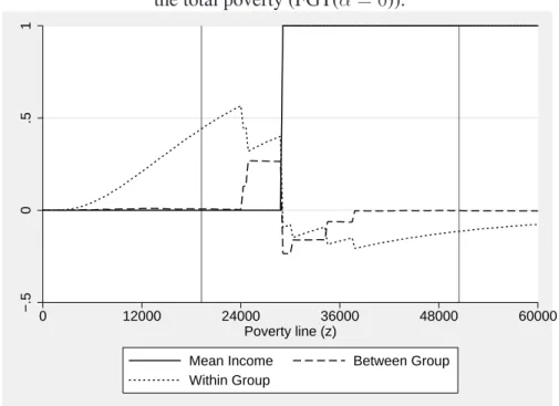
In figures 4 and 5, we display the magnitude of the contribution of each com-ponent according to the poverty line when the parameter α = 0 and α = 1. When the poverty line is below the average per capita expenditures, the contribution of this average is nil. For the headcount index, the contribution of inequality com-ponents is greater than zero when poverty line is below the average standard of living.
11The residue component is explained by the overlap group income. According to Araar (2006),
Nigeria presents an interesting case for the view of our development applica-tion. One can remark easily that the relative poverty line is very low (far from the World Bank poverty line). The policy implications of this would have far reach-ing effects. For instance, when the country is very poor and the poverty line is higher than the average standard of living, the explanatory power of inequality on poverty will be very low. In this case, the best policy option to fight poverty is to boost the economy by increasing per capita GDP. On the other hand, if the average standard of living is relatively higher than the poverty line, redistributive policies are appropriate for quick poverty alleviation.
To show how inequality of each income source contributes to the total poverty, we use the per capita income as the household standard of living. Since some households did not report their income sources, observations that contains miss-ing values were omitted and 17764 observations were used for this application. Inequalities of components Employment income and Non farm business income contribute more to total poverty than inequality in Agricultural income. Results of this decomposition can guide and inspire policy makers to formulate workable poverty reduction policies. For instance, a progressive income tax structure and introduction of subsidy program for some goods that are largely consumed by poor households will result in a sharp reduction of total poverty in Nigeria.
6 Conclusion
Explaining the persistence of poverty in developing countries continue to in-terest researchers and policy makers. Based on distributive analysis, two main factors can explain the level of poverty. The first is the average standard of living, which reflects the level of development of the country, while the second is the shape of the distribution of income. This paper is devoted to explore the link be-tween inequality and poverty. In this paper, some theoretical developments were provided to estimate the contribution of inequality components to total poverty. Inequality components can be the between and within group inequalities or in-equality in income sources. We have illustrated theoretical frameworks developed using the Nigerian Living Standard Survey for the year 2004. The main lesson drawn from these results is that redistributive policies cannot be the main tool to fight poverty when the country is very poor. Hence, the best option is to improve the general economic performance.
Figure 1: Density functions according to the Nigerian geopolitical zones Nigeria (2004) 0 .00001 .00002 .00003 .00004 .00005 f(y) 0 12000 24000 36000 48000 60000
Per capita expenditures
south south south east
south west north central
north east north west
Figure 2: FGT curves (α=0) according to the Nigerian geopolitical zones Nigeria (2004) 0 .2 .4 .6 .8 1 FGT(z, alpha = 0) 0 12000 24000 36000 48000 60000 Poverty line (z)
south south south east
south west north central
Figure 3: Lorenz curve, Gini index and poverty Nigeria (2004) 0 .2 .4 .6 .8 1 L(p) 0 .2 .4 .6 .8 1 Percentiles (p)
Inequality between groups Inequality within the poor group
Table 1: Decomposition of the FGT index according to the geopolitical zones. (α = 0; z = 19223 NG)
Group FGT Population Absolute Relative Index Share Contribution Contribution South south 0.4019 0.1498 0.0602 0.1343 South east 0.2435 0.1208 0.0294 0.0656 South west 0.3485 0.1955 0.0682 0.1520 North central 0.5211 0.1437 0.0749 0.1670 North east 0.5780 0.1336 0.0772 0.1721 North west 0.5401 0.2565 0.1386 0.3090 Total 0.4484 1.0000 0.4484 1.0000
Table 2: Decomposition of the Gini index according to the geopolitical zones. Group Population Income Gini Absolute Relative
Share Share Index Contribution Contribution South south 0.1498 0.1562 0.3909 0.0091 0.0217 South east 0.1208 0.1582 0.3694 0.0071 0.0168 South west 0.1955 0.2339 0.4304 0.0197 0.0467 North central 0.1437 0.1229 0.4253 0.0075 0.0178 North east 0.1336 0.1150 0.4471 0.0069 0.0163 North west 0.2565 0.2138 0.3968 0.0218 0.0516 Within group — — — 0.0720 0.1709 Between group — — — 0.0959 0.2275 Overlap (residue) — — — 0.2536 0.6016 Total 1.0000 1.0000 — 0.4216 1.0000
Figure 4: Contributions of the average expenditures and inequality components to the total poverty (FGT(α = 0)).
−.5 0 .5 1 0 12000 24000 36000 48000 60000 Poverty line (z)
Mean Income Between Group
Within Group
Figure 5: Contributions of the average expenditures and inequality components to the total poverty (FGT(α = 1)).
0 .1 .2 .3 .4 .5 0 12000 24000 36000 48000 60000 Poverty line (z)
Mean Income Between Group
T able 3: Decomposing the FGT inde x (α = 0) by av erage expenditures and inequality components P overty line = 2/ 3µ a P overty line = 1 $ U S b Components Absolute Relative Absolute Relative P opulation Contrib ution Contrib ution Contrib ution Contrib ution Shar e South south 0.0623 0.1390 -0.0183 -0.0206 0.1498 South east 0.0389 0.0868 -0.0185 -0.0210 0.1208 South west 0.0764 0.1704 -0.0282 -0.0318 0.1955 North central 0.0682 0.1521 -0.0150 -0.0169 0.1437 North east 0.0709 0.1582 -0.0092 -0.0104 0.1336 North west 0.1247 0.2780 -0.0249 -0.0281 0.2565 W ithin group (Sub-T ot.) 0.4414 0.9844 -0.1140 -0.1289 1.0000 Between group 0.0070 0.0156 -0.0012 -0.0013 — A verage income 0.0000 0.0000 1.0000 1.1302 — T otal 0.4484 1.0000 0.8848 1.0000 1.0000 a: Po verty line equals to tw o third of the av erage per capita expenditures (po verty line = 19223 NG). b: Po verty line equals to one US dollar . Exchange rate to US$1 (as of January ,2004) 138.21 (po verty line = 50446 NG).
T able 4: Decomposing the FGT inde x (α = 1) by av erage expenditures and inequality components P overty line = 2/ 3µ a P overty line = 1 $ U S b Components Absolute Relative Absolute Relative P opulation Contrib ution Contrib ution Contrib ution Contrib ution Shar e South south 0.0209 0.1238 0.0114 0.0222 0.1498 South east 0.0118 0.0698 0.0118 0.0230 0.1208 South west 0.0313 0.1851 0.0213 0.0414 0.1955 North central 0.0285 0.1690 0.0102 0.0199 0.1437 North east 0.0258 0.1529 0.0136 0.0265 0.1336 North west 0.0453 0.2684 0.0157 0.0306 0.2565 W ithin group (Sub-T ot.) 0.1636 0.9690 0.0841 0.1636 1.0000 Between group 0.0052 0.0310 0.0017 0.0033 — Mean income 0.0000 0.0000 0.4284 0.8331 — T otal 0.1689 1.0000 0.5142 1.0000 1.0000 a: Po verty line equals to tw o third of the av erage per capita expenditures (po verty line = 19223 NG). b: Po verty line equals to one US dollar . Exchange rate to US$1 (as of January ,2004) 138.21 (po verty line = 50446 NG).
T able 5: Decomposing the FGT inde x (α = 0) by av erage income and inequality components P overty line = 2/ 3 aver ag e income a P overty line = 1 $ U S b Components Absolute Relative Absolute Relative Income Concentr ation Contrib ution Contrib ution Contrib ution Contrib ution Shar e Inde x Emplo yment income 0.3517 0.5853 -0.0531 -0.0600 0.3530 0.7533 Agricultural income -0.0420 -0.0699 -0.0084 -0.0095 0.1999 0.3182 Fish processing income 0.0026 0.0044 -0.0020 -0.0023 0.0237 0.5262 Non farm business income 0.2834 0.4716 -0.0448 -0.0505 0.3441 0.6666 Remittances recei ved 0.0029 0.0047 -0.0015 -0.0017 0.0246 0.5622 All other income 0.0023 0.0038 -0.0046 -0.0052 0.0548 0.5727 Inequality component 0.6008 1.0000 -0.1145 -0.1292 A verage income component 0.0000 0.0000 1.0000 1.1292 T O T AL 0.6008 1.0000 0.8855 1.0000 1.0000 a: Po verty line equals to tw o third of the av erage income, (po verty line = 15610 NG). b: Po verty line equals to one US dollar . Exchange rate to US$1 (as of January ,2004) 138.21 (po verty line = 50446 NG).
Appendix A: The link between the headcount and the Gini Index
According to Runciman (1966), the magnitude of relative deprivation is the differ-ence between the desired situation and the actual situation of a person. We define the relative deprivation of household i compared to j as follows12:
δi,j = (yj − yi)+ =
½
yj − yi if yi < yj
0 otherwise. (A.1)
The expected deprivation of household i equals to:
¯ δi = N P j=1 (yj − yi)+ N (A.2)
The Gini coefficient can be written in the following form:
I = N X i=1 ¯ δi µyN = δ¯ µ (A.3)
For the inequality between the poor and the non poor groups, the expected depri-vation of the poor is:
¯
δp = (1 − H)(µnp− µp)
= µ − µp (A.4)
Thus, the between group Gini index equals to: ˜
I = 1
µH (µ − µp) (A.5)
This implies also:
H = µ ˜I µ 1 µ − µp ¶ (A.6)
Appendix B: The Shapley Value
Applied in several scientific domains, the Shapley approach can serve to per-form an exact decomposition of the distributive indices13. The Shapley value is a
solution concept often employed in the theory of cooperative games. Consider a set N of n players that must divide a given surplus among themselves. The play-ers may form coalitions (these are the subsets S of N) that appropriate themselves a part of the surplus and redistribute it between their members. The function v is assumed to determine the coalition force, i.e., which surplus will be divided without resorting to an agreement with the outsider players (the n − s − 1 players that are not members of the coalition S). The question to resolve is: How can the surplus be divided between the n players? According to the Shapley approach, introduced by Loyd. (1953), the value or the expected gain of player k, noted by
Ek, is shown by the following formula: Ek = X s⊂S s∈{0,n−1} s!(n − s − 1)! n! MV (S, k) (B.1) MV (S, k) = (v (S ∪ {k}) − v(S)) (B.2) The term MV (S, k) is the marginal value that the player k generates after his adhesion to the coalition S. What will then be the expected marginal contribution of player k, according to the different possible coalitions that can be formed and to which the player can adhere? First, the size of the coalition S is limited to:
s ∈ {0, 1, ...n − 1}. Suppose that the n players are randomly ordered and we note
the order by σ, such that:
σ = σ 1,σ2, · · · , σi−1 | {z } s , σi, σi+1, · · · , σn | {z } n−s−1 (B.3)
For each of the possible permutation of the n players, which equals n!, the number of times that the same first s players are located in the subset or coalition S is given by the number of possible permutations of the s players in coalition S (that is s!). For every permutation in the coalition S, one finds (n−s−1)! permutations for the players that complement the coalition S. The expected marginal value that player k generates after his adhesion to a coalition S is given by the Shapley
value. For every position of the factor k (predetermined cuts of the coalition S), there are several possibilities to form coalitions S from the n − 1 player (that is the n players without the player k). This number of possibilities is equal to the number of combinations, Cs
n−1.
How many marginal values would one have to compute to determine the ex-pected marginal contribution of a given factor or player k? Because the order of the players in the coalition S does not affect the contribution of the player k once he has adhered to the coalition, the number of calculations needed for the marginal values is: n−1P
s=0 Cs
n−1 = 2n−1. If we do not take into account this simplification, we
can write the extended formula of the Shapley Value as follows:
Ek = 1 n! n! X i=1 MV (σi, k) (B.4)
where for each order σ of the n! orders, the players k have only one position that determines the coalition to which he can adhere. The term MV (σi, k) equals
the marginal value of adding the player k to its coalition. The properties of the decomposition of this approach are:
• Symmetry, which ensures that the contribution of each factor is independent of its order of appearance on the list of the factors or the sequence.
References
ARAAR, A. (2006): “On the Decomposition of the Gini Coefficient: an Exact Approach, with an Illustration Using Cameroonian Data,” Tech. Rep. CIRPEE-WP:06-02.
DATT, G. AND M. RAVALLION (1992): “Growth and Redistribution
Com-ponents of Changes in Poverty Muasures: a Decomposition with Ap-plications to Brazil and India in the 1980’s,” Journal of Development
Economics, 38, 275–295.
DEININGER, K. AND L. SQUIRE (1998): “New Ways of Looking at Old
Issues: Inequality and Growth,” Journal of Development Economics, 38, 259–87.
FELDSTEIN, M. (1998): “Income Inequality and Poverty,” Tech. Rep. WP-6770, NBER, Cambridge.
FIELDS, G. S. (1989): “Changes in Poverty and Inequality in Developing Countries,” World Bank Res Obs, 4, 167–185.
HEY, J. D. ANDP. J. LAMBERT(1980): “Relative Deprivation and the Gini Coefficient: Comment,” Quarterly Journal of Economics, 95, 567–573.
KAKWANI, N. (1997): “On measuring Growth and Inequality Components
of Changes in Poverty with Application to Thailand,” Discussion paper 97/16, The University of New South Wales.
KAKWANI, N., S. KHANDKER, AND H. SON (2003): “Poverty
Equiva-lent Growth Rate: With Applications to Korea and Thailand,” Tech. rep., Economic Commission for Africa.
KUZNETS, S. (1956): “Economic Growth and Income Inequality,”
Ameri-can Economic Review, 45, 1–28.
LAMBER, P. J. AND J. R. ARONSON (1993): “Inequality Decomposition
Analysis and the Gini Coefficient Revisited,” Economic Journal, 103, 1221–1227.
LOYD., S. (1953): A Value for n-Person Games, in Contributions to the
The-ory of Games II (Annals of Mathematics Studies), Princeton University
Press.
RAVALLION, M.AND S. CHEN (1997): “What Can New Survey Data Tell
Us about Recent Changes in Distribution and Poverty?” World Bank
——— (2003): “Measuring Pro-poor Growth,” Economics Letters, 78, 93– 99.
RAVALLION, M.ANDG. DATT(2002): “Why Has Economic Growth Been
More Pro-poor in Some States of India Than Others?” Journal of
Devel-opment Economics, 68, 381–400.
RUNCIMAN, W. G. (1966): Relative Deprivation and Social Justice: A
Study of Attitudes to Social Inequality in Twentieth-Century England,
Berkeley and Los Angeles: University of California Press.
SHORROCKS, A. (1999): “Decomposition procedures for distributional
analysis: A unified framework based on the Shapley value,” Tech. rep., University of Essex.
SON, H. (2004): “A note on pro-poor growth,” Economics Letters, 82, 307– 314.
YITZHAKI, S. (1979): “Relative Deprivation and the Gini Coefficient,”