Uncertainty in East Antarctic firn thickness constrained using a model ensemble
approach
V. Verjans1, A. A. Leeson1, M. McMillan1, C. M. Stevens2,3,4, J. M. van Wessem5, W. J. van
de Berg5, M. R. van den Broeke5, C. Kittel6, C. Amory6,7, X. Fettweis6, N. Hansen8,9, F.
Boberg8 and R. Mottram8
1Lancaster Environment Centre, Lancaster University, Lancaster, LA1 4YQ, UK. 2Department of Earth and Space Sciences, University of Washington, Seattle, WA, USA 3Earth System Science Interdisciplinary Center, University of Maryland, College Park, MD,
USA
4Department NASA Goddard Space Flight Center, Greenbelt, MD, USA
5Institute for Marine and Atmospheric research Utrecht, Utrecht University, Utrecht, the
Netherlands
6Laboratory of Climatology, Department of Geography, SPHERES research unit, University of
Liège, Liège, Belgium
7Univ. Grenoble Alpes, CNRS, Institut des Géosciences de l'Environnement, Grenoble, France 8Danish Meteorological Institute, Lyngbyvej 100, Copenhagen, 2100, Denmark
9DTU Space, Department of Geodynamics, Technical University of Denmark, Kongens Lyngby,
Denmark
Corresponding author: Vincent Verjans ([email protected])
Key Points:
• By developing an ensemble of 54 model scenarios, we constrain firn thickness change uncertainty in East Antarctica over 1992-2017.
• In 9 of 16 basins, modelled firn thickness and altimetry trends agree; elsewhere uncertainty is underestimated or ice flow imbalance exists.
• Model uncertainty reaches 1 cm yr-1 with snowfall, firn compaction and snow density
having spatially variable contributions to uncertainty.
Accepted
Accepted
Article
Abstract
Mass balance assessments of the East Antarctic ice sheet (EAIS) are highly sensitive to changes in firn thickness, causing substantial disagreement in estimates of its contribution to sea-level. To better constrain the uncertainty in recent firn thickness changes, we develop an ensemble of 54 model scenarios of firn evolution between 1992-2017. Using statistical emulation of firn-densification models, we quantify the impact of firn compaction formulation, differing climatic forcing, and surface snow density on firn thickness evolution. At basin scales, the ensemble uncertainty in firn thickness change ranges between 0.2–1.0 cm yr-1 (15–300% relative
uncertainty), with the choice of climate forcing having the largest influence on the spread. Our results show the regions of the ice sheet where unexplained discrepancies exist between observed elevation changes and an extensive set of modelled firn thickness changes estimates, marking an important step towards more accurately constraining ice sheet mass balance.
Plain Language Summary
Firn is the transition stage between snow and ice. The total thickness of the firn layer varies in time and space. In East Antarctica, uncertainty about this variability has a large impact on satellite-based estimates of ice sheet mass change. We combine statistical surrogates of firn-densification models with different climate models over the entire East Antarctic ice sheet. Our ensemble of model combinations demonstrates that firn thickness estimates are poorly
constrained. Accounting for their respective uncertainties, modelled firn thickness change and satellite measurements of elevation change are consistent over most of East Antarctica. However, we identify several areas of mismatch between model estimates and elevation change
observations, which likely indicates that further improvements are required either in models or in measurement techniques. Alternatively, these disagreements can hint at possible imbalances in the flow of ice, below the firn layer. We quantify how much different sources of uncertainty contribute to the total uncertainty in modelled firn thickness change. The amount of snowfall estimated by climate models mostly dominates the uncertainty, but modelled firn compaction rates and uncertainty in surface snow density also have major contributions in certain areas.
1 Introduction
The Antarctic ice sheet (AIS) is the largest ice body on Earth, holding a total potential contribution to sea-level rise of ~57.2 m (Rignot et al., 2019). The AIS is divided into three entities: the Antarctic Peninsula (AP) and the West and East Antarctic ice sheets (WAIS and EAIS, respectively). The EAIS has shown less dynamic instabilities than the WAIS and AP over the past four decades, but it holds ~90% of the total AIS ice mass and is the area with highest uncertainty concerning recent mass trends (Shepherd et al., 2018; Rignot et al., 2019). A layer of firn, the intermediary stage between snow and ice, covers ~99% of the AIS (Winther et al., 2001). The firn layer thickness, defined here as the depth from the surface until the firn-ice transition, varies from 0 to more than 100 m (van den Broeke, 2008). Firn thickness also fluctuates in time due to changes in firn compaction rates and climatic conditions, primarily net snow accumulation. These fluctuations affect ice sheet mass balance assessments derived from satellite-based altimetry. Measured surface elevation changes are converted into mass changes, but the conversion requires precise knowledge of variability in firn thickness and mass.
Accepted
Article
Atmospheric reanalysis products, Regional Climate Models (RCMs) and Firn Densification Models (FDMs) are therefore used to simulate changes of firn properties and, ultimately, to evaluate ice sheet mass changes with precision (Li and Zwally, 2011; Kuipers Munneke et al., 2015; McMillan et al., 2016; Shepherd et al., 2019; Smith et al., 2020).
By simulating mass fluxes (snowfall, sublimation, melt), RCMs estimate the surface mass balance (SMB) of ice sheets, which partly determines the evolution of the firn layer. These fluxes and modelled surface temperatures also serve as input forcing for FDMs that explicitly simulate firn compaction rates. Such coupling is required to reproduce seasonal and multi-annual fluctuations in compaction rates (Arthern et al., 2010). Uncertainty in SMB estimates across Antarctica are typically assessed by comparing outputs from different RCMs. While SMB is key to firn thickness evolution because it determines the amount of snow removed and added at the surface, it does not capture the effects of fluctuating firn compaction that must be estimated with FDMs. Differences between FDMs can lead to substantial spread in modelled firn thickness and air content (Lundin et al., 2017), especially if scaled up to ice sheet extent.
Compared to the AP and the WAIS, observed elevation changes across the EAIS over the past 25 years have been generally smaller, and largely driven by snowfall and compaction variability (Davis et al., 2005; Shepherd et al., 2018; Shepherd et al., 2019). Altimetry-derived mass balance assessments of the EAIS are very sensitive to estimates of firn thickness fluctuations because these are of the same order of magnitude as measured elevation changes. This sensitivity
complicates the interpretation of altimetry measurements in this area, and it is unclear whether to attribute elevation changes to ice dynamical imbalance or firn thickness change (Zwally et al., 2015; Scambos and Shuman, 2016; Shepherd et al., 2018). These conflicting assessments
motivate precise uncertainty analyses of coupled RCM-FDM systems over the EAIS. Previously, such analyses have been computationally limited; running multiple FDMs for many years at the spatial resolution of RCM grids over the EAIS requires many thousands of simulations. The extent to which estimates of firn thickness change vary by combining different FDMs with different RCMs remains an open question.
To overcome computational limitations and thus improve evaluation of uncertainty in the evolution of firn thickness, we build statistical emulators of nine FDMs. An emulator is a fast and statistically-driven approximation of a more complex physical model (Sacks et al., 1989; O'Hagan 2006). By combining the FDM emulators with climatic output from three state-of-the-art polar RCMs, we develop an ensemble of 54 scenarios of EAIS firn thickness change. We exploit these scenarios to constrain uncertainty analyses of firn thickness fluctuations on the EAIS and to quantify the contributions of various sources of uncertainty to the spread of modelled results.
Accepted
Article
2 Methods
2.1 Ensemble configuration
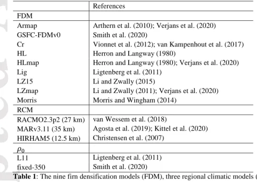
To generate our ensemble, we first calibrate each of the nine FDM emulators to its corresponding FDM (Table 1) in a representative range of EAIS climate conditions, and then we use it to
emulate compaction rates across the entire EAIS. Changes in SMB as well as climatic forcing for the emulators are computed from three RCMs: RACMO2, MAR and HIRHAM (Table1). Our modelled scenarios of firn thickness change span the 1992-2017 period. This period is chosen to match the long-term altimetry record of Shepherd et al. (2019), hence facilitating
intercomparison of observed elevation changes and modelled firn thickness change experiments of this study. We limit our analysis to the EAIS because surface melt there is minor compared to the AP and WAIS, and FDM fidelity remains questionable for simulating wet firn compaction, water percolation and refreezing (Steger et al., 2017; Verjans et al., 2019; Vandecrux et al., 2020).
References FDM
Armap Arthern et al. (2010); Verjans et al. (2020)
GSFC-FDMv0 Smith et al. (2020)
Cr Vionnet et al. (2012); van Kampenhout et al. (2017)
HL Herron and Langway (1980)
HLmap Herron and Langway (1980); Verjans et al. (2020)
Lig Ligtenberg et al. (2011)
LZ15 Li and Zwally (2015)
LZmap Li and Zwally (2011); Verjans et al. (2020)
Morris Morris and Wingham (2014)
RCM
RACMO2.3p2 (27 km) van Wessem et al. (2018)
MARv3.11 (35 km) Agosta et al. (2019); Kittel et al. (2020)
HIRHAM5 (12.5 km) Christensen et al. (2007)
L11 Ligtenberg et al. (2011)
fixed-350 Smith et al. (2020)
Table 1: The nine firn densification models (FDM), three regional climatic models (RCM) and two surface density
parameterisations ( ) used in this study. The horizontal resolutions of the RCM grids are given in brackets. All
RCMs were forced by the ERA-Interim reanalysis at their boundaries (Dee et al., 2011). See Supplementary Information for details on the FDMs.
2.2 Firn thickness change calculations
Observed ice sheet elevation changes, once corrected for glacial isostatic adjustment, are composed of two different signals: one related to ice dynamical imbalance and one to firn
thickness change. In this study, we focus on the latter. The change in firn thickness at time step ,
ℎ ( ), is given by:
Accepted
Article
with all components expressed in metres and considered positive, and set to a daily time step in this study. The subscript refers to surface firn removal by melting and refers to net snow accumulation. Both ℎ and ℎ depend on the RCM-computed mass fluxes and on the value assumed for surface snow density, but they are independent of FDM calculations. The
component ℎ is the emulated firn compaction term (Section 2.3). The last component, ℎ , quantifies changes in the flux through the lower boundary of the firn column and thus captures changes in the rate of conversion from firn to ice. Changes in ℎ act on much longer
timescales than the other components (Zwally and Li, 2002; Kuipers Munneke et al., 2015). As such, ℎ can be set constant and equal to the average rate of conversion from firn to ice over a reference period (we use 1979-2009, following Ligtenberg et al., 2011), ℎ . By assuming firn thickness in steady state, thus without trend, over the reference period, ℎ balances the reference period averages of the other components:
ℎ = ℎ − ℎ − ℎ (2)
Substituting ℎ for ℎ in Eq. (1) yields Eq. (3). This is equivalent to calculating firn thickness change by computing anomalies in each of the , and components with respect to their average value in the reference period (Li and Zwally, 2015).
ℎ ( ) = ℎ ( ) − ℎ ( ) − ℎ ( ) − ℎ (3)
In this study, we are interested in the cumulative 1992-2017 firn thickness changes. We thus integrate Eq. (3) over this time period to compute a total firn thickness change ℎ .
2.3 Emulation of firn compaction
The nine FDM emulators are first calibrated at 50 sites on the EAIS and over the entire time span (1979-2017) covered by the output of RCMs (Supplementary Information for details). The goal of the emulation is to capture both long- and short-term sensitivity of ℎ to climatic forcing. The long-term (1979-2017) mean and trend in ℎ are estimated by linear regressions on the long-term means and trends of temperature, accumulation and melt. These linear regressions are specific to each FDM and show good performance in capturing the FDM-computed means and trends at the calibration sites (R2>0.99 and R2>0.97 respectively). Gaussian Process regression
complements the linear regression by capturing short-term fluctuations from the long-term trends as a function of detrended values of temperature and accumulation. We evaluate the emulation capabilities in a leave-one-out cross-validation framework; the nine FDM emulators reproduce the FDM output well, both for the total 1979-2017 ℎ (R2>0.99, RMSE=0.49 m, corresponding
to 3.5% of the mean total ℎ ) and for daily values (R2>0.99, RMSE=0.15×10⁻³ m)
(Supplementary Information for details).
2.4 Uncertainty contributions
In order to evaluate uncertainty on the time series of cumulative ℎ ( ) and on ℎ , we construct a model ensemble; the spread arising from a large number of simulations provides an estimate of uncertainty (e.g. Déqué et al, 2007). Our ensemble includes all combinations of the nine FDM emulators and the three RCMs (Table 1). Furthermore, surface snow density, ,
Accepted
Article
contributes to uncertainty in all components of ℎ (e.g. Ligtenberg et al., 2011; Agosta et al., 2019). As such, we use two different possibilities for the value of : the climate-dependent parameterisation of Ligtenberg et al. (2011) and the approach of Smith et al. (2020), which takes a constant value of 350 kg m-3 (B. Medley, personal communication, 2020) (Table 1). The
different combinations of RCM, FDM and provide 54 different firn thickness change scenarios across the EAIS. We refer to the spread in the model ensemble results as the total ensemble uncertainty to distinguish it from the true uncertainty, which may not be captured by the ensemble. We then use the analysis of variance (ANOVA) theory to partition the total ensemble uncertainty among the three factors RCM, FDM and (von Storch and Zwiers, 1999; Déqué et al., 2007; Yip et al., 2011). This approach allows us to decompose the variance in model results into the contribution of each factor and of each interaction between these factors (Eq. (4)).
= + + + + + + (4)
where is the variance in the ensemble results (m2) and the terms are the contributions from
each factor and interaction between factors to . Interaction effects stem from a non-linear behaviour of the three uncertainty sources. Contributions are calculated by computing the sum of squares associated with each term.
! " # " $ =&%'∑ ()..− )…) &' ,%
- =&'% &/∑ ∑ 0)&,%' -,%&/ -.− ) ..− ).-.+ )…1
- 2 =&' &%/ &3∑ ∑&,%' -,%&/ ∑&2,%3 0)-2− )-.− ).2− ).-2+ )..+ ).-.+ )..2− )…1
(5)
where 4 denotes the number of possible levels for a factor (3 for RCMs, 9 for FDMs, 2 for ),
) denotes the value of the variable of interest ( ℎ ) and a dot represents the arithmetic mean
with respect to the index it is substituted for. Because the sums of squares in Eq. (5) are averaged departures from a mean, these terms are biased estimates of the variance (Déqué et al., 2007). An unbiased estimate should be divided by 4 − 1, but dividing by 4 results in terms fulfilling Eq. (4). As such, any ratio / is only interpreted as a percentage of contribution to the total ensemble uncertainty. We group together all terms capturing an interaction effect to quantify the non-linear behaviour of the model experiments with respect to the three factors ( 7 ).
Accepted
Article
3 Results
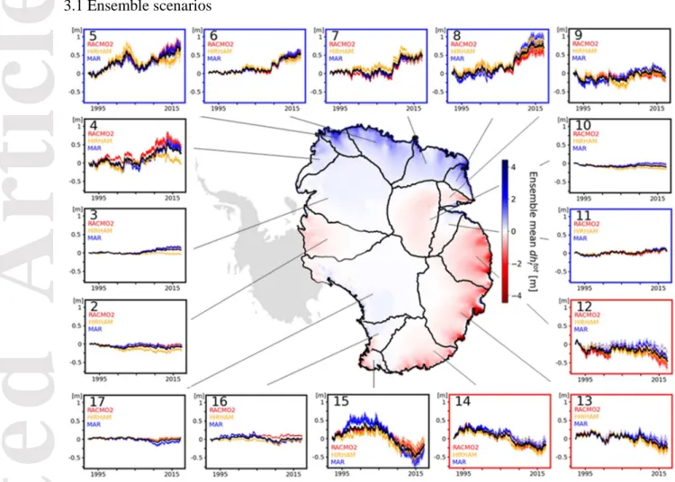
3.1 Ensemble scenarios
Figure 1: Ensemble mean 1992-2017 firn thickness change ( ℎ ) in each EAIS basin. Simulation results are
interpolated by nearest-neighbour to a common 12.5 km grid. The map uses a 3×3 median filter. Each inset shows the basin-averaged modelled time series of all the 54 model scenarios. Red, yellow and blue curves represent scenarios forced with RACMO2, HIRHAM and MAR respectively. Each curve represents a particular
combination. The thick black curve represents the ensemble mean. Basin numbers are displayed within the insets.
Frame colours show whether ℎ is significantly positive (blue), negative (red) or not significantly different from
zero (black) (at ±2 ). Basin limits follow Zwally et al. (2015).
The model ensemble shows a stable firn thickness over 1992-2017 for most of the EAIS, but strong regional changes are evident in several of the 16 basins (Figure 1). The large interior basins (2, 3, 10, 17) show no significant thickness change; the 9: uncertainty ranges of the ensemble results encompass zero. In contrast, the ensemble shows a significant and pronounced (>0.49 m) firn thickening in Dronning Maud Land (basins 5-8), driven by high snowfall rates since 2009 (Boening et al., 2012; Medley et al., 2018). Conversely, decreases in snowfall rates cause firn thinning (>0.25 m) in the areas of Shackleton ice shelf and Totten glacier (basins 12-13), which coincide with localised zones of high ice flow velocities (Rignot et al., 2019). Low accumulation since 2005 also induced thinning in Victoria Land (basin 14) (Velicogna et al., 2014). In such cases of accumulation anomalies, the firn compaction signal must be accounted
Accepted
Article
for as it partially mitigates the overall change in firn thickness; increased accumulation provides more pore space and thus higher compaction rates, while decreased accumulation has the opposite effect. In other basins, the ensemble suggests thickening (e.g. basins 3-4) or thinning (e.g. basins 9 and 15) but high variability among model scenarios precludes any firm conclusion.
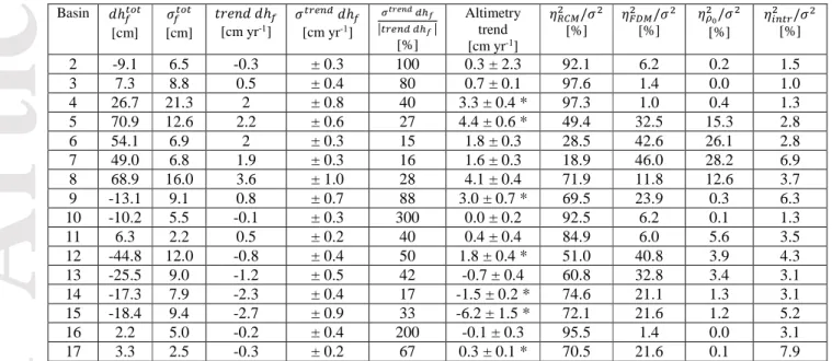
Basin ℎ [cm] [cm] ;<= ℎ [cm yr-1] 7> ℎ [cm yr-1] ?@ABCD >EF G 7> >EF G [%] Altimetry trend [cm yr-1] / [%] / [%] / [%] 7 / [%] 2 -9.1 6.5 -0.3 ± 0.3 100 0.3 ± 2.3 92.1 6.2 0.2 1.5 3 7.3 8.8 0.5 ± 0.4 80 0.7 ± 0.1 97.6 1.4 0.0 1.0 4 26.7 21.3 2 ± 0.8 40 3.3 ± 0.4 * 97.3 1.0 0.4 1.3 5 70.9 12.6 2.2 ± 0.6 27 4.4 ± 0.6 * 49.4 32.5 15.3 2.8 6 54.1 6.9 2 ± 0.3 15 1.8 ± 0.3 28.5 42.6 26.1 2.8 7 49.0 6.8 1.9 ± 0.3 16 1.6 ± 0.3 18.9 46.0 28.2 6.9 8 68.9 16.0 3.6 ± 1.0 28 4.1 ± 0.4 71.9 11.8 12.6 3.7 9 -13.1 9.1 0.8 ± 0.7 88 3.0 ± 0.7 * 69.5 23.9 0.3 6.3 10 -10.2 5.5 -0.1 ± 0.3 300 0.0 ± 0.2 92.5 6.2 0.1 1.3 11 6.3 2.2 0.5 ± 0.2 40 0.4 ± 0.4 84.9 6.0 5.6 3.5 12 -44.8 12.0 -0.8 ± 0.4 50 1.8 ± 0.4 * 51.0 40.8 3.9 4.3 13 -25.5 9.0 -1.2 ± 0.5 42 -0.7 ± 0.4 60.8 32.8 3.4 3.1 14 -17.3 7.9 -2.3 ± 0.4 17 -1.5 ± 0.2 * 74.6 21.1 1.3 3.1 15 -18.4 9.4 -2.7 ± 0.9 33 -6.2 ± 1.5 * 72.1 21.6 1.2 5.2 16 2.2 5.0 -0.2 ± 0.4 200 -0.1 ± 0.3 95.5 1.4 0.0 3.1 17 3.3 2.5 -0.3 ± 0.2 67 0.3 ± 0.1 * 70.5 21.6 0.1 7.9
Table 2: For each EAIS basin, ensemble mean ( ℎ ) and standard deviation ( ) of firn thickness change. Mean (;<= ℎ ) and standard deviation ( 7> ℎ) of the linear trends fitted to the ensemble scenarios, and their ratio (G?@ABCD7> >E >EF
F G). Altimetry trends are from Shepherd et al. (2019). Superscript * denotes non-overlapping uncertainty
ranges from altimetry and from the model ensemble. / ratios show contributions of the sources of uncertainty
to the ensemble spread.
Model uncertainties in basin-averaged rates of firn thickness change range between 0.2–1.0 cm yr-1, translating into relative uncertainties between 15–300% (Table 2). Despite low absolute
uncertainties, the interior basins (2, 3, 10, 16, 17) show the largest relative values because their trends in ℎ are close to zero (<0.4 cm yr-1). Basins with trends exceeding 1 cm yr-1 have lower
relative uncertainties. Yet, some of these still exhibit relative uncertainties higher than 25% (4, 5, 8, 13, 15). The relative importance of the RCM, FDM and factors on the model spread varies between basins. An area-weighted averaging demonstrates the general predominance of the RCM factor (72%) followed by the FDM (20%), (4%) and interaction (4%) factors. The high influence of RCM choice is mostly due to the large and direct impact of SMB on firn thickness. In addition, there is an indirect impact of RCM output as forcing for FDMs and for the climate-dependent L11 parameterisation of .
Cold basins with low snowfall rates (e.g. 2-3, 10-11) are characterised by particularly high contributions of (>90% of ). In such dry conditions, small discrepancies between RCM-modelled snowfall anomalies translate into large relative differences in firn thickness change. FDM contribution to the total ensemble uncertainty increases in basins with higher temperature and accumulation (e.g. 5-7, 12-13), with explaining approximately 30 to 45% of the spread. These climatic settings drastically increase both the sensitivity of FDMs to temperature
Accepted
Article
fluctuations and the absolute compaction rates. Consequently, small relative differences in compaction rates between the FDMs result in large absolute differences in firn thickness change. Moreover, high total snowfall amounts mitigate the impact of small differences between RCM estimates of accumulation, thus reducing . Another aspect that favours high / values is spatial variability of climatic conditions within basins; within basins spanning many climatic zones, there is more likely to be a region in which the FDMs disagree on compaction rates. Contribution of is highest in basins with large and positive snowfall anomalies (basins 5-8). In such basins, it accounts for up to 28% of the model spread because the thickening caused by the anomaly is sensitive to the snow density parameterisation. Basins 16 and 17 illustrate the role of interaction effects. In these basins, MAR simulates substantially higher temperatures and accumulation rates, causing larger disagreements between FDMs forced by MAR than between FDMs forced by RACMO2 or HIRHAM. This nonconstancy of variance across FDMs for different RCMs leads to a significant interaction term 7 . Because interaction effects account for a non-negligible part of the model spread in all basins (1 to 8% of ), our results
demonstrate the importance of combining RCMs, FDMs and within different model experiments to assess firn thickness change uncertainty.
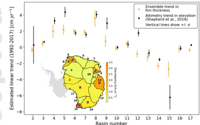
3.2 Comparison with altimetry
Figure 2: Comparison of 1992-2017 altimetry-based elevation trends and firn thickness trends of the ensemble, with
their respective 1 uncertainty ranges. Map shows the absolute ensemble-altimetry differences, crosses highlight basins with non-overlapping uncertainty ranges.
We compare our estimates of basin-wide trends in firn thickness with elevation trends reported by Shepherd et al. (2019) (Table 2, Figure 2). Firn thickness change is only a single component
Accepted
Article
of the ice sheet elevation change signal, which also captures ice dynamical imbalance. Thus, accurate estimations of firn thickness change can be compared to measured elevation changes to identify areas of dynamical imbalance (Li and Zwally, 2011; Kuipers Munneke et al., 2015; Hawley et al., 2020). For 9 of the 16 basins, the model ensemble uncertainty ranges and the altimetry uncertainty ranges overlap. In these cases, our results provide no evidence to support the existence of net ice flow imbalance. However, basin-wide averaging may conceal localised dynamic changes. On Totten glacier (within basin 13) for example, ice dynamical imbalance close to the grounding line makes a substantial contribution to recent mass loss and thus to local elevation decrease (Li et al., 2016). On the other hand, the uncertainty ranges do not overlap for several basins, highlighting the need to better understand the source of the discrepancies in these regions. In such cases, three possibilities, or combinations thereof, should be considered: (1) the model ensemble may fail to represent the true firn thickness change over the 1992-2017 period, (2) the 1: uncertainty range associated with the altimetry measurements may not adequately capture the true signal or (3) a component of the elevation changes may be related to ice dynamical imbalance.
At this stage, identifying the exact cause of the discrepancy remains speculative. The long response time of ice flow makes any dynamical imbalance challenging to evaluate because long-term trends may still outweigh recent changes (Zwally et al., 2015). Moreover, disagreements persist between simulated SMB and field observations in certain regions (Wang et al., 2016), which can lead to substantial differences in mass balance partitioning (Martin-Español et al., 2017; Mohajerani et al., 2019). Similarly, different sources of altimetry data, inter-satellite bias correction, and other processing steps induce uncertainty in altimetry signals (Shepherd et al., 2019). We use several basins where ensemble- and altimetry-based trends disagree to illustrate these factors. In basins 4 and 5, Medley et al. (2018) demonstrated that global climate models underestimate recent increases in snowfall. A similar underestimation from the RCMs used here would explain the lower ensemble trend compared to the observed elevation trend. In basin 12, significant changes in ice discharge may hint at a dynamic imbalance causing the disagreement (Rignot et al., 2019). However, this area also shows major discrepancies in SMB anomalies from different model estimates (Wang et al., 2016) and from probabilistic inversion techniques
(Martin-Español et al., 2017), suggesting that modelling SMB in this region is challenging. Basin 15 is characterised by sparse satellite sampling but also shows a large spread in our model ensemble and is thus poorly constrained. The relatively high model- and altimetry-uncertainties may both be related to the complex topography of this basin. Finally, a robust evaluation of FDM-reliability in all possible EAIS areas and climatic conditions does not exist and models may fail to predict true compaction rates. The objective of comparing ensemble firn thickness trends and altimetry trends is not to draw hasty conclusions about dynamical imbalance, but rather to highlight areas which deserve greater attention because recent measurements and current state-of-the-art model scenarios do not match.
In critically evaluating our work, it is important to highlight sources of uncertainty that are not accounted for in the ensemble. We use three RCMs forced by ERA-Interim at their boundaries. Different atmospheric reanalyses could, in theory, be used to force the RCMs or could be directly taken over the EAIS domain itself. Both the L11 and fixed-350 parameterisations of HI assume a time-invariant surface density because possible seasonal and interannual variabilities are unknown. The ensemble is limited by the deterministic RCM, FDM and HI combinations considered here. In the future, the work could be extended to consider stochastic perturbations
Accepted
Article
and parametric uncertainties in climate input, FDMs and HI, thereby providing a larger range of results. In principle, the process of emulation might lead to localised discrepancies between the emulator and a corresponding FDM, although evaluation (Supplementary Information) shows that this is unlikely when averaged over large spatial areas, as is done here. One critical
assumption is the reference climatic period of 1979-2009. Different ice core analyses and model-based studies disagree on the existence of a trend in Antarctic SMB over the last decades and centuries, but several agree on existing regional trends (Monaghan et al., 2006; Frezzotti et al., 2013; Previdi and Polvani, 2016; Medley and Thomas, 2019). The year 1979 coincides with the start of satellite data assimilation into atmospheric products, and thus with the earliest RCM output, motivating this choice of reference period for practical reasons (e.g. Ligtenberg et al., 2011; Rignot et al., 2019). However, we cannot discount that substantially lower/higher past accumulation rates would result in under/over-estimating recent firn thickness change, thus providing a possible cause of disagreement with elevation change measurements. Nevertheless, because all model scenarios use the same reference period, it has a minor impact on both the total ensemble uncertainty and the uncertainty partitioning; using another reference period could shift the estimates of each scenario but would affect differences between the estimates only
marginally.
4 Conclusions
Our model ensemble experiment provides a range of modelled scenarios of 1992-2017 firn thickness change on the EAIS that encompass current state-of-the-art modelling capabilities. Using statistical emulation of firn model output, we compute a total of 54 scenarios to assess variability associated with different RCMs, FDMs and surface snow density parameterisations. The ensemble agrees that firn thickness changes in the interior are minor, but there are
pronounced thickening and thinning patterns in coastal areas. At basin-level, the uncertainty on the model estimates ranges between 0.2–1.0 cm yr-1 and is generally dominated by differences
between RCMs due to the strong and direct effect of SMB on firn thickness. However, in basins with high snowfall and with large spatial variability of climatic conditions, FDM-related
variability increases up to 46% of the total ensemble uncertainty. The surface snow density factor has a large impact on uncertainty in basins with recent increases in snowfall rates, reaching a maximum contribution of 28%. Finally, non-linear interactions between the three sources of uncertainty are substantial across the EAIS. Our results demonstrate that refining SMB estimates in RCMs is the priority for constraining future assessments of firn thickness change. However, as snowfall and temperatures are expected to increase in Antarctica (Ligtenberg et al., 2013; Lenaerts et al., 2019), FDMs and snow density will increasingly contribute to model uncertainty and should not be neglected. By comparing the ensemble scenarios with satellite measurements of elevation changes over the same 1992-2017 period, we find that these estimates are consistent over a majority of basins. Nonetheless, we identify several basins where model estimates do not match altimetry measurements. While ice
dynamical imbalance could be the source of the discrepancies in these regions, so too could be inadequacies in the respective uncertainty characterisations. As such, our analysis serves to
Accepted
Article
highlight specific areas where further focus on potential sources of errors in model and altimetry results is needed in order to better constrain mass balance assessments in East Antarctica. Acknowledgments
We thank Andrew Shepherd for constructive discussions about our results. AL acknowledges support from EPSRC, A Data Science for the Natural Environment (EP/R01860X/1). MM was supported by the UK Natural Environment Research Council Centre for Polar Observation and Modelling (grant number cpom300001). MvdB acknowledges support from the Netherlands Earth System Science Centre (NESSC). We thank editor Mathieu Morlighem, reviewer Eric Keenan and one anonymous reviewer for providing insightful comments and for their handling of the review process.
All the modelled annually-averaged firn thickness change time series of this study are available at: https://doi.org/10.5281/zenodo.4515142. All the altimetry data shown in Table 2 and Figure 2 are from Table 1 in Shepherd et al. (2019).
References
Agosta, C., Amory, C., Kittel, C., Orsi, A., Favier, V., Gallée, H., et al. (2019). Estimation of the Antarctic Surface Mass Balance Using the Regional Climate Model MAR (1979–2015) and Identification of Dominant Processes. The Cryosphere, 13(1), 281–296. https://doi.org/ 10.5194/tc-13-281-2019
Arthern, R. J., Vaughan, D. G., Rankin, A. M., Mulvaney, R., & Thomas, E. R. (2010). In situ measurements of Antarctic snow compaction compared with predictions of models. Journal of Geophysical Research, 115, F03011. https://doi.org/10.1029/2009JF001306
Boening, C., Lebsock, M., Landerer, F., & Stephens, G. (2012). Snowfall‐driven mass change on the East
Antarctic ice sheet. Geophysical Research Letters, 39, L21501. https://doi.org/10.1029/2012GL053316 Christensen, O. B., Drews, M., Christensen, J. H., Dethloff, K., Ketelsen, K., Hebestadt, I., & Rinke, A. (2006). The
HIRHAM regional climate model, version 5 (Technical Report No. 06 17). Danish Meteorological ‐
Institute, Copenhagen, Denmark
Davis, C. H., Li, Y., McConnell, J. R., Frey, M. M., & Hanna, E. (2005). Snowfall-driven growth in East Antarctic
Ice Sheet mitigates recent sea-level rise. Science, 308, 1898–1901. doi:10.1126/science.1110662
Dee, D. P., Uppala, S. M., Simmons, A. J., Berrisford, P., Poli, P., Kobayashi, S., et al. (2011). The ERA Interim ‐
reanalysis: Configuration and performance of the data assimilation system. Quarterly Journal of the Royal
Meteorological Society, 137(656), 553–597. https://doi.org/ 10.1002/qj.828
Déqué, M., Rowell, D. P., Lüthi, D., Giorgi, F., Christensen, J. H., Rockel, B., et al. (2007). An intercomparison of regional climate simulations for Europe: Assessing uncertainties in model projections. Climatic Change,
81(S1), 53–70. https://doi.org/10.1007/s10584 006 9228 x‐ ‐ ‐
Frezzotti, M., Scarchilli, C., Becagli, S., Proposito, M., & Urbini, S. (2013). A synthesis of the Antarctic surface mass balance during the last 800 yr. The Cryosphere, 7(1), 303–319. https://doi.org/10.5194/tc-7-303-2013 Hawley, R. L., Neumann T. A., Stevens, C. M., Brunt. K. M., & Sutterley T. C. (2020). Greenland Ice Sheet
Elevation Change: Direct Observation of Process and Attribution at Summit. Geophysical Research
Letters. https://doi.org/10.1029/2020GL088864
Herron, M. M., & Langway, C. C. (1980). Firn densification: An empirical model. Journal of Glaciology, 25(93), 373–385. https://doi.org/ 10.3189/S0022143000015239
Kittel, C., Amory, C., Agosta, C., Jourdain, N. C., Hofer, S., Delhasse, A., et al. (2020). Diverging future surface mass balance between the Antarctic ice shelves and grounded ice sheet, The Cryosphere Discussion, https://doi.org/10.5194/tc-2020-291
Kuipers Munneke, P., Ligtenberg, S. R. M., Noël, B. P. Y., Howat, I. M., Box, J. E., Mosley Thompson, E., ‐ et al.
Accepted
Article
2014. The Cryosphere, 9(6), 2009–2025. https://doi.org/ 10.5194/tc 9 2009 2015
Lenaerts, J. T. M., Medley, B., van den Broecke, M. R., & Wouters, B. (2019). Observing and modeling ice sheet surface mass balance. Reviews in Geophysics, 57, 376–420. https://doi.org/10.1029/2018RG000622 Li, J., & Zwally, H. J. (2011), Modeling of firn compaction for estimating sheet mass change from observed
ice-sheet elevation change. Annals of Glaciology, 52(59), 1–7, doi:10.3189/172756411799096321
Li, J., & Zwally, H. J. (2015), Response times of ice-sheet surface heights to changes in the rate of Antarctic firn compaction caused by accumulation and temperature variations. Journal of Glaciology, 61, 1037– 1047, https://doi.org/10.3189/2015JoG14J182
Li, X., Rignot, E., Mouginot, J., & Scheuchl, B. (2016). Ice flow dynamics and mass loss of Totten glacier, East Antarctica, from 1989 to 2015. Geophysical Research Letters, 43, 6366–6373.
https://doi.org/10.1002/2016GL069173
Ligtenberg, S. R. M., M. M. Helsen, & M. R. van den Broeke (2011), An improved semi-empirical model for the densification of Antarctic firn, The Cryosphere, 5(4), 809–819, doi:10.5194/tc-5-809-2011
Ligtenberg, S. R. M., van de Berg, W. J., van den Broeke, M. R., Rae, J., & van Meijgaard, E. (2013). Future surface mass balance of the Antarctic ice sheet and its influence on sea level change, simulated by a regional atmospheric climate model. Climate Dynamics, 41(3-4), 867–884. https://doi.org/10.1007/s00382-013-1749-1
Lundin, J. M. D., Stevens, C. M., Arthern, R., Buizert, C., Orsi, A., Ligtenberg, S. R. M., et al. (2017). Firn Model Intercomparison Experiment (FirnMICE), Journal of Glaciology, 63, 401–422, doi:10.1017/jog.2016.114 Martin-Español, A., Bamber, J. L., & Zammit-Mangion, A. (2017). Constraining the mass balance of East
Antarctica. Geophysical Research Letters, 44, 4168–4175. https://doi.org/10.1002/2017GL072937 McMillan, M., Leeson, A., Shepherd, A., Briggs, K., Armitage, T. W. K., Hogg, A., et al. (2016). A high-resolution
record of Greenland mass balance. Geophysical Research Letters, 43, 7002–7010. https://doi.org/10.1002/2016GL069666
Medley, B., McConnell, J., Neumann, T. A., Reijmer, C. H., Chellman, N., Sigl, M., & Kipfstuhl, S. (2018). Temperature and snowfall in Western Queen Maud Land increasing faster than climate model projections.
Geophysical Research Letters, 45, 1472–1480. https://doi.org/10.1002/2017GL075992
Medley, B., & Thomas, E. R. (2019). Increased snowfall over the Antarctic Ice Sheet mitigated twentieth-century sea-level rise. Nature Climate Change, 9, 34–39. https://doi.org/10.1038/s41558-018-0356-x
Mohajerani, Y., Velicogna, I., & Rignot, E. (2019). Evaluation of regional climate models using regionally-optimized GRACE Mascons in the Amery and Getz ice shelves basins, Antarctica. Geophysical Research
Letters, 46, 13,883–13,891. https://doi.org/10.1029/2019GL084665
Monaghan, A. J., Bromwich, D. H., Fogt, R. L., Wang, S.-H., Mayewski, P. A., Dixon, D. A., et al. (2006). Insignificant change in Antarctic snowfall since the International Geophysical Year. Science, 313(5788), 827–831. https://doi.org/10.1126/science.1128243
Morris, E. M., & Wingham, D. (2014). Densification of polar snow: Measurements, modeling, and implications for altimetry. Journal of Geophysical Research-Earth Surface, 119, 349–365.
https://doi.org/10.1002/2013JF002898
O’Hagan, A. (2006). Bayesian analysis of computer code outputs: A tutorial. Reliability Engineering and System
Safety, 91(10–11), 1290–1300. https://doi.org/10.1016/j.ress.2005.11.025
Previdi, M., & Polvani, L. M. (2016). Anthropogenic impact on Antarctic surface mass balance, currently masked by natural variability, to emerge by mid-century. Environmental Research Letters, 11(9), 94001, https://doi.org/10.1088/1748-9326/11/9/094001
Rignot, E., Mouginot, J., Scheuchl, B., van den Broeke, M., van Wessem, M. J., & Morlighem, M. (2019). Four decades of Antarctic Ice Sheet mass balance from 1979–2017. Proceedings of the National Academy of
Sciences, 116(4), 1095–1103. https://doi.org/10.1073/pnas.1812883116
Sacks, J., Welch W. J., Mitchell W. J., & H. P. Wynn H. P. (1989). Design and Analysis of Computer Experiments.
Statistical Science, 4(4): 409–435. doi:10.1214/ss/1177012413
Scambos, T., & Shumman, C. (2016), Comment on ’Mass gains of the Antarctic ice sheet exceed losses’ by H. J. Zwally and others, Journal of Glaciology, 62(233), 599–603, doi:10.1017/jog.2016.59
Shepherd, A., Ivins, E., Rignot, E., Smith, B., van den Broeke, M., Velicogna, I., et al. (2018). Mass balance of the Antarctic Ice Sheet from 1992 to 2017. Nature, 558(7709), 219–222. https://doi.org/10.1038/ s41586
Accepted
Article
018 0179 y
Shepherd, A., Gilbert, L., Muir, A. S., Konrad, H., Mcmillan, M., Slater, T., et al. (2019). Trends in Antarctic ice sheet elevation and mass. Geophysical Research Letters, 46, 8174–8183.
https://doi.org/10.1029/2019GL082182
Smith, B., Fricker, H. A., Gardner, A. S., Medley, B., Nilsson, J., Paolo, F. S., et al. (2020). Pervasive ice sheet mass loss reflects competing ocean and atmosphere processes. Science, 368, 1239–1242.
https://doi.org/10.1126/science.aaz5845
Steger, C. R., Reijmer, C. H., van den Broeke, M. R., Wever, N., Forster, R. R., Koenig, L. S., et al. (2017). Firn meltwater retention on the Greenland Ice Sheet: A model comparison. Frontiers in Earth Science, 5. https://doi.org/10.3389/feart.2017.00003
van den Broeke, M. R. (2008). Depth and density of the Antarctic firn layer depth and density of the Antarctic firn layer. Arctic, Antarctic, and Alpine Research, 40(2), 432–438. https://doi.org/10.1657/1523-0430(07-021)[BROEKE]2.0.CO;2
van Kampenhout, L., Lenaerts, J. T. M., Lipscomb, W. H., Sacks, W. J., Lawrence, D. M., Slater, A. G., & van den Broeke, M. R. (2017). Improving the Representation of Polar Snow and Firn in the Community Earth System Model. Journal of Advances in Modelling Earth Systems, 9, 2583–2600.
https://doi.org/10.1002/2017MS000988
van Wessem, J. M., van de Berg, W. J., Noël, B. P. Y., van Meijgaard, E., Birnbaum, G., Jakobs, C. L., et al. (2017). Modelling the climate and surface mass balance of polar ice sheets using RACMO2, part 2: Antarctica (1979–2016). The Cryosphere, 12, 1479–1498. https://doi.org/10.5194/tc-12-1479-2018
Vandecrux, B., Mottram, R., Langen, P. L., Fausto, R. S., Olesen, M.,Stevens, C. M., et al. (2020). The firn meltwater Retention Model Intercomparison Project (RetMIP): Evaluation of nine firn models at four weather station sites on the Greenland ice sheet. The Cryosphere, 14, 3785–3810.
https://doi.org/10.5194/tc-14-3785-2020
Velicogna, I., Sutterley, T., & Van den Broeke, M. (2014). Regional acceleration in ice mass loss from Greenland and Antarctica using GRACE time-variable gravity data. Geophysical Research Letters, 41(22), 8130– 8137. https://doi.org/https://doi.org/10.1002/2014GL061052
Verjans, V., Leeson, A. A., Stevens, C. M., MacFerrin, M., Noël, B., & van den Broeke, M. R. (2019). Development of physically based liquid water schemes for Greenland firn densification models. The Cryosphere,
13(7), 1819–1842. https://doi.org/10.5194/tc-13-1819-2019
Verjans, V., Leeson, A., Nemeth, C., Stevens, C. M., Kuipers Munneke, P., Noël, B. & van Wessem, J. M. (2020). Bayesian calibration of firn densification models, The Cryosphere, 14, 3017–3032.
https://doi.org/10.5194/tc-14-3017-2020
Vionnet, V., Brun, E., Morin, S., Boone, A., Faroux, S., Le Moigne, P., et al. (2012). The detailed snowpack scheme Crocus and its implementation in SURFEX v7.2. Geoscientific Model Development, 5(3), 773–791. https://doi.org/10.5194/gmd-5-773-2012
von Storch, H., & Zwiers, F. W. (1999). Statistical analysis in climate research. Cambridge University Press, Cambridge, U. K.
Wang, Y., Ding, M., Van Wessem, J., Schlosser, E., Altnau, S., van den Broeke, M. R., et al. (2016), A comparison of Antarctic Ice Sheet surface mass balance from atmospheric climate models and in situ observations,
Journal of Climate, 29(14), 5317–5337, doi:10.1175/JCLI-D-15-0642.1
Winther, J. G., Jespersen, M. N., & Liston, G.E. (2001), Blue-ice areas in Antarctica derived from NOAA AVHRR satellite data. Journal of Glaciology, 47(157), 325–334. doi:10.3189/172756501781832386
Yip, S., Ferro, C. A. T., Stephenson, D. B., & Hawkins, E. (2011). A simple, coherent framework for partitioning uncertainty in climate predictions. Journal of Climate, 24(17), 4634–4643.
https://doi.org/10.1175/2011jcli4085.1
Zwally, H. J., & Li J. (2002), Seasonal and interannual variations of firn densification and ice-sheet surface elevation at the Greenland Summit, Journal of Glaciology, 48(161), 199–207.
https://doi.org/10.3189/172756502781831403
Zwally, H. J., Li, J., Robbins, J. W., Saba, J. L., Yi, D., & Brenner, A. C. (2015). Mass gains of the Antarctic ice sheet exceed losses. Journal of Glaciology, 61(230), 1019–1036. https://doi.org/10.3189/2015JoG15J071
Accepted
Article
References from the Supplementary Information
Andiranakis, I., & Challenor P.G. (2012). The effect of the nugget on Gaussian process emulators of computer models. Computational statistics and data analysis, 56, 4215–4228. doi:10.1016/j.csda.2012.04.020 Liu, H., Ong, Y. S., Shen, X., Cai, J. (2020). When Gaussian Process Meets Big Data: A Review of Scalable GPs.
IEEE Transactions on Neural Networks and Learning Systems. doi: 10.1109/TNNLS.2019.2957109 Quiñonero-Candela, J., Rasmussen, C. E., & Williams, C. K. I. (2007). Approximation methods for Gaussian
process regression. Large Scale Learning Machines, 203–223. MIT Press.
Rasmussen, C. E., & Williams C. K. I. (2006), Gaussian Processes for Machine Learning. MIT Press, Cambridge, Mass.
Rios, G., & Tobar, F. (2018). Learning non-Gaussian time series using the box-cox Gaussian process. Proceedings
of the International Joint Conference on Neural Networks 2018-July.
Seeger, M., Williams, C., & Lawrence, N. (2003). Fast forward selection to speed up sparse Gaussian process regression. Artificial Intelligence and Statistics, 9, EPFL-CONF-161318.
Stevens, C. M., Verjans, V., Lundin, J. M. D., Kahle, E. C., Horlings, A. N., Horlings, B. I., and Waddington, E. D. (2020). The Community Firn Model (CFM) v1.0. Geoscientifc Model Development, 13, 4355–4377. https://doi.org/10.5194/gmd-13-4355-2020