HAL Id: hal-01092685
https://hal.archives-ouvertes.fr/hal-01092685
Submitted on 9 Dec 2014
HAL is a multi-disciplinary open access
archive for the deposit and dissemination of
sci-entific research documents, whether they are
pub-lished or not. The documents may come from
teaching and research institutions in France or
abroad, or from public or private research centers.
L’archive ouverte pluridisciplinaire HAL, est
destinée au dépôt et à la diffusion de documents
scientifiques de niveau recherche, publiés ou non,
émanant des établissements d’enseignement et de
recherche français ou étrangers, des laboratoires
publics ou privés.
mechanical parts
Claire Lartigue, Yann Quinsat, Charyar Mehdi-Souzani, Alexandre Zuquete
Guarato, Shadan Tabibian
To cite this version:
Claire Lartigue, Yann Quinsat, Charyar Mehdi-Souzani, Alexandre Zuquete Guarato, Shadan
Tabib-ian. Voxel-based path planning for 3D scanning of mechanical parts. Computer-Aided Design and
Applications, CAD Solutions LLC (imprimé) and Taylor & Francis Online (en ligne), 2014, pp.220-227.
�hal-01092685�
Voxel-based path planning for 3D scanning of mechanical parts
Claire Lartigue1,2, Yann Quinsat2 , Charyar Mehdi-Souzani2,3, Alexandre Zuquete-Guarato4
and Shadan Tabibian4
1Université Paris-Sud, lartigue@lurpa.ens-cachan.fr 2ENS Cachan, quinsat@lurpa.ens-cachan.fr 3Université Paris-Nord, souzani@lurpa.ens-cachan.fr
4 Renault SA, alexandre.zuquete-guarato@renault.com
shadan.tabibian@renault.com
ABSTRACT
The paper deals with an original approach to scan path planning that applies for any type of sensors. The approach relies on the representation of the part surface as a voxel map. The size of each voxel is defined according to the sensor FOV. To each voxel, a unique point of view is associated in function of visibility and quality criteria. Whatever the sensor, the method provides a set of admissible points of view to ensure the surface digitizing with a given quality.
Keywords: Scanning path, visibility, Voxel-map, digitizing system
1 INTRODUCTION
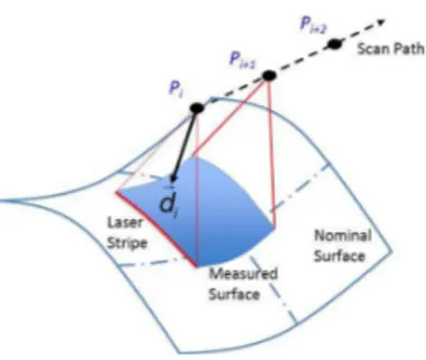
Within the context of 3D surface scanning, path planning is still a challenge to obtain a complete representation of parts in a minimum time. More generally, path planning is defined as a set of ordered points of view allowing the part digitizing without collision. Each point of view corresponds to one sensor configuration relatively to the part and allows the digitizing of one portion of the part surface. As the common objective is to minimize cycle time, the main difficulty linked to scan path planning is to define a sensor trajectory, free from collision, that leads to a good surface representation, i.e. slightly noisy and complete. This issue can be expressed as the minimization of the number of points of view while respecting quality criteria, and avoiding collisions and occlusions. A point of view
p M d
(
, )
r
is defined by a point M, and a directiond
r
, and accounts for the sensor positioning (distance and orientation) relatively to the part surface (Fig. 1).Finding the optimal path planning is an issue widely addressed in the literature, in particular for parts defined by a CAD model. Most of the methods are based on the concept of visibility. The visibility can be considered either from the part standpoint -what are the directions from which a point of the part surface is visible – or from the sensor standpoint – what is the surface area visible from the sensor point of view. Visibility is generally linked with the local normal at the point.
Fig. 1: Definition of a point of view
Tarbox and Gottschlich [9] propose to plan the path of a laser sensor by using the concept of measurability matrix. The measurability matrix results from the intersection of two matrices, one corresponding to the laser visibility the second one defining the CCD visibility. Starting from a CAD model, Xi and Shu determine optimal digitizing parameters so that the digitized surface is maximized. They split the surface into sections, each one defining a surface portion. For each section, the optimal positioning is obtained by aligning the field of view with the projected surface frontier [10]. Son et al. propose a method for path planning dedicated to a laser-plane sensor mounted on a CMM. The CAD model is first divided into functional surfaces. Each surface is thus sampled into points and corresponding normal vectors, with the objective of finding the minimum number of sensor configurations. The sampling is constrained by the size of the laser beam so that the distance between two consecutive points is less than the beam width. These two consecutive points can be digitized with the same sensor configuration if the angle between the normal vectors is less than twice the view angle of the sensor [8]. Within the context of 3D inspection Prieto et al. [5] focus on the definition of scan path planning that optimizes the quality of the point cloud collected. A point of view is considered as optimal if the view angle, defining the scanning direction, and the scanning distance lie within admissible intervals. These intervals ensure the digitizing noise to be less than the expected threshold. Their approach is specific to laser-plane sensors. Rémy [7] decomposes his method in 3 main steps: calculation of the part visibility or local visibility, calculation of the global visibility and finally calculation of the actual visibility considering both the laser beam and the CCD matrix visibility. The part surface is approximated thanks to a STL meshing whereas the space is modeled as a meshed sphere. Each vector normal of the meshed sphere defines a point of view. For each facet of the part surface S
i, the local visibility is obtained for a point of view pj if the angle between the directions of the
point of view n
j, and the local normal vector to the facet ni is less than 60°. This value ensures the
quality of the scanning. Martins et al. proposed a voxel-based approach. The CAD model is reduced into a coarse voxel-map allowing the calculation of the local normal vectors, and defining the space volume to calculate collision free trajectory. In function of the point of view accessibility, voxel can be classified as Surface, Empty or Inside [2]. The volume is divided into slices the width of which is given by the laser stripe. For each slice, a collision free scan path is generated. Consecutive paths are linked together according to a zig-zag strategy to define the final trajectory. Considering a NURBS surface Raffaeli et al. propose to subdivide the surface into portions that are included in the scanner field of view, and for which the variations of the normal vectors do not exceed a threshold. Each portion is afterwards sampled [6]. The next step of the process is point clustering. The points that can be seen from the same point of view are gathered according two conditions: the maximum of the distance between 2 points belonging to the same cluster must be less than the scanner field of view, and the maximum angle between normal vectors must remain less than 90°.
Most of the literature methods are generally well adapted for a given sensor. The method proposed in the paper is generic and suitable for any type of sensor. The approach adopts the sensor standpoint starting from the minimum number of points of view that can be defined in relation with the sensor field of view and the part dimensions. This leads to the part modeling as a voxel-map wherein the voxel size is given by the sensor field of view. The analysis thus consists in finding
2 VOXEL-BASED PATH PLANNING
The originality of the method is that it is generic for different types of digitizing sensors. For this purpose, each sensor is modeled as cone with regard to its field of view as displayed in Fig. 2.
Fig. 2: Sensor modeling in function of the sensor Field of View (FOV)
The cone axis defines the direction of the point of view, its basis corresponds to the dimensions of the field of view, and its height is given by the optimal digitizing distance. As scan path planning aims at minimizing the number of points of view leading to the complete part digitizing, the interest of the proposed approach lies in initializing the search process by considering a reduced number of points of view allowing the entire digitizing of the bounding part volume. This reduced number of points of view is defined in relation with the size of the sensor Field of View (FOV) and the part dimensions (Fig. 3).
Fig. 3: Representation of the initial set of viewpoints
The initial directions are first selected along the X, Y, Z-axes of the space. This initial set of viewpoints is equivalent to the part modeling as a voxel-map for which the voxel size (L
the size of the sensor FOV (Fig. 3). Visibility analysis is performed from this modeling. Before giving details of the approach, a series of definitions is required.
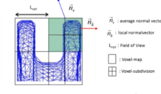
2.1 Normal vector to the voxel
A voxel is 3D pixel, most generally a cuboid. The representation of a digitized cloud of points as a voxel-map allows the identification of empty or surface voxels. In this paper, the concept of voxel-space introduced in [3] is adopted. Therefore it is possible to attach attributes, such as the normal or the barycenter, to each voxel in function of the surface portion included inside.
As the CAD model is known, it is easy to retrieve the STL representation of the surface. A surface voxel includes a portion of the object surface that means a discrete number of facets. The vector normal is defined considering the mean value of the normal vectors to each facet included in the voxel (Fig. 4): 1 1
.
.
N k k k v N k k kS n
n
S n
= ==
∑
∑
r
r
r
(2.1) where,n
vr
is the vector normal to the considred voxe, kn
r
is the vector normal to the facet k included within the voxel,S
kis the facet area, and N is the nimber of facets included in the voxeL. As the vectornormal will be sensitive to the number of facets included into the voxel, the normal vector must be assessed to check if it is representative or not of the surface portion that is included into the voxel. For this purpose, the vector normal consistency is checked as proposed in the next section.
2.2 Consistency analysis
The normal vector previously calculated is afterwards used to describe the surface portion included in the voxel. To ensure that this vector is representative of the surface in terms of visibility, a consistency analysis is performed. Actually, the surface portion may present some abrupt local curvature variations, that means normal variations non coherent with the mean value, and thus with the visibility evaluation (Fig. 4).
Fig. 4: Consistency analysis
The consistency analysis is performed considering the consistency between each local normal vector normal to the mean normal vector normal. Let us consider a facet k. If
n
kr
represents its localnormal vector, the angle
θ
k between the mean normal and the local normal can be defined as follows:.
cos
.
k v k k vn n
arc
n n
θ
=
r r
r r
(2.2)Consistency is assessed if:
k threshold
chosen equal to a quarter of the angle defining this cone.
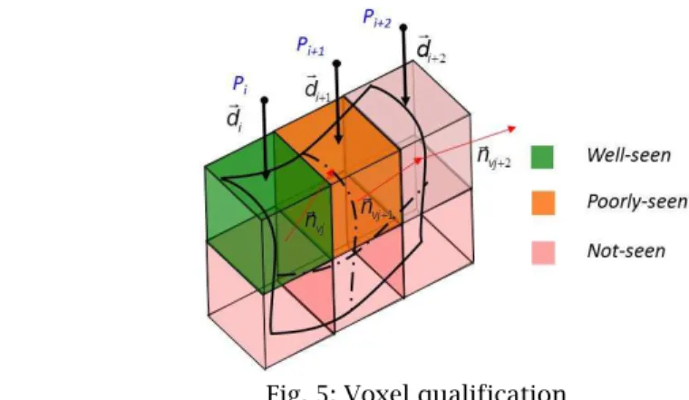
2.3 Voxel qualification
A voxel V will be said seen from a point of view
p M d
(
, )
r
if it is the first voxel intercepted by the line issued from M and directed alongd
r
(Fig. 3). Nevertheless, although a voxel is seen by a point of view, the digitizing quality cannot be reached. Indeed, numerous studies enhanced the strong influence of the view angle on the quality of the collected points. In fact, if the angle between the digitizing direction and the vector normal to the voxel is greater than a threshold, the quality of the collected points may be affected in terms of trueness or in terms of digitizing noise [4] [1]. In this direction a qualification of the seen voxels considering quality criteria is proposed.The angle between the vector normal to the voxel
n
vr
and the directiond
r
of the point of view can bedefined by:
arccos
v vd n
d n
ϕ
⋅
=
⋅
r r
r r
(2.4)Let us consider, the admissible view angle with regard to the quality expected [1] voxels are qualified as follows (Fig. 5):
!
0
≤
ϕ α
≤
adm/ 2
, the voxel is « well-seen », !/ 2
adm adm
α
≤
ϕ α
≤
, the voxel is « poorly-seen », !α
adm≤
ϕ
, the voxel is « not-seen »Fig. 5: Voxel qualification
This qualification is possible as the analysis is performed only for voxels for which the vector normal is consistent with the surface portion included.
3 METHOD DESCRIPTION: VOXEL2SCAN
The algorithm aims at defining the reduced set of points of view allowing the complete part surface digitizing with a given digitizing quality. The algorithm is initialized considering a set of initial points of view directed along the 3 principal axes of the part coordinate system, with the objective of scanning large portions of the part surface. The part is modeled as a voxel-map for which the voxel width is given by the size of the Field of View (FOV). Non digitized details are collected thanks to a
refinement of the voxel-map and by considering additional points of view. The algorithm consists of 4 main steps:
1. Definition of the voxel-map of the surface and determination of the set of initial points of view 2. Adaptive refinement of the voxel-map to ensure consistency of the normal vectors
3. Qualification of the voxels (well-seen, poorly-seen, not-seen) according to the initial set of points of view
4. Determination of additional points of view for not-seen voxels
It is important to note that a process of collision checking is done during steps 3 and 4, in order to obtain a final set of collision free points of view. The main idea here is to propose an algorithm, generic, fast and simple, that leads to a set of collision free points of view allowing the part surface digitizing within a given quality. The 4 steps are detailed in next sections.
3.1 Definition of the initial voxel-map and the initial set of points of view
The part surface to be digitized is modeled thanks to a STL meshing. This type of representation is simple enough, and allows the calculation of local properties, such as the normal vector as detailed in 2.1. The determination of the initial set of points of view is defined as follows:
- Voxelization of the part: the size of each voxel is given by the width L
opt of the FOV as
proposed in figure 2; each voxel includes a portion of the meshing that serves to calculate the normal vector according to Eqn. (2.1).
- Determination of the initial set of directions of view: the directions are chosen along the axes (X, Y, Z) that compound the coordinate system linked to the voxel-map, in both the negative and the positive directions; these 6 initial directions are chosen to simplify the first visibility analysis.
- Determination of the set of points of view: the initial voxel-map is included in a parallelepiped the faces of which are perpendicular to the 6 initial directions (Fig. 3); this parallelepiped is enlarged by a distance equal to the optimal digitizing distance D
opt, and the center of each
voxel is projected onto the nearest face of the enlarged parallelepiped defining the origin of the point of view M; the direction of the point of view
d
r
is given by the vector normal to the pane.At this stage the set of the initial points of view (M
j,
d
ir
) is defined. 3.2 Adaptive refinement
For each voxel previously defined, the consistency analysis is carried out. If the consistency is not ensured, the voxel size is divided by two, and the consistency is assessed for each one of the two new voxels. This stage is performed iteratively until the consistency is reached. Nevertheless, a shutoff parameter must be considered here to avoid too small voxel-size. Therefore, the process ends if the voxel size is equivalent to the average mesh size of the STL surface representation, even though the consistency is not reached. Each new voxel generates a new point of view as defined in the previous section (by projecting its center onto the principal nearest plane). If the vector normal is not consistent with the surface portion when the shutoff parameter is reached, the voxel is identified as “Difficult” and an orientation is proposed in function of the voxel neighborhood.
It is important to notice here that the refinement is local and well-adapted to surface portions presenting small curvature radius variations.
3.3 Qualification of the voxels
From the set of initial points of view, two different voxel lists are created in function of each voxel qualification: a list of the seen voxels L
S and a list of the LNS not-seen voxels. At the algorithm
initialization the first list is empty while the second includes all the voxels. For each direction of view
d
ir
in L
S.
2. Qualification of the seen voxels from according to the approach detailed in section 2.3; the voxels poorly-seen are removed from L
S and classified in LNS.
3. For each voxel Vj belonging to LS, the position of the point of view Mj is the offset of the center
of the voxel by a distance equal to D
opt according to the considered direction; to the voxel Vj
corresponds the point of view p
j(Mj,
d
ir
)
4. Collision checking for the point of view pj; a collision arises if a sphere, the radius of which is
given by the sensor dimensions, centered at M
j intersects at least one voxel; in this case, the
voxel V
j is removed from LS and classified in LNS
5. Selection of another direction
d
i+1r
and reiteration of the process from step 1 At this stage, to each voxel V
j belonging to LS corresponds a point of view pj.
3.4 Additional points of view
At the end of the previous step, the list L
NS may be not empty, that means that some voxels remains
not-seen or poorly-seen. Finding additional directions is thus necessary. Various methods are possible. For instance, optimized points of view could be defined by considering for each voxel the best view with regard to its vector normal. However, this could add numerous points of view that could make the trajectory planning difficult. Therefore, additional directions of view simply result from the intersection of the bisector planes of the coordinate system with third one. This solution works as for most of the sensors, half the admissible view angle α
adm/2 is greater than 45°. These directions are
added for all the voxels include in L
NS until the list becomes empty.
In the case of surfaces containing important variations of local normal vectors, the proposed algorithm may lead to a great number of voxels with small dimensions due to the refinement. The dimensions may be less than the size of the FOV. This involves that the distance between two consecutive points of view may be less than the width of the FOV. In this case, a portion of the surface may be digitized several times. To avoid this problem, the initial positions calculated from the center of the voxels of the initial voxelization are kept for these additional directions.
Once, all the points of view are determined, the sensor trajectory must be defined. As this trajectory strongly depends on not only the sensor but on the whole digitizing system used, the construction of the trajectory will not be discussed here.
4 APPLICATION
To assess the method, the previous algorithm is applied to a test surface. The surface consists of a plane, a truncated cone bonding by a spherical portion and a ruled surface. This test surface has been designed as multiple points of view are required for its complete scanning.
The method is applied to two different sensor technologies: a laser-scanner (Kreon Zephyr KZ 25) and a light-projection system (Atos – GOM) with the parameters displayed in Table 1. The choice of the admissible angle of view is given thanks to a first sensor assessment process to evaluate its quality in terms of trueness and of noise [11].
Sensor L
opt Dopt
θ
threshold αadmKZ25 20mm 145mm 60° 60°
ATOS 250 mm 490mm 60° 60°
Tab. 1. Algorithm parameters for the two sensors
Results are shown in figure 6. The refinement remains local due to the weak surface complexity. However, it is interesting to observe that the proposed method well operates regardless of the sensor technology used and provides a set of points of views ensuring the desired quality of the collected points. For both systems, the admissible angle of view is 60°. This value ensures a noise less than 3 µm
for the ATOS system and around 15 µm for the KZ25 sensor. In these conditions, the trueness can be evaluated at 3.5 µm for both digitizing systems [11]. As expected the number of points of view is reduced for the large FOV sensor.
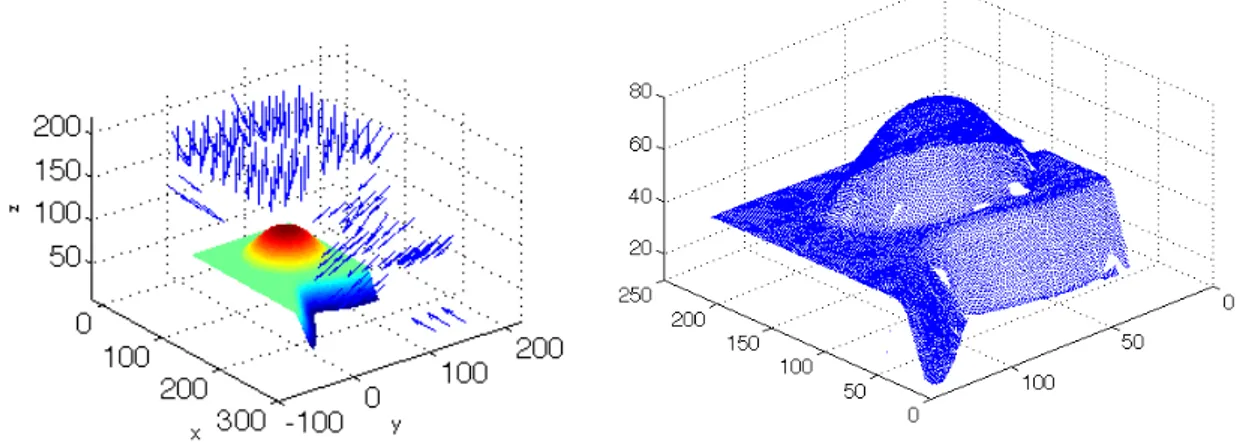
Fig. 6: Points of view for the ATOS system (left) and the KZ25 sensor (right)
The obtained point density is relatively homogeneous as overlap zones are small (Fig. 7). The comparison of the measured points with the CAD model shows that the quality obtained is also homogeneous. The main deviations are located near corner radii lie and are likely due to the machining operation. However the digitized point cloud presents digitizing holes corresponding to non-measured areas of the surface. Actually, as the model of the sensor is reduced to one point and a direction, it cannot account for the visibility of each device of the sensor (visibility laser and visibility camera). These digitizing holes illustrate one limit of the method linked with the sensor model simplicity.
Fig. 7: Result of the part digitizing with the KZ25 sensor
Nevertheless, more than 95% of the surface is measured with an expected trueness around 3.5µm and an expected noise around 15 µm. The measured surface is smaller than the nominal one: 0.024 m2
for the CAD model for 0.025 m2 for the measured one. After registration of the measured data on the
CAD model, the mean deviation is evaluated to 0.0007mm. Deviations are mainly due to machining defects near the corner radius. Some digitizing errors can be observed close to the external edge of the surface.
field of view. Starting from a reduced set of points of view admissible with regard to the field of view and the part dimensions, the algorithm checks the validity of the points of view in terms of visibility of the surface and digitizing quality. The visibility analysis relies on an adaptive voxel-map of the surface which limits significantly computational time. As illustrated through two different digitizing systems, the method applies for any type of sensors leading to the set of points of view allowing the part digitizing. The scan trajectory is afterwards defined in function of the digitizing system used. The application enhances the efficiency of the algorithm to find, with a minimum calculation effort, the set of points of view leading to the digitizing of the part surface with a given quality. The simplicity of the sensor modeling shows its limits as it does not account for the actual sensor visibility. An improvement of the method is actually in progress to account for this limit.
REFERENCES
[1] Audfray, N.; Mehdi-Souzani,C.; Lartigue C.: Assistance to automatic digitizing system selection for 3d part inspection ASME 2012 ,11th Biennial Conference on Engineering Systems Design And Analysis, ESDA2012, Nantes (France), CDRom paper N°82319, July 2-4th, 2012.
[2] Martins, F.-A.-R.; Garcıa-Bermejo, J.G.; Casanova, E.-Z.; Peran Gonzalez, J.-R.: Automated 3D surface scanning based on CAD model, Mechatronics, 15, 2005, 837–857.
[3] Mehdi-Souzani, C.; Thiebaut, F.; Lartigue, C.: Scan planning strategy for a general digitized surface, Journal of Comput. Inf. Sci. Eng., 6, 2006, 331-340.
[4] Mehdi-Souzani C.; Lartigue C.: Contact less laser-plane sensor assessment: toward a quality measurement, IDMME-Virtual Concept, 2008, Beijing, China, October 2008.
[5] Prieto, F.; Redarce, T.; Boulanger, P.; Lepage, R.: Accuracy Improvement of contactless sensor for dimensional inspection of industrial parts, International Journal of CAD/CAM - Rapid Production, 15, 2000, 345-36.
[6] Raffaeli, R.; Mengoni, M.; Germani, M.: Context dependent automatic view planning: the inspection of mechanical components, Computer-Aided Design & Applications, 10(1), 2013, 111-127.
[7] Rémy, S: Contribution à l’automatisation du processus d’acquisition de formes complexes à l’aide d’un capteur laser plan en vue de leur contrôle géométrique. PhD thesis, Université Henri Poincaré de Nancy, Juin 2004.
[8] Son, S.; Park, H.; Lee, K. H.: Automated laser scanning system for reverse engineering and inspection, International Journal of Machine Tools & Manufacture, 42, 2002, 889-897.
[9] Tarbox, G.-H.; Gottschlich, S.-N.: Planning for complete sensor coverage in inspection, Computer Vision and Image Understanding, 61(1), 1995, 84-111.
[10] Xi, F.; Shu, C.: CAD-based path planning for 3-D line laser scanning, Computer-Aided Design, 31, 1999, 473-479.
[11] Zuquete-Guarato, A.; Mehdi-Souzani, C.; Quinsat, Y.; Lartigue, C.; Sabri, L.: Towards a new concept of in-line crankshaft balancing by contact less measurement: process for selecting the best digitizing system, 11th Biennial Conference on Engineering Systems and Design Analysis, ESDA2012, Nantes (France), CDRom paper N°82166, July 2-4th 2012.