HAL Id: hal-01553457
https://hal-mines-paristech.archives-ouvertes.fr/hal-01553457
Submitted on 17 Jul 2017HAL is a multi-disciplinary open access archive for the deposit and dissemination of sci-entific research documents, whether they are pub-lished or not. The documents may come from teaching and research institutions in France or abroad, or from public or private research centers.
L’archive ouverte pluridisciplinaire HAL, est destinée au dépôt et à la diffusion de documents scientifiques de niveau recherche, publiés ou non, émanant des établissements d’enseignement et de recherche français ou étrangers, des laboratoires publics ou privés.
Excerpts from the report: “BeyondTMY
-Meteorological data sets for CSP/STE performance
simulations”
Kristian Pagh Nielsen, Frank Vignola, Lourdes Ramírez, Philippe Blanc,
Richard Meyer, Manuel Blanco
To cite this version:
Kristian Pagh Nielsen, Frank Vignola, Lourdes Ramírez, Philippe Blanc, Richard Meyer, et al.. Ex-cerpts from the report: “BeyondTMY - Meteorological data sets for CSP/STE performance simu-lations”. AIP Conference Proceedings, American Institute of Physics, 2017, SOLARPACES 2016: International Conference on Concentrating Solar Power and Chemical Energy Systems, 1850 (1), pp.140017. �10.1063/1.4984525�. �hal-01553457�
Excerpts from the Report: “BeyondTMY - Meteorological
Data Sets for CSP/STE Performance Simulations”
Kristian Pagh Nielsen
1, a), Frank Vignola
2, b), Lourdes Ramírez
3, c),
Philippe Blanc
4, d), Richard Meyer
5, e), and Manuel Blanco
6, f)1Danish Meteorological Institute, Lyngbyvej 100, DK-2100 Copenhagen, Denmark. 2Solar Radiation Monitoring Laboratory, University of Oregon, Eugene, OR 97403-1274, USA.
3CIEMAT, Avda. Complutense 40, E-28040 Madrid, Spain.
4ARMINES, 1, rue Claude Daunesse, CS10207, F-75272 Paris Cedex 06, France. 5Suntrace GmbH, Brandstwiete 46, D-20457 Hamburg, Germany.
6The Cyprus Institute, Athalassa Campus, 20 Konstantinou Kavafi Street 2121, Aglantzia, Nicosia, Cyprus. a)Corresponding author: [email protected]
b)[email protected] c)[email protected] d)[email protected]
e)[email protected] f)[email protected]
Abstract. In order to facilitate comprehensive economic modeling of CSP/STE power plants realistic long-term meteoro-logical datasets with temporal resolution down to 1 minute is a main premise. Currently available standard datasets do not fulfil this premise. The datasets also need to combine the high quality of well-maintained ground-based irradiance measurements and the global coverage of satellite-derived data. Even with the best available data it is necessary to ac-count for the uncertainty in this and the sampling uncertainty from finite time-series to enable the optimal statistical char-acterization. It is a general challenge that satellite-derived data lack the required temporal resolution, and also often does not cover periods with major volcanic eruptions. Here we see prospects in synthetically generated realistic datasets, alt-hough research and development work is required on how to optimally produce and quality assure these.
INTRODUCTION
To build a solar thermal electric (STE) power plant an investment of the order of hundreds of millions euro is needed. An investment of that size requires bank support. The banks need to have an idea of the plant production for several years into the future. A main variable here is the future variability of the meteorological conditions, where direct normal irradiance (DNI) is the primary variable of importance for concentrating solar power (CSP). This enables estimations of the project profitability (the financial gain to be expected) and the pay-back period (the time required to recover an investment) [1]. The data for financing purposes should represent as well as possible the local conditions to be expected at the plant site at least over the tenure of the loan, which typically is in the order of 15 years. Some investors interested in the ‘golden end’ of a power project might also consider up to 20-25 years. Thus, in case of CSP/STE projects: 1) The long term average of solar resources should well represent the average; 2) The interannual variability of the DNI should be represented; 3) The short-term variability of DNI, which also plays a major role on yields of CSP/STE-plants [2], should include realistic data sequences and interdependencies between the meteorological variables.
Yearly datasets of hourly solar data [3], meteorological reference years [4,5,6], typical meteorological years (TMYs) [7,8,9], all consist of 12 typical months based on a long-term (at least 10 years) meteorological data set.
These datasets have been a main data source for simulations for decades. They are, however, not optimized with respect to the DNI solar resource and they lack untypical months.
The yearly datasets also do not represent the interannual variability. To accommodate this lack, they can be sup-plemented with yearly probabilities of exceedance (PoE) values that estimate the solar resource in bad years. The PoE is the probability that a given level of yearly power generation will be exceeded. Thus P90 is the yearly produc-tion level of a system that is expected to be exceeded in 90% of all years and P99 is the yearly producproduc-tion expected to be exceeded in 99% of all years [10,11]. Consensus is needed on how to derive these PoE values. Here we show and discuss examples of the challenges in deriving them.
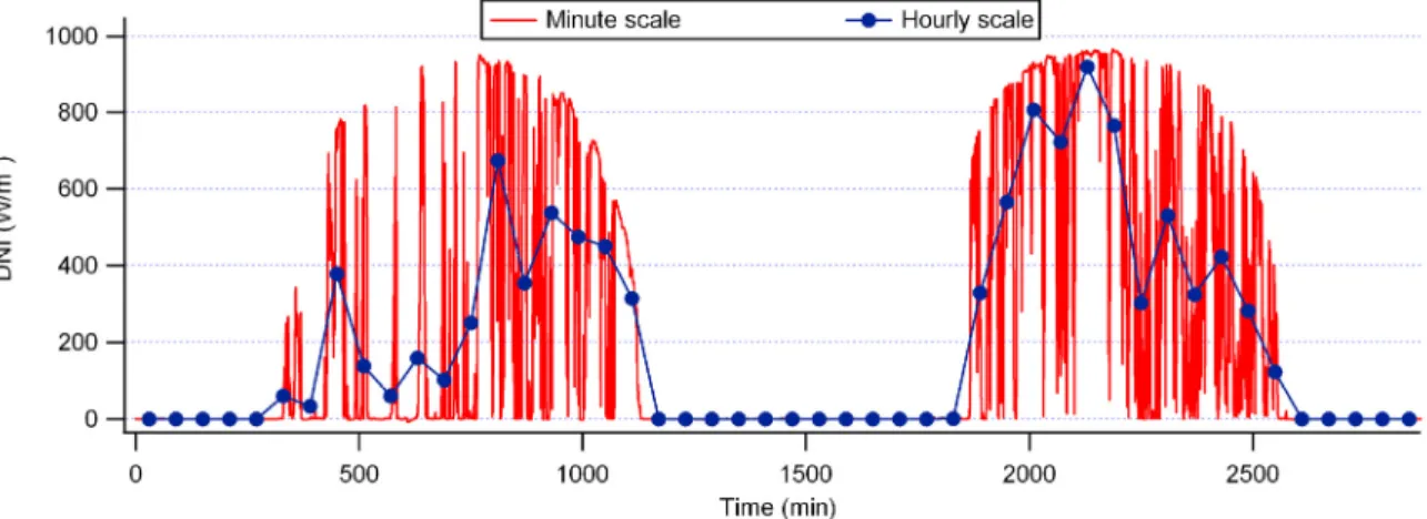
The temporal resolution in the yearly datasets is mostly 1 hour. One exception is the Design Reference Year (DRY) developed in the IEA SHC Task 9, in which DNI data with 5 minute resolution is recommended [6]. Since the short-term variability of DNI plays a major role for CSP/STE plant energy yields, optimal meteorological da-tasets should be developed that include 1 minute resolution DNI data. The difference between hourly and 1 minute resolution DNI data on two days with variable cloud cover is illustrated in Fig. 1.
FIGURE 1: Comparison of two days of DNI data on an hourly and a 1 minute scale. These measurements are from the Baseline Surface Radiation Network (BSRN) station in Carpentras, France. They have been measured with a Kipp & Zonen CH1
Pyrheli-ometer at a 1 second sampling rate averaged to 1 minute and 1 hour data [12].
In recent years, the growing number of STE projects has pushed researchers to look for solutions to specific needs of this technology. To generate TMY or reference yearly data sets several meteorological variables are weighted and compared on a monthly basis to their long term average distributions. 12 specific months are then chosen based on the fit of the weighted variables (e.g. [7,8]). Since DNI is the single most important variable for CSP/STE yield, new yearly datasets with 12 specific months chosen only from the fit of DNI have been developed [13,14]. In the ENDORSE TMY generation service [15], the maximum wind gust threshold can also be taken into account. The mirrors in a CSP/STE plant need to be placed in safe mode during strong wind gusts.
Another important development in recent years is the production of gridded data sets (e.g. [13,14]). In these sat-ellite-derived irradiances are combined with ground-based measurements to obtain global coverage that includes locations for which long-term ground-based datasets are not available. The satellite-derived irradiances need to be adapted to quality controlled ground-based measurements during at least one year and preferably two years. This process is referred to as site-adaptation [16,17] and has recently been reviewed by Polo et al. [18].
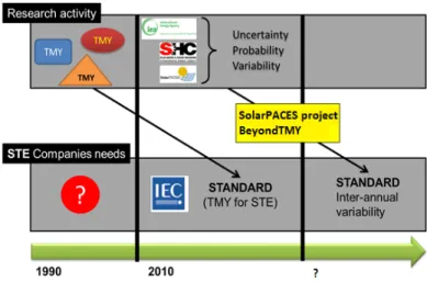
The upcoming IEC/TC117 standard for STE plants will include a technical specification (TS 62862-1-2) on yearly data set generation for STE simulations. This specification is based on several years of research, but does not include currently discussed issues such as statistical distributions, uncertainty and variability. This is because indus-trial standards are based on consensus and include only agreed minimum requirements.
FIGURE 2: Activity timeline showing the progress from research scientist methods to industrial standards.
In Fig. 2 the timeline of making such an industrial standard is illustrated. This illustrates why supplementary guidelines are needed that also include current state-of-the-art methods. The relation of the new guidelines to the current standards will be presented. For financing CSP/STE plants yearly datasets generated according to TS 62862-1-2 can be used as a base case. For detailed feasibility studies and profitability assessments additional characteriza-tions of long-term variability and uncertainty are needed. The BeyondTMY project is aimed at making ambitious recommendations in this regard form the research and development forefront.
BeyondTMY is a SolarPACES project that was started in 2015. In the project, methods for creating meteorologi-cal data sets for CSP/STE performance simulations have been reviewed, and an updated roadmap for research, de-velopment and deployment is being developed. A comprehensive report is being made in 2016. The full report will be available at the SolarPACES 2016 conference. This paper includes excerpts and our main findings from this report. We briefly describe the main data sources, the uncertainty of these, sources of DNI variability that are chal-lenging to account for, statistical characterization of long-term datasets and our outlook for the opportunities and requirements for synthetically generated datasets.
DATA SOURCES
Ground-Based Data
The most accurate DNI measurements are made with absolute cavity radiometers (ACR). The ACR DNI meas-urements are used as reference values because electrical current can be measured to a much higher degree of accura-cy than measurements of the thermal energy that other instruments measure. The internationally recognized standard for DNI is the World Radiometric Reference (WRR) developed and maintained by the World Radiation Center [19]. Periodically, other ACRs are calibrated against this standard and they achieve accuracies, at the 95% level of confi-dence, in the range of ±0.36% to 0.40% [20]. These calibrated ACRs and then used to calibrate other DNI measur-ing instruments. All certifiable calibrations of DNI measurmeasur-ing instruments can trace their calibrations to the WRR.
ACR’s are very expensive and are not intended for field operation. There are four ways to obtain DNI values from ground-based measurements in the field: 1) Field Pyrheliometers, 2) Rotating Shadowband Irradiometers, 3) Pyranometers with a shadow masks, 4) Calculations using Global Horizontal Irradiance (GHI) and Diffuse Horizon-tal Irradiance (DfHI). In most cases there are many varieties of each type of DNI instrument.
Most field pyrheliometers consist of thermopiles-based detectors at the end of a collimation tube that has a win-dow covering the aperture. The aperture and the collimation tube provide an opening with a full angle of view be-tween 5.0 and 5.7, where newer models of pyrheliometers have 5.0 full angle field of view. Note that concentrat-ing solar technologies may not utilize this exact 5.0 field of view but may utilize a narrower or broader field of view.
Other ground-based data used in meteorological datasets include: GHI measured with pyranometers, temperature and relative humidity measured in 2 meters height. Wind and wind direction measured in 10 meters height. The measurement heights are standards of the World Meteorological Organization (WMO) [21].
Satellite-Derived Data
There are a variety of ways to obtain estimates of surface solar irradiance values from satellites observations and other meteorological measurements. The basis for any modeling of solar irradiance data is the ability to accurately estimate the irradiance during cloudless periods. There are three basic ways to estimate surface irradiance from satellite images. The first is to use radiative transfer models and cloud cover information that is part of the reanaly-sis methodology used for climate studies. These are called physical models and this method has been used for the NASA/SSE irradiance database [22]. The empirical approach is based on statistical and correlation methods to model the irradiance from satellite images using ground-based measurements to determine the parameters and vali-date the model. Currently the best models use a combination of both approaches to take advantage of the physical information being gathered from satellites [18].
The 2015 IEA SHC Task 36 & 46 best practices report [22] provides a comprehensive overview of both satellite-derived and ground-based irradiance data sources.
IRRADIANCE UNCERTAINTY
All data, whether measured or modelled, is uncertain. The uncertainty is important to quantify and account for in both simulations and statistical analyses. Uncertainty should not be confused with the actual variability of the data.
To standardize the discussion of uncertainties and to set standards that provide guidelines for determining uncer-tainty and characterizing uncertainties, the Guide to Expressing Uncertainties in Measurements (GUM) was created [23]. This document explains in detail the GUM terminology and explains how to perform uncertainty analysis using the GUM procedures. The GUM model starts by defining the “measurand”, the quality that is being measured. The resulting measurement is an approximation or estimate of the measurand and a full description of the measurement includes the uncertainty of the measurement. In addition, other environment quantities that affect the measurement should be included. For example, the WRR calibrations are measurements of DNI made when DNI values >700 W/m2 under clear sky, stable weather conditions.
Traditionally, errors are viewed as having two components, a random and a systematic component. Random er-rors arrive from unpredictable or stochastic temporal and spatial variations of quantities that influence the measure-ments. Random errors can usually be reduced by increasing the number of measuremeasure-ments. The experimental stand-ard deviation is a measure of the uncertainty of the mean resulting from random effects. Systematic errors arise from a recognized effect that influences the measurements. Error has the connotation of mistake or fault while uncertainty has the connotation of ambiguity. Error and uncertainty have often been used interchangeably, but under the GUM methodology uncertainty more precisely describes the situation. The systematic effect can be quantified and if it is significant in size, an adjustment factor, also called correction factor in the literature, can be devised and applied to compensate for the effect. The uncertainty in the adjustment factor is a measure of incomplete knowledge of the value required for the adjustment. Therefore one has uncertainties in the measurements, possible adjustments made to account for some systematic effects plus the uncertainties associated with the modeled adjustments. The terms error and uncertainty should be used precisely and care should be taken to distinguish them.
The following is a sampling of possible sources of uncertainty in measurements from the GUM document. a) Incomplete definition of the measurand;
b) Imperfect reaIization of the definition of the measurand;
c) Nonrepresentative sampling — the sample measured may not represent the defined measurand; d) Inadequate knowledge of the effects of environmental conditions on the measurement or imperfect; e) Measurement of environmental conditions;
f) Personal bias in reading analogue instruments;
g) Finite instrument resolution or discrimination threshold;
h) Inexact values of measurement standards and reference materials;
i) Inexact values of constants and other parameters obtained from external sources and used in the data-reduction algorithm;
j) Approximations and assumptions incorporated in the measurement method and procedure; k) Variations in repeated observations of the measurand under apparently identical conditions.
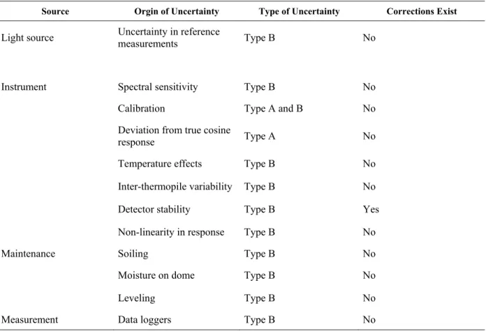
The GUM methodology breaks the uncertainties into two types: A and B. Both types are quantified by variances and/or standard deviations. The Type A evaluation is calculated from series of repeated observations For the Type B evaluations, the variance is evaluated using available knowledge, for example the characteristics of the measuring device. In the Tables 1-3 overviews of the sources of uncertainty for pyrheliometers, rotating shadowband radiome-ters and pyranomeradiome-ters with shadow masks are given, respectively.
TABLE 1. Sources of Uncertainty for Pyrheliometers.
Source Orgin of Uncertainty Type of Uncertainty Corrections Exist
Light source Uncertainty in Type B No reference measurements
Instrument Calibration Type A and B No Non-linearity of response Type A and B No Time of day Type A No Detector stability Type A Yes
Temperature effects Type A or B Exists for some instruments Maintenance Soiling Type B No
Moisture on window Type B No Tracker Alignment Type B No Measurement Data logger Type B No
TABLE 2. Sources of Uncertainty for Rotating Shadowband Radiometers.
Source Orgin of Uncertainty Type of Uncertainty Corrections Exist
Light source Uncertainty in reference measurements Type B No Instrument Spectral sensitivity Type A and B Yes
Calibration Type A and B No Deviation from true cosine
response Type A Yes Temperature effects Type A or B Yes Detector stability Type A Yes Non-linearity in response Type B No Maintenance Soiling Type B No Moisture on diffuser Type B No Leveling Type B No Measurement Data loggers Type B No
TABLE 3. Sources of Uncertainty for Pyranometers with Shadow masks.
Source Orgin of Uncertainty Type of Uncertainty Corrections Exist
Light source Uncertainty in reference measurements Type B No
Instrument Spectral sensitivity Type B No Calibration Type A and B No Deviation from true cosine
response Type A No Temperature effects Type B No Inter-thermopile variability Type B No Detector stability Type B Yes Non-linearity in response Type B No Maintenance Soiling Type B No Moisture on dome Type B No Leveling Type B No Measurement Data loggers Type B No
Further details of uncertainty characterization and discussion of the uncertainties of satellite-derived irradiances are given in the BeyondTMY report.
IRRADIANCE VARIABILITY
To be able to correctly describe the variability of DNI it is important to understand the root causes of this. Both natural and anthropogenic causes affect this variability. Several of these causes of variability are only well repre-sented in long-term meteorological dataset. A good example is the recent 2014-2016 Niño in the Pacific. An El-Niño event of similar strength last occurred in 1997-1998. The variability of this is quantified with the Multivariate El-Niño Southern Oscillation (ENSO) index (MEI) [24] or the ENSO 3.4 index that is based on Pacific sea surface temperatures and is available from the National Oceanic and Atmospheric Administration (NOAA) [25]. The ENSO is a chaotic variation that affects the cloud conditions in and around the Pacific Ocean, and in lower latitude regions around the world. For variations in the North Atlantic region the North Atlantic Oscillation (NAO) index can be used to quantify large scale variability in the tracks of extratropical cyclones over time scales of weeks and months. The cyclone tracks affect cloud occurrence and thereby the regional solar resource [26,27].
The variability of global scale volcanic eruptions poses an even greater challenge to represent due to the low fre-quency of these. Data affected by large volcanic eruptions should as the Pinatubo 1991 eruption are omitted from TMYs and other yearly datasets. Likewise, P90 and similar probability of exceedance values often are estimated with a disclaimer that major volcanic eruptions are not considered. With the latest paleoclimatic data [28], assess-ments of the major volcanic eruption variability can be made. Sulphate aerosol deposits in Antarctic and Greenland-ic Greenland-ice cores can be related to the volcanGreenland-ic sulphate aerosols that are ejected into the stratosphere. These aerosols in the stratosphere have an e-folding decay time of about 1 year [29] and thus affect the solar resource significantly. Judging from the analysis of 2500 years of paleoclimatic data [28] the likelihood of a volcanic eruption ejecting more than 0.1 aerosol optical depth (AOD) sulphate aerosols into the stratosphere within a 10-year period is 43%.
Correspondingly, the likelihoods are 22%, 7% and 1.6% for AOD larger than 0.2, 0.5 and 1.0, respectively. To put this into context, the Pinatubo 1991 eruption is estimated to have caused a maximum stratospheric AOD of almost 0.2. These estimates rely on studies of the most recent major volcanic eruptions. Since some of the past ice core sulphate deposits are biased positively by proximal high latitude volcanos, the AOD estimates are likely to be over-estimated. Work is ongoing with better isotope analysis of volcanic ice deposits that promises to enable recognition of individual volcano sources and the possibility of distinguishing tropospheric and stratospheric sulphate [30]. Thus, improved volcano risk assessments are likely to become available in the coming years.
Since the DNI resource is strongly affected by aerosols, scenarios of future trends of anthropogenic aerosol emissions are worth considering.
STATISTICAL CHARACTERIZATION OF LONG-TERM DATASETS
The long-term inter-annual DNI variability can be characterized with yearly probability of exceedance values. For example, the P90 value corresponds to the yearly DNI value that will be exceeded at least 90% of the years, during the lifetime of the project. It corresponds to complementary of the percentile: the P90 value of the yearly DNI corresponds to its 10th percentile. More generally Pxx can be used, where xx can be for instance 75% or 95%. The Pxx values depend on the statistical characterization of the yearly variability and whether the yearly data are inde-pendent and identically distributed (IID). Different Pxx values will be obtained depending on this characterization.
For illustration purpose, we have selected a very long-term (36 years; 1978-2013) and high quality in-situ meas-urements of DNI from the pyranometric station in Eugene, Oregon. This station belongs to the radiometric network UO SRML (University of Oregon Solar Radiation Monitoring Laboratory).
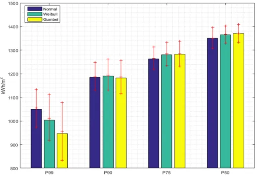
FIGURE 3: Estimations of P99, P90, P75 and P50 of the yearly DNI and the corresponding 95% confidence interval, with three fitted probability density function (PDFs), specifically the Normal, Weibull, and Gumbel PDFs.
In Fig. 3 results are shown for the PoE values P50, P75, P90 and P99 when three different statistical distributions are assumed: The Normal (or Gaussian), the Weibull, and the Gumbel distributions. Here it can be seen that the P99 estimates are more affected by which distribution is assumed than the lower PoE values.
The corresponding P90 of the yearly direct normal irradiation for the empirical data distribution is 1238 kWh/m2,
which is within the 95% confidence intervals of all P90 values for the three statistical distributions but clearly larger than these. The short-coming of deriving PoE values from empirical data distributions is that these are strongly lim-ited by the data available as noticed by Fernández Peruchena et al. [31]. The estimated statistical distributions are also limited by the available data, and by their representativeness of the actual variability. Monte Carlo simulations
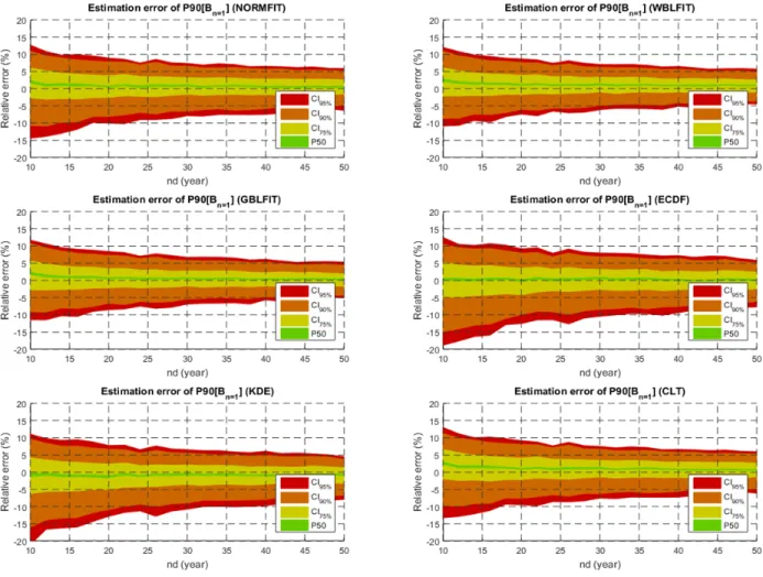
can be used to quantify the sampling uncertainty for given statistical distributions. In Fig. 4 results are shown based on 3000 Monte Carlo runs consisting of three sets of 1000 random years generated from the Normal, Weibull and Gumbell distributions, respectively.
FIGURE 4: Median errors (P50) and confidence intervals (CI) for different levels (75%, 90% and 95%) of the estimation of P90 with six tested methods: NORMFIT is the normal distribution, WBLFIT is the Weibull distribution, GBLFIT is theGumbell
distribution, ECDF is the empirical distribution, KDE is thekernel density estimation and CLT is the central limit theorem.
This illustrates how the uncertainty of the estimated P90 values depends on the length of the time series availa-ble. Nevertheless, it is important to note that this uncertainty is only “theoretical”. Firstly, the measurement uncer-tainty in the yearly DNI values should be accounted for, as this also affects the P90 estimations [32]. Secondly, this Monte-Carlo methodology is based on the very important assumption that the yearly DNI is an independent identi-cally distributed process. In the example of the yearly DNI dataset from Eugene, Oregon, this assumption is clearly questionable, and we can suspect that it is not an exception as opposed to the rule. Using statistical tools based on assumptions that are not clearly verified for their applications could be risky. There is a need of advanced statistical methodology to be able to detect and to handle non-identically distributed and/or non-independent process.
As a perspective, one can consider Monte-Carlo Markov Chain and fractional Gaussian noise random generators to be able to account for observed long-range correlation in time series [33,34,35]. These techniques of “realistic” or plausible time series generation meant to reproduce observed inter-annual correlation, trends, long-range memory (Hurst exponent) may be efficient to generate large numbers of representative synthetic very long term historical DNI dataset to be used to assess the PoE values and their related uncertainties.
OUTLOOK: CONSTRUCTION OF REALISTIC STOCHASTIC DATASETS FOR
ECONOMIC ANALYSIS
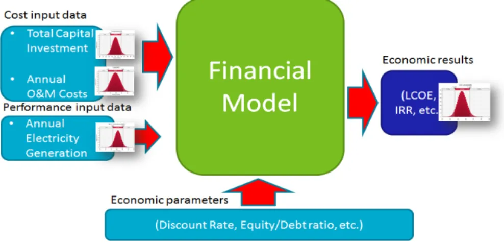
We believe that stochastic economic analysis of CSP/STE plant projects makes it possible to incorporate both the uncertainty and variability associated with the input values into the analysis to the model. Modelling of the variabil-ity of the electricvariabil-ity generation of a CSP/STE plant associated with the variabilvariabil-ity of the solar resource and the rest of meteorological variables on the site is critical. Given this and good estimates of other uncertainties, stochastic economic analysis of CSP/STE plant projects is made possible.
FIGURE 5: Stochastic economic feasibility analysis flowchart.
In Fig. 5 a flowchart of the financial modeling is shown that includes uncertainties and variability in all input da-ta. These mostly contribute to the annual electricity generation via the variability in the solar resource dada-ta. Realistic data in the sense that they reproduce the natural variability both on the 1 minute time scale and on the 100 year time scales – to include effects such as major volcanic eruptions – are needed. Since high quality measurements at these extremes of the time spectrum are not available, realistic synthetically generated data should be a main focus for future investigations.
ACKNOWLEDGEMENTS
We acknowledge support from SolarPACES for travel expenses during the BeyondTMY project. Additional funding from the Energy Development and Demonstration Program (EUDP) of the Danish Energy Agency, The Energy Trust of Oregon, The National Renewable Energy Laboratory, and Bonneville Power Administration is also acknowledged.
REFERENCES
1. M. Varela, L. Ramírez, L. Mora and M. Sidrach de Cardona, Int. J. Energ. Res. 28, 245–255 (2004).
2. K. Chhatbar and R. Meyer, “The Influence of Meteorological Parameters on the Energy Yield of Solar Ther-mal Power Plants,” 2011.
3. R. F. Benseman and F. W. Cook, New Zeal. J. Sci. 12, 698–708 (1969).
4. B. Andersen, S. Eidorff, H. Lund, E. Pedersen, S. Rosenørn and O. Valbjørn, ”Referenceåret - Vejrdata for VVS beregninger, (The Reference Year - Weather data for HVAC-calculations),” Report no. 89, Danish Build-ing Research Institute, Copenhagen, Denmark, 1974.
5. H. Lund, “The “Reference Year”, a set of climatic data for Environmental Engineering,” in Second Symposium on the Use of Computers for Environmental Engineering Related to Building, Paris, France. p. 12, (Also pub-lished as: Report no. 32, Thermal Insulation Laboratory, Technical University of Denmark), 1974.
7. I. J. R. Hall, R. R. Prairie, H. E. Anderson and E. C. Boes, “Generation of Typical Meteorological Years for 26 SOLMET Stations,” SAND78-1601, Sandia National Laboratories, Albuquerque, NM, USA, 1978.
8. W. Marion and K. Urban, “User’s Manual for TMY2s,” National Renewable Energy Laboratory, Golden, CO, USA, 1995.
9. S. Wilcox and W. Marion, “User’s Manual for TMY3 Data Sets,” NREL/TP-581-43156, National Renew-able Energy Laboratory, Golden, CO, USA, 2008.
10. F. Vignola, A. McMahan and C. Grover, “Statistical Analysis of a Solar-Radiation Dataset: Characteristics and Requirements for P50, P90, and P99 Evaluation,” in Solar Energy Forecasting and Resource Assessment, edit-ed by J. Kleissl (Elsevier, Amsterdam, The Netherlands, 2013), pp. 81–95.
11. T. Cebecauer and M. Suri, Energy Procedia 69, 1958–1969 (2015).
12. Fernández-Peruchena, C. M., M. Blanco and A. Bernardos, “Generation of series of high frequency DNI years consistent with annual and monthly long-term averages using measured DNI data,” Energy Procedia 49, 2321-2329 (2014).
13. C. Hoyer-Klick, F. Hustig, M. Schwandt and R. Meyer, “Characteristic meteorological years from ground and satellite data.” in Proceedings of the SolarPACES Conference (Berlin, Germany), 2009.
14. A. Habte, A. Lopez, M. Sengupta and S. Wilcox, “Temporal and Spatial Comparison of Gridded TMY, TDY, and TGY Data Sets,” NREL/TP-5D00-60886, National Renewable Energy Laboratory, Golden, CO, USA, 2014.
15. B. Espinar, P. Blanc and L. Wald, “Report on the Product S4: ‘TMY for production’”, Deliverable D404.1, in: EU FP7 Project ENDORSE, 2012.
16. R. Meyer, H. G. Beyer, J. Fanslau, N. Geuder, A. Hammer, T. Hirsch, C. Hoyer-Klick, N. Schmidt and M. Schwandt, “Towards Standardization of CSP Yield Assessments,” in: Proceedings of the SolarPACES Confer-ence (Berlin, Germany), 2009.
17. L. Ramírez, B. Barnechea, A. Bernardos, B. Bolinaga, M. Cony, S. Moreno, R. Orive, J. Polo, C. Redondo, I. B. Salbidegoitia, L. Serrano, J. Tovar and L. F. Zarzalejo, “Towards the standardization of procedures for solar radiation data series generation,” in: Proceedings of the SolarPACES Conference (Marrakech, Morocco), 2012. 18. J. Polo, S. Wilbert, J. A. Ruiz-Arias, R. Meyer, C. Gueymard, M. Šúri, L. Martín, T. Mieslinger, P. Blanc, I. Grant, J. Boland, P. Ineichen, J. Remund, R. Escobar, A. Troccoli, M. Sengupta, K. P. Nielsen, D. Renne, N. Geuder and T. Cebecauer, Solar Energy 132, 25-37, (2016).
19. Finsterle, W., “WMO International Pyrheliometer Comparison, IPC-XI: final report,” WMO IOM Report No. 108, (World Meteorological Organization, Geneva, Switzerland), 2011.
20. I. Reda, M. Dooraghi and A. Habte, “NREL Pyrheliometer Comparisons,” NREL/TP-3B10-63050 in Best Practices Handbook for the Collection and Use of Solar Resource Data for Solar Energy Applications Edited by M. Sengupta, A. Habte, S. Kurtz, A. Dobos, S. Wilbert, E. Lorenz, T. Stoffel, D. Renné, C. Gueymard, D. Myers, S. Wilcox, P. Blanc and R. Perez, Technical Report NREL/TP-5D00-63112, 2015.
21. WMO, “Guide to Meteorological Instruments and Methods of Observation,” WMO-No. 8, (World Meteorolog-ical Institute, Geneva, Switzerland), 2010.
22. M. Sengupta, A. Habte, S. Kurtz, A. Dobos, S. Wilbert, E. Lorenz, T. Stoffel, D. Renné, C. Guymard, D. My-ers, S. Wilcox, P. Blanc and R. Perez, “Best Practices Handbook for the Collection and Use of Solar Resource Data for Solar Energy Applications,” NREL/TP-5D00-63112, National Re-newable Energy Laboratory, Gold-en, CO, USA, 2015.
23. ISO/IEC, “ISO/IEC Guide 98-3: Uncertainty of measurement - Part 3: Guide to the expression of uncertainty in measurement (GUM:1995),” 2008.
24. NOAA, “Earth System Research Laboratory: Multivariate ENSO Index (MEI),” http://www.aoml.noaa.gov/phod/regsatprod/enso/enso34/index.php, (accessed December 2015), National Oce-anic and Atmospheric Administration, Washington, DC 20230, USA, 2015.
25. NOAA, “Physical Oceanography Division (PHOD) of AOML: El-Niño Southern Oscillation ENSO 3.4,” http://www.esrl.noaa.gov/psd/enso/mei/, (accessed November 2015), National Oceanic and Atmospheric Ad-ministration, Washington, DC 20230, USA, 2015.
26. D. Pozo-Vázquez, J. Tovar-Pescador, S. R. Gámiz-Fortis, M. J. Esteban-Parra and Y. Castro-Díez, Geophys. Res. Lett. 31, L05201 (2004).
27. M. Chiacchio and M. Wild, J. Geophys. Res. 115, D00D22 (2010).
28. M. Sigl, M. Winstrup, J. R. McConnell, K. C. Welten, G. Plunkett, F. Ludlow, U. Büntgen, M. Caffee, N. Chellman, D. Dahl-Jensen, H. Fischer, S. Kipfstuhl, C. Kostick, O. J. Maselli, F. Mekhaldi, R. lvaney, R.
Mus-cheler, D. R. Pasteris, J. R. Pilcher, M. Salzer, S. Schüpbach, J. P. Steffensen, B. M. Vinther and T. E. Wood-ruff, Nature 523 (7562), 543-549 (2015).
29. T. Crowley and M. Unterman, Earth Syst. Sci. Data Discuss. 5, 1-28 (2012).
30. M. Toohey and M. Sigl (private communication), European Geosciences Union General Assembly, Vienna, Austria, 2016.
31. C. M. Fernández Peruchena, L. Ramírez, M. A. Silva-Pérez, V. Lara, D. Bermejo, M. Gastón, S. Moreno-Tejera, J. Pulgar, J. Liria, S. Macias, R. Gonzalez, A. Bernados, N. Castillo, B. Bolinaga, R. X. Valenzuela and L. F. Zarzalejo, Solar Energy 123, 29–39, doi:10.1016/j.solener.2015.10.051, 2016.
32. N. Röttinger, F. Remann, R. Meyer and T. Telsnig, Energy Procedia 69, 2009-2018, 2015.
33. B. Mandelbrot, Water Resources Research 7 (3), 543–553, doi:10.1029/WR007i003p00543 (1971).
34. H. E. Hurst, International Association of Scientific Hydrology. Bulletin 1 (3), 13–27, doi:10.1080/02626665609493644, 1956.
35. M. Handschy, C. St. Martin and J. K. Lundquist, “Reducing Wind Power Variability by Quantifying Geo-graphic Diversity Length Scales,” poster 27, in ICEM Conference Proceedings, (Boulder, CO, USA), 2015.