HAL Id: hal-01185883
https://hal.archives-ouvertes.fr/hal-01185883
Submitted on 14 Nov 2019
HAL is a multi-disciplinary open access
archive for the deposit and dissemination of
sci-entific research documents, whether they are
pub-lished or not. The documents may come from
teaching and research institutions in France or
abroad, or from public or private research centers.
L’archive ouverte pluridisciplinaire HAL, est
destinée au dépôt et à la diffusion de documents
scientifiques de niveau recherche, publiés ou non,
émanant des établissements d’enseignement et de
recherche français ou étrangers, des laboratoires
publics ou privés.
A 2D autocorrelation method for assessing mixture
homogeneity as applied to bipolar plates in fuel cell
technology
Claire Mayer, Cendrine Gatumel, Henri Berthiaux
To cite this version:
Claire Mayer, Cendrine Gatumel, Henri Berthiaux. A 2D autocorrelation method for assessing
mix-ture homogeneity as applied to bipolar plates in fuel cell technology. Advanced Powder Technology,
Elsevier, 2011, 22 (2), pp.167-173. �10.1016/j.apt.2010.09.005�. �hal-01185883�
A 2D autocorrelation method for assessing mixture homogeneity as applied
to bipolar plates in fuel cell technology
C. Mayer-Laigle, C. Gatumel, H. Berthiaux
⇑RAPSODEE Centre, Ecole des Mines d’Albi-Carmaux, Campus Jarlard, Route de Teillet, 81000 ALBI, France
Keywords:
Intensity of segregation Scale of segregation Bipolar plate Fuel cell technology Moran’s index
a b s t r a c t
This paper presents a methodology based on spatial autocorrelation function for assessing homogeneity of a mixture and more particularly for determining the size and the number of defects in the bulk of a mixture or materials. Intensity and scale of segregation are used as conceptual tools for assessing mixture homogeneity, and have been specially adapted for this particular case. Their performances are investi-gated for detecting defects in a product manufactured from a dry powder mixture, a bipolar plate used in fuel cell technology, through a simulation of the product on Matlab (92).
1. Introduction
Assessing mixture homogeneity is a key issue in many indus-tries involved in solids processing. The general heterogeneity of a mixture is known to have an influence on the taste of a food prod-uct or the bioavailability of a drug. Several criteria based on the variance of composition of samples have been derived to access to a macroscopic quality standard which is used in the industry to accept or reject a mixture. This also results in dramatic costs in-crease, especially in the pharmaceutical industry in which recy-cling is not allowed. But even if this global criteria is satisfied, the presence of punctual defects in the mixture can drive to a lack of processability and to a loss of quality of the final product. Such a ‘‘hot point” can affect dramatically the mechanical resistance of a piece of material made of concrete, or change the visual apprecia-tion of a food product. This is also the case in the field of bipolar plate manufacturing, in which mechanical, electrical and thermal characteristics of the plates are key properties to guarantee.
Fuel cells convert chemical energy into ‘‘clean” electrical energy from hydrogen and oxygen, the only wasted product being clean water. They consist in a stack of individual cells (Fig. 1). Bipolar plates interconnect individual cells and provide connections to the outside. Their roles are to conduct electricity, keep the reaction gases separated, and channel away waste water and heat from the reaction. However, the widespread adoption of fuel cells is limited by the cost of key components as bipolar plates. The manufacture
of efficient, reliable and low cost bipolar plates is now a crucial economic issue to allow implementation of fuel cells in industrial and domestic applications. Bipolar plates may be prepared by ther-mosetting of dry powder mixtures consisting of graphite, epoxy re-sin, as well as some minor additives. The formation of polymer aggregates is sometimes observed during the mixing step. These aggregates are known to lead to mechanical deficiencies of the plates, which may cause their rupture during the demolding step. Determination of the size and number of polymer aggregates in a plate could therefore help to define better criteria for their acceptability.
In a first approach, it might seem indicated to link the detection of defects on the surface of a materials or a mixture to image anal-ysis. However, defects can be located in the bulk material, mixture or plate and may therefore not be visible, making image analysis of disputable use. The purpose of this work is to develop a methodol-ogy which can be applied regardless of the analytical method used in the measurement of sample’s composition. We will focus on the methodological tools developed to study powder mixture homoge-neity and then we will present an extension aiming at detecting defects in a bipolar plate.
2. Mixture homogeneity
The first definition for assessing homogeneity of mixtures was introduced by Danckwerts in 1952 [1]. He suggested the use of two concepts: the intensity and the scale of segregation. The first ⇑ Corresponding author.
one studies fluctuations among sample’s compositions, while the second one describes the state of subdivision of clusters.
Let us consider a mixture made of two components (A and B) being divided into N samples of a certain size. Let a and b be the mean composition of the mixture in component A and B, respec-tively, and
r
a andr
b the corresponding standard deviations. InDanckwert’s definition, the intensity of segregation is calculated as: I ¼
r
2a ab¼r
2 b ab ð1ÞA decrease of segregation intensity reflects the fact that the composition of each sample is close to the mean composition of the mixture. Instead of the definition proposed by Danckwerts, it is usual to consider the coefficient of variation, which varies in the same way as the variance but may be less dependent on the mean. CV could be used for a mixture of more than two compo-nents. Let us consider a mixture cutted into N samples, for which a key component has been defined. Let xi be the composition in
key component in sample i and x the mean composition in the samples. The CV of the mixture over the N samples reads:
CV ¼ ffiffiffiffiffiffiffiffiffiffiffiffiffiffiffiffiffiffiffiffiffiffiffiffiffiffiffiffiffiffi 1 N$P N i¼1ðxi% xÞ 2 s x ð2Þ
Indexes have been developed, based on the comparison of the standard deviation of the mixture with those of limit cases (ran-dom mixture, totally segregated mixture) but none allows to reach a better definition of the mixing homogeneity. Poux et al.[2]made a summary of the different indexes and Fan and Wang[3]reported a comparison between some indexes.
The intensity of segregation qualifies the state of macromixing
[4]. It gives no information about the structure of a mixture. In
Fig. 2, four different mixtures are represented. Each of them has the same CV but their structures are completely different. It may
happen that they could also drive to different end-used properties. To describe this, Danckwert suggested the use of a second concept, the scale of segregation. This tool provides information about the shape and the size of agglomerated particles and could therefore be linked to the size of defects.
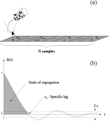
The autocorrelation function, R(r), among composition xi of N
consecutive samples, is applied to determine its numerical value by analogy to the scale of turbulence used in the statistical theory of turbulence. RðrÞ ¼ P N% r i¼1ðxi% xÞðxiþ r% xÞ PN i¼1ðxi% xÞ 2
ris the distance between two samples ð3Þ
In the associated autocorrelogram (seeFig. 3),
e
corresponds to the limit beyond which R(r) may be considered to be equal to zero, being r0the corresponding value of r. This results from statisticalthoughts[5]and depends on the confidence interval. For example, if a confidence interval of 95% is considered, then:
e
¼p2ffiffiffiffiN ð4ÞR(r) always lies between % 1 and +1. A high value of R(r) means a strong correlation between samples compositions separated by a ‘‘distance” equal to r. Therefore r0, also called the specific lag,
corre-sponds to the number of samples that are correlated among each other[5]. Danckwerts defined the scale of segregation, S, as the area under the curve:
S ¼Z r0
0 RðrÞ ' dr ð5Þ
Scan be approximated by the trapezoïdal method. However the determination of the autocorrelation function follows a discrete way and consequently the number of points may be too small to Fig. 1. Schematic representation of a fuel cell stack[17].
Decrease of the scale of segregation
apply this method. The values associated may lead to some major errors in calculations. This makes r0most likely used instead of S,
because its determination is easier and more precise.
Although the scale of segregation provides interesting informa-tion on the mixture’s structure, examples of its use in assessing powder mixture homogeneity are scarce. We can mention the work by Schofield[6]and, more recently, the one by Gyenis[7]. Both have linked the scale of segregation to the mixing mecha-nisms and particularly to convection through some simulations. Schofield has shown that autocorrelograms give rise to suitable in-dexes of mixedness for predominantly convective mixing mecha-nism. When diffusion becomes the limiting phenomena, the autocorrelation data are more difficult to interpret. Gyenis conclu-sions followed the same way. He proved that the correlation tech-nique assesses the degree of homogeneity and reveal the microstructure of concentration pattern, especially at the early stages of the process (i.e., convective and shear mechanism).
Very few other papers have been published on the subject. As a matter of fact, the determination of the scale of segregation (or the r0 associated) requires exhaustive sampling ideally at different
scale of scrutiny. The collection of accurate data is somewhat a te-dious task and authors[8,9]concluded that this measure is difficult to be performed for a real case, so that such a tool could not be used as a chore. However, with on-line analytical techniques, the study of a larger number of samples in a short time looks now pos-sible. Autocorrelation could therefore appear now as a viable tool for a better understanding of mixing process and mixture structure.
Danckwert’s approach is based on time series models where only one direction is used (the future is only determined by the
past and the present). Thus, the determination of autocorrelation coefficients can be done only for long thin (row) samples. For a bet-ter debet-termination of scale of segregation in space (I–e clusbet-ter shape and size) a 2D approach is needed. Schofield[6]extend this theory to a 2D and 3D approach of the mixture by averaging at a lag r, for each value of i, the different product ðxi% xÞðxiþ r% xÞ obtained in
the three directions. In the same way, but in a different field, it was used for studying the microstructure of a 3D porous media
[10,11]. It seems that a spatial approach could gain accuracy in the determination of the scale of segregation and the understand-ing of mixunderstand-ing mechanism. Closely related problems also arise in geographical or economics and some of this extensive work is sum-marised by Cliff and Ord[12].
3. Spatial autocorrelation
Spatial autocorrelation studies the correlation of a variable with itself through space. Thus if there is any systematic pattern in the spatial distribution of sample’s composition, it is said to be spa-tially autocorrelated. If nearby or neighbouring areas have compo-sition more alike, this indicates positive spatial autocorrelation. On the contrary, negative autocorrelation describes patterns in which neighbouring areas are unlike. At last, random patterns exhibit no spatial autocorrelation.
Several spatial autocorrelation indexes have been proposed. The most known and used follows Moran’s and Geary’s statistics[12]. Each index gives a specific information. Moran’s coefficients com-pare the value of a composition at a definite location with the val-ues at all other locations. Formally, it is defined as:
IðrÞ ¼ N $P i P j Wrði; jÞ $ ðxi% xÞðxj% xÞ S0ðrÞ $P i ðxi% xÞ 2 ð6Þ S0ðrÞ ¼ X i X j Wrði; jÞ ð7Þ
Geary’s coefficients are similar to Moran’s. However the interac-tion is not the cross-product of the deviainterac-tion from the mean but the deviation in intensities of each sample composition with one another. It is defined as:
CðrÞ ¼ 2 $ SN % 1 0ðrÞ " # $ P i P j Wrði; jÞ $ ðxi% xjÞ2 P j ðxj% xÞ 2 ð8Þ
As a consequence, Moran’s coefficients give a more global indi-cator whereas Geary’s coefficients are more sensitive to differences in small neighbourhoods[13]. I(r) varies in the same direction as Danckwert’s definition (between % 1 and 1).
In both definitions, the spatial dimension is introduced thanks to Wr(i,j) called contiguity or neighbouring matrices. It indicates
the proximity of two samples at the lag r. Wr(i,j) equals 1, if sample
iis neighbouring sample j to the distance r (Fig. 4). In the simplest case, two samples are neighbouring if r borders must be crossed to join them. A border is defined as a line between two samples. This means that contact points are excluded. Another option is to make Wr(i,j) a distance-based weight which is the inverse distance
be-tween locations i and j (1/dij). In this case Wr(i,j) are called weight
matrices.
4. Methods and simulation
The methodology we suggest for studying the number and size of defects inside a bulk mixture, or a finite product like a bipolar plate, is based on the coefficient of variation and Moran’s Index (using for Wr(i,j) a neighbouring matrixes). This may help in
stay-ing closer to Danckwerts’s definition of the intensity and the scale of segregation.
First, the materials studied are virtually cut into N parallelepi-ped rectangles samples according to two directions. Neighbouring matrices Wr, at different lag r, are built. Wrwill be a N $ N matrix
with each diagonal element equal to zero as a sample cannot be neighboured by himself. Then the coefficient of variation CV and the Moran’s coefficient are calculated. The autocorrelogram associ-ated to Moran’s coefficients is represented graphically and the spe-cific lag r0, such as I(r0) = 0 is determinated. A value of r0lesser than
1 indicates that there is no correlation among samples.
We study here a simulated typical bipolar plate manufactured from thermoset polymer and graphite. Let us consider its dimen-sions as being 60 cm ( 60 cm ( 0.5 mm. It can be regarded as a two dimensional array of parallelepiped rectangles called unit samples. Unit sample size should be related to the smallest scale of scrutiny that is considered. In this study, dimensions for unit samples were set at 1 mm by 1 mm and 0.5 mm for the thickness (total thickness). The bipolar plate is therefore represented by a 60 $ 60 matrix. Each element of the matrix takes the value of the composition in the key component (graphite) in the unit sample considered.
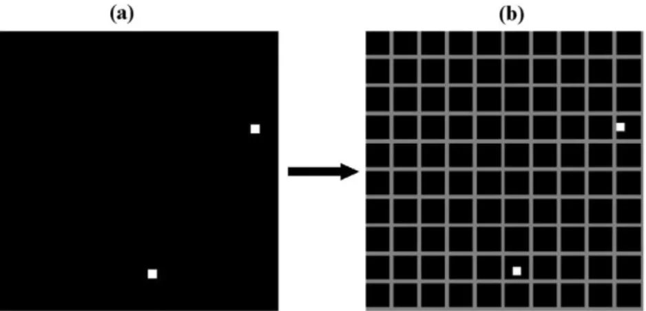
Simulation of bipolar plate composition was realised in Matlab. The plate studied had the following composition: 15% for thermo-set polymer and 85% for graphite. This composition corresponds to a real case of manufactured bipolar plate which allows to meet the requirements for thermal and electrical conductivity and mechan-ical strength of the bipolar plate. Defects were assigned to the plate with a composition in thermoset polymer equal to 100%. Number and size of defects were studied. Their locations were determined randomly. We assumed a perfect mixing state all around defects (Fig. 5a). The bipolar plate is then divided into cubic regions or samples (Fig. 5b) whose compositions are stored in a matrix. The coefficient of variation and the autocorrelation coefficients accord-ing to Moran’s model were calculated. The specific lag r0has been
determined as follows: if y(r) is a linear regression between the last value upper and the first value below the error bar, the number of correlated samples, r0, would be determined from y(r0) = 0.
5. Results and discussion 5.1. Influence of the sample size
The importance of the scale of scrutiny has been discussed in numerous articles[14–16]. The scale of scrutiny (i.e., the ‘‘best” sample size) must be defined as the final product meets the Fig. 4. Neighbouring matrix (b) for a plate (a) cut in 12 samples at the lag r = 1.
specifications it is intended for. Take the example of a powder mix-ture used to produce pharmaceutical tablets: the scale of scrutiny makes sense, it must be equal to the size of a tablet. In other field or applications, it can be more difficult to define. For a bipolar plate, specifications are of electrical, chemical, thermal and mechanical orders which makes scale of scrutiny not easy to de-fine. Regions (samples) of different sizes were therefore considered to study its influence on the coefficient of variation and the specific lag. Hereafter, cubic samples from 1 (1 by 1) to 36 (6 by 6) unit samples were considered.
Consider two bipolar plates, each containing two defects of identical size. For the first one, the defect size is set to 2 by 2 unit samples, and for the second one, the defects size is set to 3 by 3 unit samples.Fig. 6shows the evolution of CV versus sample size. It appears that increasing the sample size implies a reduction of variance. It may be noted that this variation is not linear. When the sample size (i.e., scale of scrutiny) is greater than the defect size, we observe very few changes in CV value. In fact, the CV allows to see imperfections in a mixture (or a material) whose sizes are greater than the scale of scrutiny. This means that a defect of a size smaller than that of a sample cannot be seen.
Spatial autocorrelation coefficients were calculated following Moran’s definition (Fig. 7). r0decreases with increasing sample size
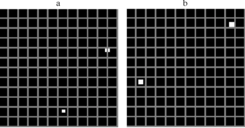
up to 1 (Fig. 8). However, the curve obtained for a defect size of 9 unit samples reach 1 faster than the curve obtained for a defect size of 4 unit samples. To explain this phenomenon, let’s have a look at the two bipolar plates that correspond to curves previously men-tioned and to their cutting into samples size of 25 unit samples (5 by 5) (Fig. 9a and b).
In this example, a defect of the size of 4 unit samples (2 by 2) is cut in two samples causing a higher r0, while defects with a larger
size (9 unit samples: 3 by 3) are each included within a single sam-ple causing a r0value less than 1. Thus, when the defect size is
low-er than that of the sample, the cutting has a strong influence on the value of r0. To investigate the influence of the defect’s size and their
number on CV and r0, only sample sizes greater than those of the
defects have been considered.
5.2. Influence of the defect size and the number of defects
Evolution of CV and specific lag r0have been studied for a
bipo-lar plate with 2 defects of different sizes (Fig. 10). Sample size is set Fig. 5. Representation of a bipolar plate obtained from Matlab simulation with 2 defects (defect size: 2 by 2 unit samples). In black: homogenized mixture; in white: thermoset polymer defects (a). Cutting of the plate (a) in 100 samples (sample size 6 by 6 unit samples) (b).
0% 5% 10% 15% 20% 25% 30% 35% 40% 45% 0 10 20 30 40
Sample size (Unit samples)
C
V
(
%)
Defect size :1 Unit samples (1 by 1) Defect size : 4 Unit samples (2 by 2) Defect size : 9 Unit samples (3 by 3)
Fig. 6. Evolution of the coefficient of variation with sample size.
0 0.2 0.4 0.6 0.8 1 1.2 0 1 2 3 4 5 6 7 8 lag r Mo ra n 's I n d ex
Sample size : 1 unit sample (1 by 1) Sample size : 4 unit samples (2 by 2) Sample size : 9 unit samples (3 by 3) Sample size : 16 unit samples (4 by 4) Sample size : 25 unit samples (5 by 5)
Fig. 7. Moran’s index obtained for a bipolar plate of defects (defect size: 2 by 2 unit samples). Different sample sizes have been considered.
0 1 2 3 4 5 6 0 5 10 15 20 25 30 35 40
Sample size (Unit samples)
R0
Defect size : 1 Unit samples (1 by 1) Defect size : 4 Unit samples (2 by 2) Defect size : 9 Unit samples (3 by 3)
to 1 unit sample. An increase of the defects size involves an in-crease of CV and specific lag. It is interesting to note that slopes seem almost parallel. This highlights the fact that an increasing de-fects size has the same impact on CV and specific lag.
For a defect size set, when the number of defects increases, the CV also increases (Fig. 11a). Conversely, the variation of r0seems to
be low (Fig. 11b). However a systematic small decrease of r0is
ob-served with the number of defects. We think that it could be linked to the fact that if the number of defects increases, they could be considered as an integral part of the plate rather than singular occurrences.
To sum up, number of defects have an influence only on CV while defects size affects both CV and specific lag. Thus defects size seems rather linked to the specific lag. Once the defect size is esti-mated, the CV could provide indications about the number of defects.
6. Concluding remarks
In this paper, we have developed a methodology for analyzing defects in 2D. This methodology allows the detection of defects in the bulk of a mixture or materials, only from samples composi-tions. It has been applied to a bipolar plate through a simulation of defects on the plate. As expected, an increase of sample size (scale of scrutiny) led to a decrease of the CV and the specific lag until the sample size is greater than those of defects. Otherwise the cutting into samples has a great influence on the value of r0. It has been
highlighted that an increase in the size of the defects implies an in-crease of the CV and r0and both follow the same profile increase. It
has also been demonstrated that if an increase of the number of de-fects involves an increase of the CV, r0remains almost constant and
is more likely related to the size of the defect. Indeed, a knowledge of these two parameters could enable the identification of defects giving ideas of their numbers and their sizes. Future work will fo-cus on investigating the effect of a non perfect mixture around the defects and the influence of the presence of defects of different sizes in the same plate.
Acknowledgements
The authors acknowledge the French National Agency for research, ANR, for his financial support through the MASCOTE project (ANR-08-MAPR-0002).
Fig. 9. Bipolar plate with two defects of size 2 by 2 unit samples (a) and two defects of size 3 by 3 unit samples (b). Cutting into samples of size 5 by 5 is shown (grey lines).
0% 10% 20% 30% 40% 50% 60% 0 5 10 15 20
Defects size (Unit samples)
CV (% ) 0 1 2 3 4 5 6 7 8 9 r0
CV
Specific lag
Defects size : 4 by 4
Defects size : 3 by 3
Defects size : 2 by 2
Defects size : 1 by 1
Fig. 10. Profile of CV and r0with increasing defects size.
0% 10% 20% 30% 40% 50% 60% 70% 80% 0 1 2 3 4 5 6
Defects size (Unit samples)
C
V
(%
)
CV for a defect size of 4 unit samples (2 by 2) CV for a defect size of 9 unit samples (3 by 3)
0 1 2 3 4 5 0 1 2 3 4 5 6
Defects size (Unit samples)
r
0Specific lag for a defect size of 4 unit samples (2 by 2) Specific lag for a defect size of 9 unit samples (3 by 3)
a
b
References
[1] P. Danckwerts, The definition, measurement and some characteristics of mixtures, Appl. Sci. Res., Sect. A 3 (1952) 279–296.
[2] M. Poux, P. Fayolle, J. Bertrand, Powder mixing: some practical rules applied to agitated systems, Powder Technol. 68 (1991) 213–234.
[3] L.T. Fan, R.H. Wang, On mixing indices, Powder Technol. 11 (1975) 27–32. [4] S. Massol-Chaudeur, H. Berthiaux, S. Muerza, et J. Dodds, A numerical model to
identify the structure of a high-dilution powder mixture, Powder Technol. 128 (2002) 131–138.
[5] C. Chatfield, The Analysis of Time Series: An Introduction, sixth ed., Chapman & Hall/CRC, London, 2003.
[6] C. Schofield, Assessing mixtures by autocorrelation, Trans. Inst. Chem. Engrs. 48 (1970) T28–T34.
[7] J. Gyenis, Assessment of mixing mechanism on the basis of concentration pattern, Chem. Eng. Process. 38 (1999) 665–674.
[8] A. Kukukova, J. Aubin, S.M. Kresta, A new definition of mixing and segregation: three dimensions of a key process variable, Chem. Eng. Res. Des. 87 (2009) 633–647.
[9] R. Hogg, Characterization of relative homogeneity in particulate mixtures, Int. J. Miner. Process. 72 (2003) 477–487.
[10] M.A. Ioannidis, M.J. Kwiecien, I. Chatzis, Statistical analysis of the porous microstructure as a method for estimating reservoir permeability, J. Petrol. Sci. Eng. 16 (1996) 251–261.
[11] H. Okabe, M.J. Blunt, Pore space reconstruction using multiple-point statistics, J. Petrol. Sci. Eng. 46 (2005) 121–137.
[12] A.D. Cliff, J.K. Ord, Spatial Processes: Models and Applications, Pion, London, 1981.
[13] M.R.T. Dale, P. Dixon, M.-J. Fortin, P. Legendre, D.E. Myers, M.S. Rosenberg, Conceptual and mathematical relationships among methods for spatial analysis, Ecography 25 (2002) 558–577.
[14] P.M.C. Lacey, Developments in the theory of particle mixing, J. Appl. Chem. 4 (1954) 257–268.
[15] N. Harnby, A comparison of the performance of industrial solids mixers using segregating materials, Powder Technol. 1 (1967) 94–102.
[16] M.H. Cooke, J. Bridgwater, The relationship between variance and sample size for mixture, Chem. Eng. Sci. 32 (1977) 1353–1357.
![Fig. 2. Representation of the scale of the segregation according to Schofield [6].](https://thumb-eu.123doks.com/thumbv2/123doknet/12231998.318464/3.892.208.672.135.395/fig-representation-scale-segregation-according-schofield.webp)