arXiv:1110.5313v1 [astro-ph.EP] 24 Oct 2011
WASP-36b: A NEW TRANSITING PLANET AROUND A METAL-POOR G-DWARF, AND AN ANALYSIS OF CORRELATED NOISE IN TRANSIT LIGHT CURVES
A. M. S. Smith1, D. R. Anderson1, A. Collier Cameron2, M. Gillon3, C. Hellier1, M. Lendl4, P. F. L. Maxted1, D. Queloz4, B. Smalley1, A. H. M. J. Triaud4, R. G. West5, S. C. C. Barros6, E. Jehin3, F. Pepe4, D. Pollacco6,
D. Segransan4, J. Southworth1, R. A. Street7, and S. Udry4 Submitted to AJ, 2011 October 24
ABSTRACT
We report the discovery, from WASP and CORALIE, of a transiting exoplanet in a 1.54-d orbit. The host star, WASP-36, is a magnitude 12.7, metal-poor G2 dwarf (Teff = 5881 ± 137 K), with
[Fe/H] = −0.31 ± 0.12. We determine the planet to have mass and radius respectively 2.27 ± 0.07 and 1.27 ± 0.03 times that of Jupiter.
We have eight partial or complete transit light curves, from four different observatories, which allows us to investigate the extent to which red noise in follow-up light curves affects the fitted system parameters. We find that the solutions obtained by analysing each of these light curves independently are consistent with our global fit to all the data, despite the apparent presence of correlated noise in at least two of the light curves.
Subject headings: planetary systems – planets and satellites: detection – planets and satellites: fun-damental parameters – stars: individual (WASP-36) – techniques: photometric
1. INTRODUCTION
Of the 171 confirmed transiting planetary systems8,
the majority have been discovered from the ground, from surveys such as WASP (Pollacco et al. 2006) and HAT-net (Bakos et al. 2004). Although the Kepler space mis-sion is discovering an increasing number of planets and even more candidate planets (e.g. Borucki et al. 2010; Borucki et al. 2011), the ground-based discoveries have the advantage that the host stars are generally brighter. This allows radial velocity measurements to measure the planetary mass, and is conducive to further characterisa-tion observacharacterisa-tions, such as measuring occultacharacterisa-tions in the infrared to probe atmospheric temperature and struc-ture.
Many of the current questions in exoplanet science are being addressed by analysing the statistical properties of the growing ensemble of well characterised transiting planetary systems. Here we report the discovery of a transiting planet orbiting the V ∼ 12.7 star WASP-36 (= 2MASS J08461929-0801370) in the constellation Hydra.
2. OBSERVATIONS 2.1. WASP photometry
1Astrophysics Group, Lennard-Jones Laboratories, Keele University, Keele, Staffordshire, ST5 5BG, UK
2SUPA, School of Physics & Astronomy, University of St An-drews, North Haugh, Fife, KY16 9SS, UK
3Institut d’Astrophysique et de G´eophysique, Universit´e de Li`ege, All´ee du 6 Aoˆut, 17, Bˆat. B5C, Li`ege 1, Belgium
4Observatoire de Gen`eve, Universit´e de Gen`eve, 51 Chemin des Maillettes, 1290 Sauverny, Switzerland
5Department of Physics & Astronomy, University of Leices-ter, LeicesLeices-ter, LE1 7RH, UK
6Astrophysics Research Centre, School of Mathematics & Physics, Queen’s University, University Road, Belfast, BT7 1NN, UK
7Las Cumbres Observatory, 6740 Cortona Drive Suite 102, Goleta, CA 93117, USA
8http://www.exoplanet.eu, 2011 October 13
36 was observed in 2009 and 2010 by WASP-South, which is located at SAAO, near Sutherland in South Africa, and by SuperWASP at the Observato-rio del Roque de los Muchachos on La Palma, Spain. The instruments consist of eight Canon 200mm f/1.8 lenses, each equipped with an Andor 2048 × 2048 e2v CCD camera, on a single robotic mount. Further de-tails of the instrument, survey and data reduction pro-cedures are described in Pollacco et al. (2006) and de-tails of the candidate selection procedure can be found in Collier Cameron et al. (2007) and Pollacco et al. (2008). A total of 13781 measurements of WASP-36 were made between 2009 January 14 and 2010 April 21.
WASP-South 2009 data revealed the presence of a transit-like signal with a period of ∼ 1.5 days and a depth of ∼ 15 mmag. The WASP light curve is shown folded on the best-fitting orbital period in Figure 1.
2.2. Spectroscopy
Spectroscopic observations of WASP-36 were made with the CORALIE spectrograph of the 1.2-m Euler-Swiss telescope. A total of nineteen spectra were taken between 2010 March 11 and 2011 January 11, and pro-cessed using the standard CORALIE data reduction pipeline (Baranne et al. 1996). The resulting radial ve-locity data are given in Table 1, and plotted in Figure 2. In order to rule out non-planetary causes for the radial velocity variation, such as a blended eclipsing binary sys-tem, we examined the bisector spans (e.g. Queloz et al. 2001), which exhibit no correlation with radial velocity (Figure. 2).
2.3. Follow-up photometry
We have a total of eight high-precision follow-up light curves of the transit of WASP-36b, summarised in Table 2. In each case differential aperture photometry was per-formed, using the IRAF/DAOPHOT package for TRAP-PIST and FTN data, and the ULTRACAM pipeline
TABLE 1
Radial velocity (RV) and line bisector span (BS) measurements of WASP-36 BJD–2 450 000 RV σRV BS (km s−1) (km s−1) (km s−1) 55266.6926 −12.843 0.027 0.079 55293.5807 −13.591 0.021 −0.017 55304.6409 −13.212 0.057 0.025 55305.5493 −13.423 0.025 −0.046 55306.6464 −12.847 0.025 0.014 55315.5600 −12.981 0.023 0.013 55316.5339 −13.624 0.028 −0.005 55317.5642 −12.977 0.033 −0.046 55320.4833 −12.821 0.030 −0.034 55359.4568 −13.527 0.040 0.002 55547.8347 −12.842 0.024 0.007 55561.8393 −12.866 0.026 0.003 55562.8651 −13.306 0.025 −0.018 55563.8184 −13.402 0.033 −0.070 55564.7341 −12.920 0.024 −0.011 55565.8211 −13.467 0.029 0.056 55567.8088 −12.870 0.023 0.001 55570.7984 −12.931 0.023 −0.028 55572.7427 −12.944 0.023 −0.068
(Dhillon et al. 2007; Barros et al. 2011) for the LT data, with aperture radii optimised to give the lowest RMS.
3. DETERMINATION OF SYSTEM PARAMETERS 3.1. Stellar parameters
The individual CORALIE spectra of WASP-36 were co-added to produce a single spectrum with a typical S/N of around 50:1. The standard CORALIE pipeline reduction products were used in the analysis. In order to improve the line profile fitting for equivalent width mea-surements, the spectrum was smoothed using a Gaussian of width σ = 0.05 ˚A. For v sin i determinations the un-smoothed spectrum was used.
The spectral analysis was performed using the meth-ods given in Gillon et al. (2009). The Hα line was used
to determine the effective temperature, Teff, while the Na
i D and Mg i b lines were used as surface gravity, log g, diagnostics. The parameters obtained from the analysis are listed in Table 3. The elemental abundances were de-termined from equivalent width measurements of several clean and unblended lines. A value for microturbulence, ξt, was determined from Fe i using the method of Magain
(1984). The quoted error estimates account for the un-certainties in Teff, log g and ξt, as well as for the scatter
due to measurement and atomic data uncertainties. The projected stellar rotation velocity, v sin i, was de-termined by fitting the profiles of several unblended Fe i lines. A value for macroturbulence, vmac, of 3.6 ± 0.3
km s−1 was assumed, based on the tabulation by Gray
(2008), and we used an instrumental FWHM of 0.11 ± 0.01 ˚A, determined from the telluric lines around 630 nm. A best fitting value of v sin i = 3.2 ± 1.3 km s−1
was obtained. The measured v sin i is sensitive to the adopted value of vmac. The recent work of Bruntt et al.
(2010) indicates a lower value of macroturbulence, vmac
= 2.6 ± 0.3 km s−1. Using this value, v sin i rises to 4.1
± 1.1 km s−1.
3.2. Neighbouring objects
The Two Micron All Sky Survey catalogue
(Skrutskie et al. 2006) reveals the presence of four fainter stars close on the sky to WASP-36. There is no evidence from analysis of catalogue proper motions that any of these stars are physically associated with WASP-36. The stars are separated from WASP-36 by 4′′, 9′′, 13′′and 17′′, meaning that they fall well within
the WASP photometric aperture, which has a radius of 48′′(3.5 pixels), but outside of the 1′′ CORALIE fibre.
In the absence of reliable optical catalogue magnitudes for all of these objects, it was necessary to measure their fluxes to quantify the effects of blending in the photom-etry. The fluxes were measured from images taken dur-ing the two transits observed with the 1.2-m Euler-Swiss Telescope (see Table 2). The fluxes relative to that of WASP-36 are as follows: 0.012 (object at 4′′ separation
from WASP-36), 0.00771 (9′′), 0.00558 (13′′) and 0.00827
(17′′). Using these flux ratios, we corrected the WASP
photometry to account for all four objects, and the high precision photometry to account for the object at 4′′,
which is within the photometric apertures used. The magnitude of this correction is minimal, and had no sig-nificant (≪ 1-σ) effect on the values of our best-fitting system parameters.
3.3. Planetary system parameters
CORALIE radial velocity data were combined with all our photometry and analysed simultaneously using the Markov Chain Monte Carlo (MCMC) method to deter-mine the system parameters. Linear functions of time were fitted to each light curve at each step of the MCMC, to remove systematic trends. Our implementation of this technique is described in detail in Collier Cameron et al. (2007) and Pollacco et al. (2008). The MCMC proposal parameters we use are: the epoch of mid-transit, t0; the
orbital period, P ; the transit duration, t14; the fractional
flux deficit that would be observed during transit in the absence of stellar limb-darkening, ∆F ; the transit impact parameter, b; the stellar reflex velocity semi-amplitude, K1; the stellar effective temperature, Teff; the stellar
metallicity, [Fe/H]; and√ecos ω and√esin ω, where e is the orbital eccentricity, and ω is the argument of perias-tron (Anderson et al. 2011). The stellar mass was deter-mined as part of the MCMC analysis, using an empirical fit to [Fe/H], Teff, and the stellar density, ρ∗(Enoch et al.
2010; Torres et al. 2010).
An initial MCMC fit for an eccentric orbit found e = 0.012+0.014−0.008(ω = 43+63−107degrees), with a 3-σ upper-limit to the eccentricity of 0.064, but we found this eccentric-ity is not significant. Following the F-test approach of Lucy & Sweeney (1971), we find that there is a 66 per cent probability that the apparent eccentricity could have arisen if the underlying orbit were actually circular. We therefore present here the model with a circular orbit, noting that the values of the other model parameters, and their associated uncertainties, are almost identical to those of the eccentric solution.
We tried fitting for a linear trend in the RVs with the inclusion of an additional parameter in our MCMC fit. Such a trend (such as that found in the RVs of WASP-34, Smalley et al. 2011) would be indicative of a third body in the system. The best-fitting radial acceleration is consistent with zero, indicating there is no evidence for an additional body in the system based on our RVs,
TABLE 2
Observing log for follow-up photometry
Light curve Date Telescope / instrument Band Nobs texp/s full / partial
(i) 2010 December 13 Eulera/ EulerCam Gunn r 94 120 partial
(ii) 2010 December 13 TRAPPISTb/ TRAPPISTCAM clear 756 10 partial
(iii) 2010 December 25 FTNc/ Spectral camera Pan Starrs z 176 60 full
(iv) 2011 January 02 TRAPPIST / TRAPPISTCAM I+ z 296 25 full
(v) 2011 January 05 TRAPPIST / TRAPPISTCAM clear 179 18 partial
(vi) 2011 January 08 TRAPPIST / TRAPPISTCAM clear 269 18 partial
(vii) 2011 January 15/16 LTd/ RISEe V + R 1290 9 full
(viii) 2011 January 21 Euler / EulerCam Gunn r 167 60 full
a1.2-m Euler-Swiss Telescope, La Silla, Chile
bTransiting Planets and Planetesimals Small Telescope, La Silla, Chile (Gillon et al. 2011; http://www.astro.ulg.ac.be/Sci/Trappist) cFaulkes Telescope North, Haleakala Observatory, Maui, Hawaii, USA
dLiverpool Telescope, Observatorio del Roque de los Muchachos, La Palma, Spain eRapid Imaging Search for Exoplanets camera (Steele et al. 2008; Gibson et al. 2008)
TABLE 3
Stellar parameters and abundances from analysis of CORALIE spectra.
Parameter Value Parameter Value
RA (J2000.0) 08h46m19.30s [Fe/H] −0.31 ± 0.12 Dec (J2000.0) −08◦01′ 36.7′′ [Na/H] −0.39 ± 0.09 Teff 5800 ± 150 K [Mg/H] −0.15 ± 0.10 log g(cgs) 4.5 ± 0.2 [Si/H] −0.17 ± 0.11 ξt 0.9 ± 0.2 km s−1 [Ca/H] −0.25 ± 0.14 vsin i 3.2 ± 1.3 km s−1 [Sc/H] −0.05 ± 0.09 log A(Li) 1.60 ± 0.15 [Ti/H] −0.22 ± 0.12
Sp. Type G2 [V/H] −0.24 ± 0.15
Distance 450 ± 120 pc [Cr/H] −0.24 ± 0.23
Age 1 - 5 Gy [Mn/H] −0.54 ± 0.13
Mass 0.97 ± 0.09 M⊙ [Co/H] −0.30 ± 0.18 Radius 0.92 ± 0.23 R⊙ [Ni/H] −0.36 ± 0.12 Additional identifiers for WASP-36:
USNO-B1.0 0819-0221838 2MASS J08461929-0801370 1SWASP J084619.30-080136.7
Note: The spectral type was estimated from Teff using the table of Gray (2008). The mass and radius were estimated using the Torres et al. (2010) calibration.
which span 10 months.
The system parameters derived from our best-fitting circular model are presented in Table 4. The correspond-ing transit and RV models are superimposed on our data in Figures 1 and 2.
3.4. System age
The lithium abundance of WASP-36 implies an age of 2 to 5 Gy according to Sestito & Randich (2005). The measured v sin i of WASP-36 gives an upper limit to the rotational period, Prot ≃ 15+10−5 days. This corresponds
to an upper limit on the age of ∼ 2+3−1 Gy using the
gyrochronological relation of Barnes (2007).
We searched the WASP photometry for periodic vari-ations indicative of star spots and stellar rotation, but no significant variation was detected. We place an up-per limit of 1.5 mmag at the 95 up-per cent confidence level on the amplitude of any sinusoidal variation. This null result is consistent with the low levels of stellar activity expected from a main-sequence G2 star. A lack of stel-lar activity is also indicated by the absence of calcium II H+K emission in the spectra. The uncertainties on the CaII emission index, log R′
HK are too large to allow
meaningful constraints to be placed on the system age
by using an activity - rotation relation such as that of Mamajek & Hillenbrand (2008).
In Figure 3 we plot WASP-36 alongside the stellar evo-lution tracks of Marigo et al. (2008). From this we infer an age of 6+5−3 Gy.
There is no evidence of any discrepancy between the ages derived from lithium abundance, gyrochronology and isochrone fitting. This suggests that the star has undergone little or no tidal spin-up, despite the presence of a massive planet in a close orbit.
3.5. Transit timing
We measured the times of mid-transit for each of the eight follow-up light curves, by analysing each light curve separately, without any other photometry (see Section 4.1). The times are displayed in Table 3.3, along with the differences, O −C between these times and those pre-dicted assuming a fixed epoch and period (Table 4). No significant departure from a fixed ephemeris is observed.
4. DETAILED ANALAYSIS OF FOLLOW-UP LIGHT
CURVES
Because we have several follow-up light curves of WASP-36 from different telescopes / instruments, whereas many planet discovery papers rely on only a single such light curve, we take the opportunity here to examine in detail the potential effects on the system pa-rameters of using only a single light curve.
For survey photometry with low SNR, the durations of ingress and egress are ill-defined, leading to considerable uncertainty in the transit impact parameter and hence to large uncertainties in the stellar density and planetary radius. So-called ‘follow-up’ transit light curves are gen-erally included in the analysis of new ground-based tran-siting planet discoveries, and are of significantly higher photometric precision than the light curves produced by survey instruments such as WASP. Such follow-up light curves are typically the result of observations with a 1 – 2-m class telescope, and are of critical importance to measuring precisely basic system parameters.
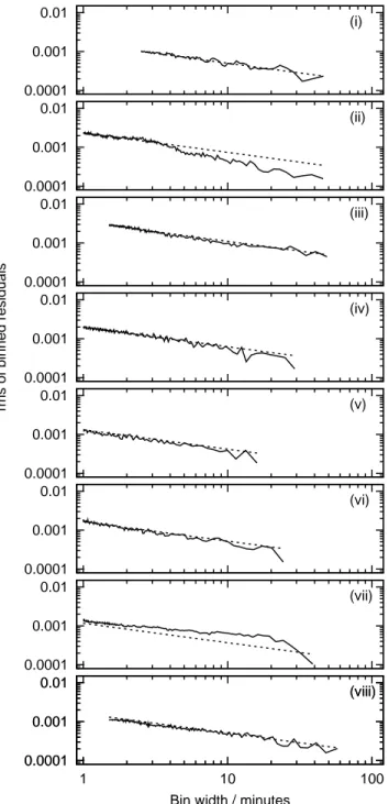
Any light curve may suffer from correlated noise, such as from observational systematics or from astrophysical sources such as stellar activity. To assess the levels of correlated noise in our follow-up light curves, we plot (Figure 4) the rms of the binned residuals to the fit of each light curve as a function of bin width, along with the white-noise expectation. For six of our light curves,
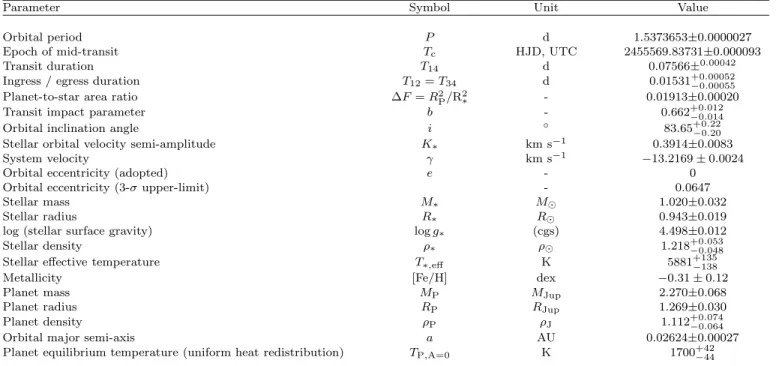
TABLE 4 System parameters
Parameter Symbol Unit Value
Orbital period P d 1.5373653±0.0000027
Epoch of mid-transit Tc HJD, UTC 2455569.83731±0.000093
Transit duration T14 d 0.07566±0.00042
Ingress / egress duration T12= T34 d 0.01531+0.00052−0.00055
Planet-to-star area ratio ∆F = R2
P/R2∗ - 0.01913±0.00020
Transit impact parameter b - 0.662+0.012−0.014
Orbital inclination angle i ◦ 83.65+0.22
−0.20
Stellar orbital velocity semi-amplitude K∗ km s−1 0.3914±0.0083
System velocity γ km s−1 −13.2169 ± 0.0024
Orbital eccentricity (adopted) e - 0
Orbital eccentricity (3-σ upper-limit) - 0.0647
Stellar mass M∗ M⊙ 1.020±0.032
Stellar radius R∗ R⊙ 0.943±0.019
log (stellar surface gravity) log g∗ (cgs) 4.498±0.012
Stellar density ρ∗ ρ⊙ 1.218+0.053−0.048
Stellar effective temperature T∗,eff K 5881+135−138
Metallicity [Fe/H] dex −0.31 ± 0.12
Planet mass MP MJup 2.270±0.068
Planet radius RP RJup 1.269±0.030
Planet density ρP ρJ 1.112+0.074−0.064
Orbital major semi-axis a AU 0.02624±0.00027
Planet equilibrium temperature (uniform heat redistribution) TP,A=0 K 1700+42−44
TABLE 5 Transit times
Light curve E TC σTC O − C
(HJD, UTC) (min) (min) (i) −17 2455543.70584 5.96 5.39 (ii) −17 2455543.70379 1.16 2.43 (iii) −9 2455556.00222 0.63 1.72 (iv) −4 2455563.68807 0.34 0.32 (v) −2 2455566.76703 8.86 6.41 (vi) 0 2455569.83686 0.86 −0.65 (vii) 5 2455577.52412 0.21 −0.02 (viii) 9 2455583.67344 0.27 −0.23 the rms of the binned residuals follows closely the white-noise expectation, indicating that little or no correlated noise is present in the data. Light curves (ii and vii) show deviation from the white-noise model, however, suggest-ing the presence of noise correlated on timescales of ∼ 1 and ∼ 10 minutes, respectively.
4.1. Method
After modelling all available data in a combined MCMC analysis (see Section 3.3), our ‘global solution’, we also ran several MCMCs each with just a single follow-up light curve in addition to the radial velocities and WASP photometry. Additionally, we re-ran each of these MCMCs applying a Gaussian prior to the stellar radius to impose a density typical of a main-sequence star (the ‘main-sequence constraint’). Such a constraint is usu-ally applied when analysing a new planet which has poor quality follow-up photometry (such as a single light curve which covers only part of the transit), and there is no evidence that the star is evolved or otherwise non-main-sequence in nature. We also performed analyses where the only photometry included was a single follow-up light curve, i.e. the WASP photometry was excluded from the analysis. The purpose of this is to determine whether
the measured depth of transit is biased by inclusion of the WASP photometry. For these runs only, the orbital period was fixed to the value determined as part of our global solution, since this parameter is very poorly con-strained by a single transit light curve and a few RVs. The epoch of mid-transit was treated as normal, and al-lowed to float freely. Finally, we performed an analysis exlcuding all follow-up photometry; the only photometry analysed was the WASP data.
4.2. Results
We produced correlation plots between several param-eters, but choose to present here only plots showing im-pact parameter against planet radius and stellar radius versus stellar mass (Figures 5 and 6, respectively). Such plots, whilst representative of the ensemble correlation plots, are particularly instructive since b and RPare two
of the major quantities we wish to measure, are largely constrained by follow-up light curves rather than by sur-vey photometry or by radial velocities, and can be signif-icantly correlated with each other, indicating a strongly degenerate solution. The stellar density is measured di-rectly from the transit light curve, and the stellar mass and radius, whilst interesting in themselves, are key in determining the values of several other system parame-ters of interest.
Several conclusions can be drawn from study of Figures 5 and 6, and similar plots, namely:
(1) each analysis including only a single follow-up light curve gives results that are consistent with our global so-lution, albeit with larger uncertainties. To measure the dispersion in the best-fitting parameter values obtained from each single follow-up light curve analysis, we cal-culated the weighted standard deviation. The standard deviations of b, RP, R∗ and M∗are 0.05, 0.08 RJup, 0.05
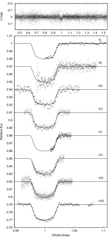
-0.2 -0.1 0 0.1 0.5 0.6 0.7 0.8 0.9 1 1.1 1.2 1.3 1.4 1.5 ∆ mag 0.76 0.77 0.78 0.79 0.8 0.81 0.82 0.83 0.84 0.85 0.86 0.87 0.88 0.89 0.9 0.91 0.92 0.93 0.94 0.95 0.96 0.97 0.98 0.99 1 1.01 0.95 1 1.05 1.1 Relative flux Orbital phase (i) (ii) (iii) (iv) (v) (vi) (vii) (viii)
Fig. 1.— Photometry. Upper panel: WASP-36 b discovery light curve folded on the orbital period of P = 1.5373653 d. For display purposes, points with an error greater than three times the median uncertainty are not shown. Lower panel: High-precision transit photometry, over-plotted with our best-fitting model (solid lines). Each individual dataset is offset in flux for clarity, and is labelled with a numeral corresponding to that in the first column of Table 2.
(2) The largest uncertainties are obtained for follow-up light curves that cover the smallest fraction of the transit (light curves i and v), as expected.
(3) The analyses which exclude the WASP photometry give larger uncertainties, but these are only significantly so when the follow-up photometry is poor. This indi-cates that the WASP photometry only makes a signifi-cant contribution to constraining the shape and depth of
-400 -300 -200 -100 0 100 200 300 400 0.5 0.75 1 1.25 1.5
Relative radial velocity / m s
-1 Orbital phase -60 -30 0 30 60 5300 5400 5500 O-C / m s -1 BJD - 2450000 -200 -100 0 100 200 -400 -300 -200 -100 0 100 200 300 400 Bis. Sp. / m s -1
Relative radial velocity / ms-1
Fig. 2.— Radial velocities. Upper panel: Phase-folded radial velocity measurements (Table 1. The centre-of-mass velocity, γ = -13.2169 km s−1, has been subtracted. The best-fitting MCMC solution is over-plotted as a solid line. Middle panel: Residuals from the radial velocity fit as a function of time. Lower panel: Bisector span measurements as a function of radial velocity. The uncertainties in the bisectors are taken to be twice the uncertainty in the radial velocities.
0.85 0.9 0.95 1 1.05 5000 5500 6000 6500 ( ρ* / ρO• ) -1/3 T*,eff / K 1.0 Gyr 12 Gyr
Fig. 3.— Modified Hertzsprung-Russell diagram. WASP-36 is plotted alongside isochrones from the evolutionary models of Marigo et al. (2008). The isochrones are for Z = 0.0093, and are regularly spaced at intervals of 1 Gy, from 1 to 12 Gy.
0.0001 0.001 0.01 (i) 0.0001 0.001 0.01 (ii) 0.0001 0.001 0.01 (iii) 0.0001 0.001 0.01 rms of binned residuals (iv) 0.0001 0.001 0.01 (v) 0.0001 0.001 0.01 (vi) 0.0001 0.001 0.01 (vii) 0.0001 0.001 0.01 (viii) 0.0001 0.001 0.01 1 10 100
Bin width / minutes
(viii)
Fig. 4.— Correlated noise in follow-up light curves – rms of binned residuals versus bin width, for light curves, 1 - 8 (solid lines). The white-noise expectation, where the rms decreases in proportion to the square root of the bin size, is indicated by the straight, dotted lines.
the transit when the follow-up light curve is incomplete. (4) Even a partial transit light curve improves the pre-cision of the measured system parameters enormously compared to those derived solely from the WASP pho-tometry and the RVs.
(5) The imposition of a main-sequence constraint does not significantly alter the parameters or uncertainties for high-precision light curves that are complete, thus indi-cating that WASP-36 is a main-sequence star. When the
follow-up light curve does not well constrain the range of possible models, however, limiting the star to the main-sequence can significantly reduce the large degeneracy in the possible solutions. This is best illustrated by light curve (iv), where the effects of the constraint are to de-crease the stellar density we find and confine the solution to a smaller area of parameter-space, close to the global solution, while largely resolving the degeneracy between b and RP.
In summary, if only one of the follow-up light curves had been available, we would have reached a solution compatible with the current best-fitting model, although the uncertainties on the model parameters may have been much greater, if the light curve was not of the highest precision. Obtaining additional light curves is clearly of benefit if one only has a light curve that par-tially covers transit. It is also useful to have multiple high-precision light curves for systems where stellar ac-tivity may bias the observed transit depth by varying amounts at different epochs, as may be the case for WASP-10b (Christian et al. 2009; Johnson et al. 2009; Dittmann et al. 2010; Maciejewski et al. 2011b,a).
5. DISCUSSION AND CONCLUSION
WASP-36 is a metal-poor, Solar mass star which is host to a transiting planet in a 1.54 d orbit. We find the planet to have a mass of 2.27 MJup, and a radius
1.27 RJup, meaning it is slightly denser than Jupiter.
There is an observed correlation between planetary ra-dius and insolation (e.g. Enoch et al. 2011), with the more bloated planets generally receiving a greater flux from their star. WASP-36b is somewhat larger than pre-dicted by the models of Bodenheimer et al. (2003), which predict radii between 1.08 (for a planet with a core at 1500 K) and 1.20 (for a core-less planet at 2000 K).
The close orbit and large radius of the planet make it a good target for measuring the planetary thermal emission, via infra-red secondary eclipse (occultation) measurements with, for example, Spitzer. The expected signal-to-noise ratios of the occultations in Spitzer chan-nels 1 (3.6 µm) and 2 (4.5 µm) are around 10 and 9 respectively.
One of the striking properties of the WASP-36 is the low stellar metallicity ([Fe/H] = −0.31 ± 0.12). Giant planets are known to be rare around such low-metallicity stars (e.g. Santos et al. 2004; Fischer & Valenti 2005), although several other low-metallicity systems are known, including the transiting systems WASP-21 ([Fe/H] = −0.46 ± 0.11, Bouchy et al. 2010), WASP-37 ([Fe/H] = −0.40 ± 0.12, Simpson et al. 2011) and HAT-P-12 ([Fe/H] = −0.29 ± 0.05, Hartman et al. 2009).
Such systems will be critical in probing our under-standing of the planet–metallicity correlation; proposed explanations for the correlation include insufficient mate-rial for proto-planetary cores to attain the critical mass needed for runaway accretion, and the suggestion that the high density of molecular hydrogen in the inner galac-tic disk is responsible for the effect (Haywood 2009). WASP-36b may also play a key role in determining whether stellar metallicity is the key parameter influenc-ing whether or not a hot Jupiter’s atmosphere exhibits a thermal inversion. Insolation was initially propounded as this parameter (Fortney et al. 2008), although this has now been largely disproved. More recently stellar
Fig. 5.— Analysis of follow-up light curves I. The MCMC posterior probability distributions for RPand b for each of the follow-up light curves. The numbering of each panel corresponds to the light curve numbering in Table 2 and the 1-σ and 2-σ contours are shown. In each case red corresponds to analysis of a single follow-up light curve plus the WASP photometry, black to the single light curve plus the WASP photometry with the main-sequence constraint imposed, and blue to that of a single light curve with no WASP photometry. The green contours indicate our global solution, and the grey contours the no follow-up photometry solution, and are therefore identical in each panel.
Fig. 6.— Analysis of follow-up light curves II. The MCMC posterior probability distributions for M∗and R∗for each of the follow-up light curves. The numbering of each panel corresponds to the light curve numbering in Table 2 and the 1-σ and 2-σ contours are shown. In each case red corresponds to analysis of a single follow-up light curve plus the WASP photometry, black to the single light curve plus the WASP photometry with the main-sequence constraint imposed, and blue to that of a single light curve with no WASP photometry. The green contours indicate our global solution, and the grey contours the no follow-up photometry solution, and are therefore identical in each panel. Also in each panel are dashed lines which are contours of constant stellar density, corresponding, from top to bottom, to 0.7, 1.0, 1.5, and 3.0 times solar density.
activity (Knutson et al. 2010) and metallicity have been advanced instead; work aiming to resolve this issue is ongoing.
6. ACKNOWLEDGMENTS
WASP-South is hosted by the South African Astro-nomical Observatory and SuperWASP by the Isaac New-ton Group and the Instituto de Astrof´ısica de Canarias; we gratefully acknowledge their ongoing support and as-sistance. Funding for WASP comes from consortium uni-versities and from the UK’s Science and Technology Fa-cilities Council (STFC). TRAPPIST is a project funded
by the Belgian Fund for Scientific Research (FNRS) with the participation of the Swiss National Science Funda-tion. MG and EJ are FNRS Research Associates. The RISE instrument mounted in the Liverpool Telescope was designed and built with resources made available from Queen’s University Belfast, Liverpool John Moores University and the University of Manchester. The Liver-pool Telescope is operated on the island of La Palma by Liverpool John Moores University in the Spanish Obser-vatorio del Roque de los Muchachos of the Instituto de Astrof´ısica de Canarias with financial support from the STFC. We thank Tom Marsh for use of the ULTRACAM pipeline.
REFERENCES Anderson, D. R., et al. 2011, ApJ, 726, L19+
Bakos, G., Noyes, R. W., Kov´acs, G., Stanek, K. Z., Sasselov, D. D., & Domsa, I. 2004, PASP, 116, 266
Baranne, A., et al. 1996, A&AS, 119, 373 Barnes, S. A. 2007, ApJ, 669, 1167
Barros, S. C. C., Pollacco, D. L., Gibson, N. P., Howarth, I. D., Keenan, F. P., Simpson, E. K., Skillen, I., & Steele, I. A. 2011, MNRAS, 416, 2593
Bodenheimer, P., Laughlin, G., & Lin, D. N. C. 2003, ApJ, 592, 555
Borucki, W. J., et al. 2010, Science, 327, 977 —. 2011, ArXiv e-prints
Bouchy, F., et al. 2010, A&A, 519, A98+ Bruntt, H., et al. 2010, MNRAS, 405, 1907 Christian, D. J., et al. 2009, MNRAS, 392, 1585 Collier Cameron, A., et al. 2007, MNRAS, 380, 1230 Dhillon, V. S., et al. 2007, MNRAS, 378, 825
Dittmann, J. A., Close, L. M., Scuderi, L. J., & Morris, M. D. 2010, ApJ, 717, 235
Enoch, B., Collier Cameron, A., Parley, N. R., & Hebb, L. 2010, A&A, 516, A33+
Enoch, B., et al. 2011, MNRAS, 410, 1631 Fischer, D. A., & Valenti, J. 2005, ApJ, 622, 1102
Fortney, J. J., Lodders, K., Marley, M. S., & Freedman, R. S. 2008, ApJ, 678, 1419
Gibson, N. P., et al. 2008, A&A, 492, 603
Gillon, M., Jehin, E., Magain, P., Chantry, V., Hutsemekers, D., Manfroid, J., Queloz, D., & Udry, S. 2011, ArXiv e-prints Gillon, M., et al. 2009, A&A, 496, 259
Gray, D. F. 2008, The Observation and Analysis of Stellar Photospheres, 3rd Edition (Cambridge University Press), p. 507
Hartman, J. D., et al. 2009, ApJ, 706, 785 Haywood, M. 2009, ApJ, 698, L1
Johnson, J. A., Winn, J. N., Cabrera, N. E., & Carter, J. A. 2009, ApJ, 692, L100
Knutson, H. A., Howard, A. W., & Isaacson, H. 2010, ApJ, 720, 1569
Lucy, L. B., & Sweeney, M. A. 1971, AJ, 76, 544
Maciejewski, G., Raetz, S., Nettelmann, N., Seeliger, M., Adam, C., Nowak, G., & Neuh¨auser, R. 2011a, A&A, 535, A7+ Maciejewski, G., et al. 2011b, MNRAS, 411, 1204
Magain, P. 1984, A&A, 134, 189
Mamajek, E. E., & Hillenbrand, L. A. 2008, ApJ, 687, 1264 Marigo, P., Girardi, L., Bressan, A., Groenewegen, M. A. T.,
Silva, L., & Granato, G. L. 2008, A&A, 482, 883 Pollacco, D., et al. 2008, MNRAS, 385, 1576 Pollacco, D. L., et al. 2006, PASP, 118, 1407 Queloz, D., et al. 2001, A&A, 379, 279
Santos, N. C., Israelian, G., & Mayor, M. 2004, A&A, 415, 1153 Sestito, P., & Randich, S. 2005, A&A, 442, 615
Simpson, E. K., et al. 2011, AJ, 141, 8 Skrutskie, M. F., et al. 2006, AJ, 131, 1163 Smalley, B., et al. 2011, A&A, 526, A130+
Steele, I. A., Bates, S. D., Gibson, N., Keenan, F., Meaburn, J., Mottram, C. J., Pollacco, D., & Todd, I. 2008, in Society of Photo-Optical Instrumentation Engineers (SPIE) Conference Series, Vol. 7014, Society of Photo-Optical Instrumentation Engineers (SPIE) Conference Series