1
About the choice of a turbulence model in building physics simulations
Mathieu Barbason1,* and Sigrid Reiter11
Université de Liège, Belgium *
Corresponding email: [email protected]
ABSTRACT
Environmental concerns and growing computer resources have promoted the emergence of new simulation tools and especially Computational Fluid Dynamics (CFD). A lot of academic studies have proved the interest of this approach. Unfortunately, for non-expert users, it is sometimes difficult to deal with turbulence modelling. Indeed, in this area, conclusions of previous studies are very fickle and sometimes contradictory. This paper aims to evaluate the impact of the turbulence modelling with different Reynolds-Average Navier-Stokes (RANS) techniques applied to airflows inside buildings. It appears that differences are often very small and completely insignificant at the design stage. However, when numerical resources requirements and computing time are considered, important differences appear in favour of the simplest model.
KEYWORDS
Building Physics Simulations, Computational Fluid Dynamics, Turbulence Modelling, Validation.
INTRODUCTION
People are more and more concerned by environmental disturbance and, for decades, the scientific community has been summoned up to make energy save in every area. Among them, building physics has developed new numerical tools – multizone and CFD simulations for example (Chen and Jiang, 1992; Heiselberg et al. 1992). In order to be of practical use, these methods need to provide accurate and reliable results in reasonable computing time and resources. As these tools become mature for academic use, they should also be usable in building physics by non-expert users.
However, flows encountered in building physics are complex and quite difficult to model. Physical phenomena are numerous: natural convection, forced convection, radiative heat transfer, etc. Among the difficulties, one can point out the choice of the turbulence model, the near-wall treatment or the discretization scheme (Chen and Jiang, 1992). This paper focuses on turbulence modelling. Comparison between different turbulence models has already been done (Voigt, 2000; Kuznik et al. 2007). Unfortunately, it has been done for specific cases and their conclusions are fickle and sometimes contradictory. This paper aims to compare three turbulence models in four different cases to have a global approach.
METHODS
Turbulence is very difficult to capture numerically due to the seemingly random behaviour of the fluid. The convective part in the Navier-Stokes equations cannot be neglected anymore. Consequently, equations become unclosed and one or two new equations are needed to describe the turbulence aspect. There are three main approaches to model turbulence in CFD: Direct Numerical Simulation (DNS), Large-Eddy Simulation (LES), RANS simulation. DNS calculates every significant turbulent phenomenon inside the flow while RANS simulation
2
modelling which permits quick simulations but has reliability drawbacks in building physics. The second one is based on two equations: one for the turbulence production – k – and one for the rate of the dissipation of turbulence – ε. This approach is the most used one in building physics. The third approach involves two equations: one for k and one for the turbulence frequency – ω. It is slower than the k-ε model but it simplifies drastically near-wall treatment because of a low Reynolds correction which exempts the model from wall functions.
For the k-ε and the k-ω models, there are different variations. These variations were studied for the present cases and differences were so small that it would not be interesting to present the results for every model. For this reason, a model was selected inside each family. For the k-ε family, it is the ReNormalization Group (RNG) k-ε model (Yakhot and Orszag, 1986) that was selected. Indeed, this model is the most used in building physics. For the k-ω family, the Shear-Stress Transport k-ω model (Menter, 1994) was selected because Kuznik and al. (2007) proved that it was the best way to simulate a jet.
In the followings, four cases were chosen such that a large range of physical phenomena are investigated: a free float case, a case of mechanical ventilation, a case of natural ventilation and a radiation case. For each case, experimental data are provided to prove the reliability of CFD in building physics numerical simulations. It will also permit to evaluate the validity of each turbulence model.
Here is a brief description of the four cases investigated:
Case 1: Free Float Case
This validation step is based on the experimental results obtain by Yuan et al. (1999). It describes the airflow in a typical office (see Figure 1.a). Despite a displacement ventilation, the flow is mainly induced by the natural convection due to thermal loads. The main difficulty lies in the very small forces in stakes. Indeed, they induce numerical instabilities (Cook, 1997). It should be noted that obstacles inside the room represent also a challenge for modelling.
Case 2: Mechanical Ventilation Case
The second studied case comes from a French study (Kuznik et al. 2007). It is a very basic case without obstacle in the room (see Figure 1.b). The convection cell is this time created exclusively by the mechanical ventilation. Moreover, jet modelling has always been a difficult point of airflow simulations. It will be approached thanks to this case.
3
a) b)
Figure 1. Illustrations of the cases. a) Free Float Case (Yuan et al. 1999), b) Mechanical Ventilation Case (Kuznik et al. 2007).
Case 3: Natural Ventilation Case
This case was first studied by Jiang and Chen (2003). There are two types of natural ventilation: buoyancy-driven and wind-driven ventilation. The first case was retained because it is the most difficult to model. Buoyancy-driven ventilation is also the most interesting case in temperate climate. Indeed, the “worst scenario” for indoor air quality that could happen is a warm and windless day (Jiang et al., 2004).
The chosen case is a test room inside a bigger room which simulates external conditions. A window permits air changes inside the test room (see Figure 2.a for the test room). This case is the occasion to understand deeply turbulence modelling thanks to the turbulence statistical analysis that was realized by the original authors.
Case 4: Radiation Case
Eventually, this case permits to the operator to deal with radiant panels (hot wall in this case). The experimental data comes from a study of the University of Liège led by Tang (1998). The test room is composed of two parts separated by an opening (see Figure 2.b). There is a heating wall in the smallest part. The main issue will be the near-wall treatment. Indeed, it influences greatly the reliability of the results.
a) b)
Figure 2. Illustrations of the cases. a) Natural Ventilation Case (Jiang and Chen, 2003), b) Radiation Case (Tang, 1998).
4
velocities, results are quite good. Indeed, due to their very small values, there is a big incertitude on air velocities measurements, but qualitatively, results are in good agreement.
Figure 3. Results of the Free Float Case.
The comparison between the three turbulence models shows that every approach is good but there is a major difference in calculation time as Table 1 indicates.
Table 1. Time comparison for the Free Float Case1
Turbulence Model Spalart-Allmaras k-ε k-ω
Computational Time 3h51 4h33 6h27
Case 2: Mechanical Ventilation Case
Results for the Mechanical Ventilation Case are shown on Figure 4. Once again, agreement is very good, especially for the k-ω turbulence model. Unfortunately, it is one more time the most expensive in computational time as Table 2 indicates. Between the two two-equations models, differences speak in favour of the k-ω even if there is a change in computing time.
1 These times do not include the elaboration of the numerical case. This can become very critical for complex
case, which is not the case for the four presented cases. This factor has to be taken into account by the operator as soon as possible.
5 Figure 4. Results of the Mechanical Ventilation Case.
Table 2. Time comparison for the Mechanical Ventilation Case
Turbulence Model Spalart-Allmaras k-ε k-ω
Computational Time 6h37 13h36 17h41
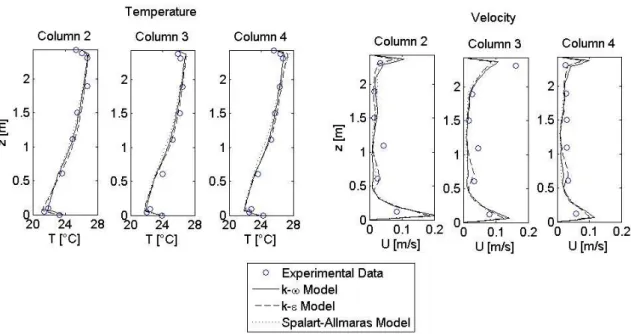
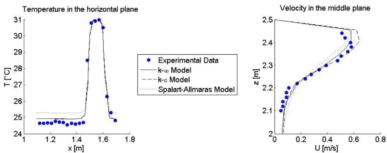
Concerning the description of the jet, Kuznik et al. studied the jet in perpendicular planes. Comparing their measurements with our simulations shows that air temperature is quite well simulated (except for the Spalart-Allmaras far away from the inlet) but air velocities show some discrepancies, especially the Spalart-Allamaras model (Figure 5). This proves once again the difficulty of jet simulation and also the limitations of a single-equation model as Spalart-Allamaras one.
Figure 5. Results in perpendicular planes
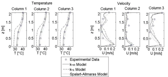
Case 3: Natural Ventilation Case
Figure 6 shows the results for the natural ventilation case. On one hand, it appears that k-ω and Spalart-Allmaras turbulence models are in good agreement with experimental data. On the other hand, the k-ε model does not give satisfactory results. This case is very complex to model because of the interaction between the two parts and the important thermal load inside the room which make that there is an important temperature gradient inside the test room. One explanation of the error made by the k-ε turbulence model could be that wall functions are not performing well near the thermal load and that it brings numerical errors.
Concerning the computing time, there is no comparison because each calculus took a lot of time and required several parameters adaptation during the calculation. So a comparison should be irrelevant, but it is likely that it is in the same proportion than the past cases.
6 Figure 6. Results of the Natural Ventilation Case.
Another interesting point to investigate is the air exchanges between the rooms. Experimental measurements indicate that there are between 6.75 and 7.92 Air Changes per Hour (ACH). Logically, the best result is obtained with the two-equations turbulence model k-ω (the k-ε model was not investigated) with a value of 7.95 ACH. So, the exchanges are slightly overestimated. The Spalart-Allmaras model gives a result of 8.15 ACH. This agreement between experimental data and numerical results is very important because air changes are crucial for occupant’s comfort.
Case 4: Radiation Case
Results of this case are drawn at Figure 7. The agreement is still quite good; the mean error is indeed less than 0.2°C for each turbulence models. One more time, there is no big differences between different turbulence models. It is interesting to see the impact of the near-wall treatment. Indeed, k-ε model is here based on wall functions. It is not the case for k-ω model, thanks to a low-Reynolds correction. So, it can be concluded that wall functions implemented in Fluent works correctly. This aspect is very important and has been discussed for years (Chen and Jiang, 1992).
7
The results for the computing time comparison remain in the same proportion than for the other cases. The Spalart-Allmaras is doing very well and the k-ω model is the slowest one to converge.
Table 3. Time comparison for the Mechanical Ventilation Case
Turbulence Model Spalart-Allmaras k-ε k-ω
Computational Time 3h05 5h51 9h53
DISCUSSIONS
Results for the four cases prove the slight impact of the turbulence model choice when several RANS techniques are used. Reliability is assured in each case (except the natural ventilation case with a k-ε turbulence model). Of course, two-equations models (k-ε and k-ω) give better results than the Spalart-Allmaras model but this improvement has a cost. So, the point is to make the best compromise.
If a project is still at a preliminary design, it seems that the choice of the turbulence model will not affect the reliability of the results. Indeed, the incertitude in the design dominates completely the lack of reliability of the Spalart-Allmaras model. However, for a final design, the operator should switch to a more complex turbulence model. If the computing time and the numerical resources are not a worry, the k-ω model should be used.
For non-expert users, the choice of the turbulence model and/or near-wall treatment is a real problem. This paper shows that a constant approach is possible for turbulence modelling. The Spalart-Allmaras is a good choice if time and resources are issues; otherwise the k-ω turbulence model is better. The choice of a k-ε model is a good compromise except for natural ventilation with important thermal loads inside the room.
This paper proves also that when several devices are used simultaneously (for example, a mechanical ventilation with an open window), the choice of the turbulence model will not affect the description of the airflow near one of the device.
Despite these observations, every user of CFD software needs a strong knowledge in numerical issues and should validate their approach. Indeed, operators have to be conscious of the limitations of the CFD. This new tool for building engineers will not replace older tools but it will help them to improve their comprehension of building physics.
CONCLUSIONS
As CFD will be more and more used, building engineers will have to deal with turbulence models in the future. This question is very important because the future of CFD use depends also on the easiness of utilization. This paper tends to prove that the choice of the turbulence model is only a matter of compromise. There is no bad approach. Results for different RANS models remain very close and every turbulence model can be validated. It would be interesting to compare these results with LES ones. Theoretically, there should be an improvement in the results.
This paper proves, if it was still necessary, that CFD is now mature for the industrial world. It will soon become essential for building engineers because of the increasing concerns in energy consumptions and indoor comfort. This software will permit huge progresses in buildings design. It will help to have a better prediction of Indoor Air Quality and Building Energy Performance. It will also permit to avoid wrong design and to improve people’s comfort.
8
Chen Q. and Jiang Z. 1992. Significant questions in predicting room air motion. ASHRAE Transactions, 98, 929-939.
Heiselberg P., Murakami S. and Roulet C.-A. 1992. Ventilation of large spaces in buildings. IEA Energy Conservation in Buildings and Community Systems, Annex 26: Energy Efficient Ventilation of Large Enclosures, 324 pages.
Jiang Y. and Chen Q. 2003. Buoyancy-driven single-sided natural ventilation in buildings with large openings. International Journal of Heat and Mass Transfer, 46, 973-988. Jiang Y., Alloca C. and Chen Q. 2004. Validation of CFD simulations for natural ventilation.
International Journal of Ventilation, 2(4), 359-370.
Kuznik F., Rusaouën G. and Brau J. 2007. Experimental and numerical study of a full scale ventilated enclosure: Comparison of four two equations closure turbulence models. Building and Environment, 42, 1043-1053.
Menter F.R. 1994. Two-equation eddy-viscosity turbulence models for engineering applications. AIAA Journal, 32(8), 1598-1605.
Spalart P. and Allmaras S. 1992. A one-equation turbulence model for aerodynamic flows. Technical report AIAA-92-0439, American Institute of Aeronautics and Astronautics. Tang D. 1998. CFD modelling and experimental validation of air flow between spaces. In:
Proceedings of the 6th International Conference on Air Distribution in Rooms – Roomvent 98, Stockholm, Vol. 2, pp. 547-554.
Voigt L.K. 2000. Comparison of turbulence models for numerical calculations of airflow in an annex 20 room. Technical Report, Danish Technical University of Lyngby.
Yakhot V. and Orszag S.A. 1986. Renormalization group analysis of turbulence: I. Basic theory. Journal of Scientific Computing, 1(1), 1-51.
Yuan X., Chen Q., Glicksman L.R., Hu Y. and Yang X. 1999. Measurements and computations of room airflow with displacement ventilation. ASHRAE Transactions, 105(1), 340-352.