Révision automatique de théories écologiques

(1)

(2)

RÉVISION AUTOMATIQUE

DE THÉORIES ÉCOLOGIQUES

par

Philippe Desjardins-Proulx

thèse présentée au Département de biologie en vue de l’obtention du grade de docteur ès sciences (Ph.D.)

FACULTÉ DES SCIENCES UNIVERSITÉ DE SHERBROOKE

(3)

Le 11 juillet 2018

le jury a accepté la thèse de Monsieur Philippe Desjardins-Proulx dans sa version finale.

Membres du jury

Professeur Dominique Gravel Directeur de recherche Département de biologie

Professeur Timothée Poisot Co-directeur de recherche Département de sciences biologiques

Université de Montréal

Professeur Pierre-Étiennes Jacques Président rapporteur

Département de biologie

Professeur Alireza Tamaddoni Nezhad Évaluateur externe

Department of Computer Science University of Surrey

Professeur Shengrui Wang Évaluateur interne Département d’informatique

(4)

(5)

(6)

(7)

SOMMAIRE

À l’origine, ce sont des difficultés en biologie évolutive qui ont motivé cette thèse. Après des décennies à tenter de trouver une théorie basée sur la sélection capable de prédire la diversité génomique, les théoriciens n’ont pas trouvé d’alternatives pratiques à la théorie neutre. Après avoir étudié la relation entre la spéciation et la diversité (Annexes A, B, C), j’ai conclu que l’approche traditionnelle pour construire des théories serait difficile à appliquer au problème de la biodiversité. Prenons par exemple le problème de la diversité génomique, la difficulté n’est pas que l’on ignore les mécanismes impliqués, mais qu’on ne réussit pas à construire de théories capable d’intégrer ces mécanismes. Les techniques en intelligence artificielle, à l’inverse, réussissent souvent à construire des modèles prédictifs efficaces justement là où les théories traditionnelles échouent. Malheureusement, les modèles bâtis par les intelligences arti-ficielles ne sont pas clairs. Un réseau de neurones peut avoir jusqu’à un milliard de paramètres. L’objectif principal de ma thèse est d’étudier des algorithmes capable de réviser les théories écologiques. L’intégration d’idées venant de différentes branches de l’écologie est une tâche difficile. Le premier défi de ma thèse est de trouver sous quelle représentation formelle les théories écologiques doivent être encodées. Contrairement aux mathématiques, nos théories sont rarement exactes. Il y a à la fois de l’incertitude dans les données que l’on collecte, et un flou dans nos théories (on ne s’attend pas à que la théorie de niche fonctionne 100% du temps). Contrairement à la physique, où un petit nombre de forces dominent la théorie, l’écologie a un très grand nombre de théories. Le deuxième défi est de trouver comment ces théories peuvent être révisées automatiquement. Ici, le but est d’avoir la clarté des théories traditionnelles et la capacité des algorithmes en intelligence artificielle de trouver de puissants modèles prédictifs à partir de données. Les tests sont faits sur des données d’interactions d’espèces.

Mots-clés : Intelligence Artificielle ; apprentissage automatique ; écologie théorique ; intérac-tion des espèces.

(8)

REMERCIEMENTS

Je tiens à remercier mes deux directeurs, Dominique Gravel et Timothée Poisot, non seulement pour leur soutien, mais surtout pour les intéressantes, passionnées et vigoureuses discussions sur la théorie et l’écologie. Ma passion en apprentissage automatique est née durant mes études et c’est au cours de nos discussion que j’ai découvert le sujet de la révision automatique de théories scientifiques. Ce doctorat n’est que le début de mes recherches sur le sujet et je vous en suis reconnaissant.

Je remercie le CRSNG (Conseil de recherches en sciences naturelles et en génie du Canada), Microsoft, et NVIDIA d’avoir financé ce doctorat.

Je remercie mes collabateurs : James Rosindell, Ignasi Bartomeus, Idaline Laigle, et aussi les membres du laboratoire, Hedvig Nenzén, Steve Vissault, Guillaume Blanchet, pour leur aide et commentaires pertinents.

Finalement, je tiens à remercier de tout coeur mes parents, Sergine Desjardins et Rodrigue Proulx, pour leur soutien indéfectible pendant toutes ces années. Je vous aime beaucoup !

(9)

(10)

TABLE DES MATIÈRES

SOMMAIRE . . . vi

REMERCIEMENTS . . . vii

LISTE DES ABBRÉVIATIONS . . . xiii

LISTE DES TABLEAUX . . . xv

LISTE DES FIGURES . . . xvii

1 INTRODUCTION GÉNÉRALE . . . 1

1.1 La grande obsession . . . 1

1.2 Interaction des espèces . . . 3

1.3 Deux questions . . . 4

1.4 Représentation des connaissances . . . 5

1.5 Apprentissage automatique . . . 5

1.6 Le plan de la thèse . . . 8

2 ECOLOGICAL SYNTHESIS AND ARTIFICIAL INTELLIGENCE . . . 9

2.1 Description de l’article et contribution . . . 9

2.2 Ecological Synthesis . . . 10

2.3 A.I. and knowledge representation . . . 11

2.4 A quick tour of knowledge representations . . . 12

2.5 Beyond monolithic systems . . . 16

2.6 Case study : The niche model . . . 17

2.7 Where’s our unreasonably effective paradigm ? . . . 21

2.8 References . . . 22

3 ECOLOGICAL INTERACTIONS AND THE NETFLIX PROBLEM . . . 27

3.2 Abstract . . . 28

3.3 Introduction . . . 28

(11)

3.4.1 Data . . . 31

3.4.2 K-nearest neighbour . . . 31

3.4.3 Supervised learning . . . 34

3.4.4 Code and Data . . . 35

3.5 Results . . . 36

3.5.1 Recommendation . . . 36

3.5.2 Supervised learning . . . 36

3.6 Discussion . . . 40

4 THE K NEAREST NEIGHBOUR ALGORITHM WITH THRESHOLD TO PREDICT ECOLOGICAL INTERACTIONS . . . 47

4.3 Methods . . . 49

4.3.1 Data . . . 49

4.3.2 Imputation with theK nearest neighbour algorithm . . . 50

4.3.3 Scoring . . . 51

4.4 Results . . . 51

4.4.1 KNN . . . 51

5 COMBINING ECOLOGICAL THEORIES WITH MACHINE LEARNING USING FUZZY LOGIC . . . 59

5.2 Abstract . . . 60 5.3 Introduction . . . 60 5.4 Method . . . 62 5.4.1 Data . . . 62 5.4.2 Measure of success . . . 64 5.4.3 Supervised learning . . . 64

5.4.4 Fuzzy knowledge base . . . 64

5.4.5 Revising theories . . . 68

(12)

5.6 Results . . . 69

6 RELATIONAL APPROACHES TO ECOLOGICAL THEORIES . . . 77

6.2 Synthesis . . . 78

6.3 Relational thinking with predicate logic . . . 80

6.3.1 Relational ? . . . 85

6.3.2 Clausal forms . . . 85

6.4 Probabilistic graphical models . . . 86

6.5 Markov logic : The union of predicate logic with probability theory . . . 90

6.6 Learning weights and theory revision in Markov logic . . . 95

6.7 Markov logic meets the Salix data-set : initial model . . . 95

6.8 Results . . . 98

7 DISCUSSION ET CONCLUSION GÉNÉRALE . . . 107

7.2 Résultats en bref . . . 107

7.2.1 Méthodes classiques . . . 107

7.2.2 La clarté par le flou . . . 108

7.2.3 Logique de Markov . . . 108

7.3 Conclusion : retour sur les deux questions . . . 111

A HOW LIKELY IS SPECIATION IN NEUTRAL ECOLOGY ? . . . 113

A.1 Abstract . . . 113 A.2 Introduction . . . 114 A.3 Model . . . 116 A.4 Results . . . 120 A.5 Discussion . . . 122 A.6 References . . . 124

(13)

B A COMPLEX SPECIATION-RICHNESS RELATIONSHIP IN A SIMPLE NEU-TRAL MODEL . . . 129 B.1 Abstract . . . 129 B.2 Introduction . . . 130 B.3 Methods . . . 134 B.3.1 Metacommunity dynamics . . . 134 B.3.2 Centrality measures . . . 135 B.4 Results . . . 136

B.4.1 Local patterns of diversity . . . 136

B.4.2 Global patterns of diversity . . . 137

B.5 Discussion . . . 144

B.6 References . . . 146

C A SIMPLE MODEL TO STUDY PHYLOGEOGRAPHIES AND SPECIATION PATTERNS IN SPACE . . . 151

C.1 Motivation . . . 151

C.2 Modeling the landscape . . . 152

C.3 The model . . . 154

C.4 Variations . . . 155

C.4.1 Allopatric speciation . . . 155

C.4.2 Sympatric speciation ? . . . 155

C.4.3 Variable α . . . 155

C.4.4 Variable extinction rates . . . 155

C.4.5 Variablesv . . . 156

C.4.6 Growing food webs . . . 156

C.4.7 Positive interactions . . . 156

C.5 Implementation . . . 156

C.6 References . . . 157

(14)

LISTE DES ABBRÉVIATIONS

AI : Artificial Intelligence

ML : Machine Learning

PGM : Probabilistic Graphical Model

SVM : Support Vector Machine

(15)

(16)

LISTE DES TABLEAUX

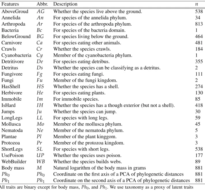
Table 3.1 Summary of the two methods used to predict interactions : the KNN algorithm and random forests. . . 30 Table 3.2 The 26 binary traits and the three continuous traits used for the

super-vised learning algorithm. . . 32 Table 3.3 Fictional example to illustrate recommendations withK nearest

neigh-bour using the Tanimoto distance measure modified to include species traits. . . 34 Table 3.4 Top1 success rates for theKNN/Tanimoto algorithm with various K and

weights to traits. . . 39

Table 4.1 Full confusion matrix forKNN algorithm with K=3 and threshold of 0.0 and 0.5 (majority vote). . . 53

Table 5.1 The input variables along with their abbreviation and range. All ranges are in millimetres except generalism and theKNN ratio. . . 63 Table 5.2 Definitions of conjunction (“and”, ∧) and disjunction (“or”, ∨)

follo-wing different norms. . . 67 Table 5.3 Full confusion matrix before and after theory revision with our fuzzy

algorithm using the product norm. . . 70 Table 5.4 TSS scores for our fuzzy logic approach along with standard supervised

learning algorithms. . . 70 Table 5.5 Example of a knowledge base after the theory revision algorithm

(17)

Table 5.6 Rules with the highest improvements in TSS when added to the initial knowledge base. . . 72

Table 6.1 Different languages can be distinguished by their ontological and epis-temological commitments. . . 80 Table 6.2 List of common binary connectives and their truth table with T standing

for True and F for False. . . 81 Table 6.3 The 18 predicates of the Salix data-set with their two domains : species

and location. . . 96 Table 6.4 How evaluation works in type-2 interval fuzzy logic. . . 102

(18)

LISTE DES FIGURES

Figure 1.1 Le metaweb et la représentation des interactions . . . 4 Figure 1.2 Apprentissage supervisé . . . 7 Figure 1.3 Apprentissage non supervisé . . . 7

Figure 2.1 McCarthy’s “Program with Common Sense” established the impor-tance of separating knowledge from reasoning. . . 13 Figure 2.2 Reasoning in Bayesian networks. . . 15 Figure 2.3 Various reasoning languages and their ability to model uncertainty,

vagueness, and relations . . . 20

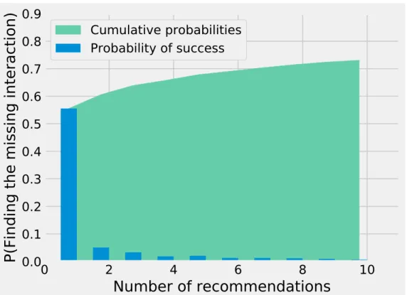
Figure 3.1 Finding the missing interaction withKNN/Tanimoto approach. . . 37 Figure 3.2 Success on first guess with Tanimoto similarity as a function of the

number of prey. . . 38

Figure 4.1 TSS scores for the KNN algorithm with K ranging from from 1 to 11 (odd integers only) and thresholds from 0 to 0.9. . . 52 Figure 4.2 Accuracy for theKNN algorithm with various values K and threshold,

defined as the number of correct predictions divided by the total num-ber of predictions. . . 53 Figure 4.3 Heatmap for the true positive rate (also called recall or sensitivity) of

(19)

Figure 4.4 Heatmap for the true negative rate (also called recall or sensitivity) of

theKNN with threshold. . . 55

Figure 5.1 Example of fuzzy sets. . . 65

Figure 5.2 Mean TSS on the testing data for the three T−norm tested studied and 3, 5, 7, 9, or 11 fuzzy sets per input variables. . . 71

Figure 6.1 Inference in Bayesian networks. . . 88

Figure 6.2 An example of Markov logic networks. . . 89

Figure 6.3 Inference in Markov logic networks. . . 94

Figure 7.1 Prédicats flous et logique de Markov . . . 110

(20)

CHAPITRE 1

INTRODUCTION GÉNÉRALE

1.1 La grande obsession

Au début du vingtième siècle, Sewall Wright, Ronald Fisher, et J.B.S. Haldane développent une théorie de l’évolution, la synthèse moderne, basée principalement sur la sélection naturelle, la dérive génétique, et les mutations (Provine, 2001). Suite au progrès en génétique moléculaire, il devient enfin possible dans les années 60 de mesurer la diversité génétique de façon précise (Lewontin et Hubby, 1966). Les résultats sont problématiques pour les théoriciens : il y a beaucoup plus de diversités qu’on s’y attendait (Provine, 2001). La réponse, la théorie neutre, veut que la sélection soit un phénomène marginal (Kimura, 1968 ; King et Jukes, 1969 ; Kimura, 1983). Cette théorie a le mérite d’être simple à paramétriser mais des découvertes modernes en génomique des populations montrent que la sélection est commune (Gillespie, 2004 ; Begun et al., 2007). Malheureusement, nous avons peu d’alternatives théoriques viables au modèle neutre (Hahn, 2008).

Pourquoi la biodiversité est-elle si complexe d’un point de vue théorique ? Il y a plusieurs raisons, tant au niveau du génome qu’au niveau des populations. L’effet d’une mutation varie énormément d’un endroit à l’autre. Sur le même gène, une mutation peut grandement influencer la fonction du gène alors qu’une mutation à proximité aura peu d’influence. Cette complexité complique l’analyse des mutations, qui est souvent réduite à comparer les mutations où le nu-cléotide d’un codon est changé à celle qui ne change pas le nunu-cléotide (mutations silencieuses) (Hahn, 2008). Cette simplification ignore la majorité des facteurs qui influencent l’effet d’une mutation sur le phénotype (Wilke, 2012).

Au niveau des populations, la sélection varie dans l’espace et le temps alors que l’environne-ment biotique et abiotique change. Loin d’être une force constante qui pousse certaines muta-tions vers la fixation ou l’extinction, la sélection change constamment en fonction de l’environ-nement. Une population a des proies, des compétiteurs, des prédateurs différents d’un endroit

(21)

à l’autre, ce qui a pour effet de créer des pressions sélectives différentes dans chaque commu-nauté. Ces pressions changent aussi avec le temps alors que la composition de la communauté se transforme (Bell, 2010).

Aux deux facteurs précédents doit s’ajouter le déséquilibre de liaison (Lynch, 2007), qui est de plus en plus considéré comme un facteur important pour comprendre la diversité du génome (Begun et al., 2007). Une mutation positive qui se trouve localisée près d’une mutation désa-vantageuse va favoriser la progression de cette dernière dans la population. Bref, non seulement la pression sélective sur les traits (et donc les gènes) varie dans le temps et l’espace, mais cette pression a des conséquences sur les loci rapprochés sur le chromosome. L’intégration du dés-équilibre de la liaison dans une théorie de la biodiversité moléculaire est une priorité pour les théoriciens mais elle demeure difficile sans l’ajout de plusieurs paramètres (Hahn, 2008). Dernièrement, la spéciation a une structure spatiale complexe (Gravilets, 2004). La majorité des évènements de spéciation surviennent lorsqu’une population est partiellement ou complè-tement isolée du reste de l’espèce. C’est la spéciation allopatrique. Rarement, des populations au même endroit deviennent isolées au niveau de la reproduction (spéciation sympatrique) (Coyne et Orr, 2004). J’ai consacré mes premiers articles à développer une version de la théo-rie neutre de la biodiversité qui intègre la notion d’isolation géographique (Annexes A, B, C). Ultimement, les nouvelles espèces peuvent occuper des niches différentes. La spéciation a donc un rôle important pour comprendre la biodiversité au niveau des communautés.

En bref, la biodiversité est difficile sur le plan théorique parce qu’elle implique beaucoup de facteurs et que nous avons rarement assez d’informations pour paramétriser des modèles plus sophistiqués que des théories neutres. Il est donc difficile de capturer l’essence de la biodiver-sité avec des modèles théoriques suffisamment simples. Hahn (2008) note : the consequence of this is that we have tied ourselves into philosophical knots by using null models no one believes but are easily parameterized. Si l’ambition des théoriciens de découvrir une grande théorie de la biodiversité est vaine, il faut explorer des alternatives. Une avenue possible se-rait d’utiliser des techniques en intelligence artificielle pour combiner, à l’intérieur d’une base de connaissance unifiée, plusieurs théories. Au lieu de chercher une théorie de la biodiver-sité, notre rôle serait alors de trouver comment combiner plusieurs théories. Pour cette thèse, je vais explorer diverses représentations de la connaissance et leur potentiel pour la synthèse d’idées en écologie, et comment exploiter ces représentations par des techniques d’apprentis-sages automatiques. J’utiliserai des données sur les interactions entre les espèces pour tester

(22)

ces techniques.

1.2 Interaction des espèces

Toutes les données utilisées pour cette thèse se rapportent à l’interaction des espèces (Pimm, 1982) (Figure 1.1). Ce problème a été choisi pour deux raisons. Primo, l’interaction des espèces est une des raisons expliquant pourquoi la biodiversité est si difficile à modéliser (Bartomeus et al., 2016). Une théorie générale de la biodiversité devrait inclure de solides prédictions sur les interactions pour comprendre quelles forces influencent les populations. Secondo, plusieurs membres du laboratoire étudient les interactions, ce qui me donne accès à la fois à des données de qualité mais aussi à des gens capables de les interpréter.

Les données utilisées pour cette thèse proviennent de trois ensembles de données :

— Le premier, assemblé par Idaline Laigle, contient plus de 30 000 interactions obser-vées parmi près de 900 espèces. Pour chaque espèce, nous avons les informations sur 28 traits (la taille, si l’espèce est sous la terre, sa taxonomie, etc.). Ces données sont détaillées à la sous-section 3.4.1 et à la table 3.2.

— Le second, utilisé dans les chapitres 4 et 5, couvre les interactions entre pollinisateurs et plantes. Il contient plus de 700 observations ainsi que plusieurs traits pour les polli-nisateurs et les plantes. Il est décrit en détail aux sous-sections 4.3.1 et 5.4.1 ainsi qu’à la table 5.1.

— Le dernier a été assemblé par notre laboratoire et ses collaborateurs, il contient un réseau d’interactions tritrophiques avec des interactions entre parasites et insectes, et des interactions entre ces insectes et des saules. Il a été collecté sur plusieurs sites en Europe et contient des informations sur les précipitations et la température moyenne sur chacun de ces sites. Il est décrit à la section 6.7, la table 6.3, ainsi que dans l’article de Kopelke et al. (2017).

Le problème est intéressant d’un point de vue théorique dans le sens où il peut être approché de plusieurs façons. On peut vouloir prédire une interaction à partir des traits des espèces, en se basant sur les interactions d’une espèce similaire. On peut considérer les pairs d’espèces qui n’ont pas d’interactions comme une absence d’évidence (approche par recommandation) ou

(23)

Figure 1.1 – Le metaweb et la représentation des interactions

Le metaweb (à droite) et des réseaux d’interactions locaux (à gauche). Les espèces sont représentées par des formes de couleurs différentes. Deux espèces peuvent interagir dans une communauté locale et non dans une autre, comme par exemple le cercle blanc et le carré blanc, qui ont une interaction dans la communauté 3 mais pas dans la 1. Le metaweb est la collection de toutes les interactions locales. Il est souvent présumé que si une espèce interagit avec une autre dans une communauté, elle le fera aussi dans toutes les autres communautés, mais ce n’est pas le cas. La figure provient de Poisot et al. (2012).

une évidence d’absence (complétion de matrice). Ces données ont cependant des limites. Les interactions sont bivalentes, soit deux espèces ont une interaction, soit elles n’en n’ont pas. Les données ignorent aussi les interactions qui pourraient impliquer plus d’une espèce.

1.3 Deux questions

Ma thèse s’attaque à deux questions : quelle représentation des connaissances permet de repré-senter les théories en écologie ? Comment réviser automatiquement des théories écologiques formulées avec cette représentation ?

(24)

Ces deux questions mènent à deux branches de l’intelligence artificielle : la représentation des connaissances et l’apprentissage automatique (machine learning).

Pour être clair, la question ici n’est pas de savoir comment représenter les données écologiques, mais bien de représenter les théories. Par exemple, on voudrait pouvoir représenter des théories comme l’équation de Lotka-Volterra, le modèle de niche (Williams et Martinez, 2000) ou des théories probabilistiques comme la théorie neutre de Hubbell (2001).

1.4 Représentation des connaissances

Les théories en écologie se distinguent des modèles mathématiques par leur flexibilité : per-sonne ne s’attend à ce qu’un modèle qui prédit la population d’une espèce soit exact, alors que les modèles en physique et les bases de théorèmes mathématiques s’accomodent facilement de la bivalence (tout est soit vrai, soit faux, sans nuance). Le chapitre 2 explique en détails en quoi la représentation des théories écologiques est un sujet difficile (Russell et Norvig, 2009).

1.5 Apprentissage automatique

Le second ingrédient est l’apprenttisage automatique : la capacité de bâtir des modèles (ou de réviser des modèles existants) automatiquement à partir de données. Il existe deux grandes branches : l’apprentissage supervisé (Figure 1.2) et l’apprentissage non supervisé (Figure 1.3). Ces deux approches seront utilisées lors de la thèse. Selon l’approche supervisée, les données

D sont formées d’un vecteur de featuresx et d’une sortie y (ce qu’on veut prédire) :

D = {(x_i, yi)}

|D|−1

i=0 . (1.1)

Siy est un nombre entier, on a un problème de classification et si c’est un nombre réel, on a un problème de régression. La régression n’est pas explorée lors de cette thèse, mais les chapitres 3 et 5 traitent du problème d’interaction des espèces comme un problème de classification. x représente les traits de deux espèces et y dénote si ces espèces interagissent. Le chapitre

(25)

3 utilise plusieurs méthodes standards en apprentissage supervisé comme les decision trees, les support vector machines et les random forests (Murphy, 2012). Le chapitre 5 utilise une méthode que j’ai développé pour apprendre des règles simples en logique floue pour prédire si un pollinisateur et une plante interagissent.

L’approche non supervisée est plus difficile à décrire formellement. Elle implique de trouver des structures intéressantes à l’intérieur des données :

D = {(xi)} |D|−1

i=0 . (1.2)

Plusieurs méthodes non supervisées sont utilisées. On peut voir le problème des interactions comme un problème de complétion de matrice (chapitres 3 et 4) : la matrice représente les interactions, les trous dans la matrice représentent des paires d’espèces, et l’objectif est de remplir ces trous soit par une interaction ou une non-interaction. On peut aussi voir le pro-blème comme un système de recommandations (chapitre 3), ou chaque espèce a un groupe de proies et on tente de suggérer à cette espèce des proies éventuelles, à la manière dont Netflix ou Amazon tente de prédire les items qui peuvent vous intéresser en se basant sur des uti-lisateurs qui vous ressemblent ou des items qui ressemblent à celui qui vous intéresse. Cette approche a l’avantage de considérer seulement les évidences positives et d’ignorer les absences d’interactions. Étant donné qu’il est difficile en pratique de confirmer que deux espèces n’ont pas d’interactions, cette méthode est particulièrement appropriée pour étudier les interactions. Finalement, le chapitre 6 explore l’apprentissage de règles relationelles, une autre branche de l’apprentissage non supervisé (Richardson et Domingos, 2006). Les approches relationelles sont expliquées brièvement au chapitre 2, et plus en détails au chapitre 6.

(26)

Figure 1.2 – Apprentissage supervisé

L’approche supervisée consiste à prédire un labely à partir des features x. Figure de Murphy (2012).

Figure 1.3 – Apprentissage non supervisé

L’approche non supervisée est plus difficile à définir, elle consiste à découvrir des structures intéres-santes dans les données. Ici, on voit l’exemple de complétion de matrice, ici une image avec un trou. L’objectif est de trouver de bonnes valeurs pour remplir ce trou. Figure de Murphy (2012).

(27)

1.6 Le plan de la thèse

La thèse se sépare en sept chapitres : l’introduction, cinq articles, et une conclusion générale. Le chapitre 2 explore la relation entre l’intelligence artificielle et les théories scientifiques, en mettant l’emphase sur les théories en écologie et le besoin d’étudier des représentations plus flexibles que celles adoptées par les mathématiciens. Les chapitres 3 et 4 appliquent des algo-rithmes standards en intelligence artificielle au problème d’interactions des espèces. Bien que ces deux chapitres ne touchent pas directement à la question de révision des théories scienti-fiques, les leçons apprises lors de ces recherches m’ont servi lors de mes travaux sur la révision automatique. Le chapitre 5 étudie une nouvelle approche pour apprendre des règles avec la lo-gique floue. Appliquée à des interactions pollinisateurs-plantes, cette technique nous permet de réviser une théorie de base simple pour arriver à un modèle à la fois plus clair et plus efficace que les techniques standards en intelligence artificielle. Le chapitre 6 explore la logique de Markov. Cette technique n’a pas bien fonctionnée, mais elle donne d’importantes pistes pour l’étude d’approches capables d’intégrer des théories mathématiques et la révision automatique. Ce chapitre termine avec une discussion sur les prochaines étapes pour progresser sur la ques-tion de révision automatique de théories écologiques. La conclusion générale boucle la thèse en retournant sur les deux questions posées dans cette introduction.

(28)

CHAPITRE 2

ECOLOGICAL SYNTHESIS AND ARTIFICIAL INTELLIGENCE

2.1 Description de l’article et contribution

Avant de pouvoir réviser des théories écologiques avec des techniques d’intelligence artifi-cielle, il faut choisir une représentation de la connaissance pour les théories écologiques. Dans cette contribution, nous explorons diverses représentations de la connaissance et comment celles-ci peuvent servir à encoder les théories écologiques. Les mathématiciens ont depuis plu-sieurs décennies assemblé de larges bases de connaissances en utilisant une forme de logique (predicate logic). Malheureusement, cette forme de logique est trop inflexible pour l’écologie. On ne s’attend pas, contrairement aux mathématiciens et aux physiciens, à ce que nos théo-ries soient toujours exactes. La complexité des écosystèmes nous force à accepter des théothéo-ries imparfaites, mais utiles. Combiner ces théories dans un tout est d’autant plus complexe que relativement peu de travail a été fait pour assembler les théories inexactes. Cet article discute de différents systèmes de raisonnement allant des probabilités à la logique pure, ainsi que la logique floue. Nous expliquons pourquoi l’intégration de théories écologiques et la révision de celles-ci requièrent que l’on réfléchisse à la structure des connaissances écologiques.

J’ai conçu et fait la recherche de cet article de perspective. Dominique Gravel et Timothée Poisot m’ont assisté pour la révision. L’article a été publié sur bioRxiv. Cet article servira de base pour une revue de littérature sur l’union de l’intelligence artificielle et des théories écologiques qui sera soumis à un numéro spécial de Frontiers in Ecology and Evolution.

(29)

2.2 Ecological Synthesis

Artificial Intelligence presents an important paradigm shift for science. Science is traditionally founded on theories and models, most often formalized with mathematical formulas handcraf-ted by theoretical scientists and refined through experiments. Machine learning, an important branch of modern Artificial Intelligence, focuses on learning from data. This leads to a fun-damentally different approach to model-building : we step back and focus on the design of algorithms capable of building models from data, but the models themselves are not desi-gned by humans. This is even more true with deep learning, which requires little engineering by hand and is responsible for many of Artificial Intelligence’s spectacular successes (LeCun et al., 2015). In contrast to logic systems, knowledge from a deep learning model is difficult to understand, reuse, and may involve up to a billion parameters (Coates et al., 2013). On the other hand, probabilistic machine learning techniques such as deep learning offer an opportu-nity to tackle large complex problems that are out of the reach of traditional theory-making. It is possible that the more intuition-like (LeCun et al., 2015) reasoning performed by deep learning systems is mostly incompatible with the logic formalism of mathematics. Yet recent studies have shown that deep learning can be useful to logic systems and vice versa. Success at unifying different paradigms of Artificial Intelligence from logic to probability theory offers unique opportunities to combine data-driven approaches with traditional theories. These ad-vancements are susceptible to impact significantly theoretical work on ecology and evolution, allowing for the integration of data and theories in unified knowledge bases.

Ever since molecular biology allowed for precise measurements of molecular diversity, theo-reticians have struggled to explain why populations are so diverse (Lewontin et Hubby, 1966 ; Gillespie, 2004 ; Hahn, 2008). Integrating selection proved hard enough for neutral theories to dominate in practice since few solid alternatives are easy enough to parameterize (Hahn, 2008). Theoretical ecology has had a similar struggle with similar consequences, Hubbell’s neutral theory of biodiversity is almost exactly the same as Kimura’s neutral theory of mole-cular evolution, with alleles being different species and point mutation being replaced by point speciation (Kimura, 1983 ; Hubbell, 2001).

Recent work in population genomics show the importance of linkage Begun et al. (2007) and point to a world where selection is a constant presence in the genome, not as a simple force pushing mutations toward extinction or fixation, but as a stochastic mechanism varying in time

(30)

and space Bell (2010). In Toward a Selection Theory of Molecular Evolution, Matthew Hahn noted how population geneticists became dependant on neutral theories and have effectively “tied [themselves] into philosophical knots by using null models no one believes but are easily parameterized” Hahn (2008). Thus, interestingly, the reason a truly unified theory of biodiver-sity has proven elusive is not because we do not know the basic mechanisms involved, it is because we do not how to effectively build a theory simple enough to be usable.

Our thesis is that biodiversity is unlikely to simplify to a single elegant equation. In that case, we could turn to and tools from A.I. to help us integrate various ecological and evolutionary ideas into a single unified knowledge base. Instead of looking for a single theory, we would grow knowledge, similarly to how mathematicians have build large knowledge bases of theo-rems (Kaliszyk et Urban, 2015). However, ecology and evolution are not pure mathematics, we do not expect our ideas to be as precise as theorems. Thus, the question becomes : what is the correct knowledge representation for ideas in ecology and evolution ?

2.3 A.I. and knowledge representation

Science would greatly benefit from a unification of Artificial Intelligence with traditional ma-thematical theories. Modern research at the intersection of logic, probability theory, and fuz-ziness yielded rich representations increasingly capable of formalizing scientific knowledge. Such formal corpus could both include hand-crafted theories from Einstein’se = mc2 to the Breeder’s equation (Rice, 2004), but also harness modern A.I. algorithms for testing and lear-ning. Comprehensive synthesis is difficult in fields like biology, which have not been reduced to a small set of formulas. For example, while we have a good idea of the underlying forces dri-ving evolution, we struggle to build effective predictive models of molecular evolution (Hahn, 2008). This is likely because selection changes in time and space (Bell, 2010), which brings population, community, and ecosystem ecology into the mix. Ecology also has a porous fron-tier with evolution : speciation is a common theme in community ecology theory (Desjardins-Proulx et Gravel, 2012).

From a theoretical perspective, work to formalize scientific theories would reveal much about the nature of our theories. Surely, scientific theories require more flexibility than mathematical corpora of knowledge, which are based on pure logic. From a practical standpoint, a formal

(31)

representation both offers ways to test large corpora of knowledge and extend it with A.I. tech-niques. This is arguably the killer feature of a formal representation of scientific knowledge : allowing A.I. algorithms to search for revisions, extensions, and discover new rules. This is not a new ambition. Generic techniques for rule discovery were well-established in the 1990s (Muggleton et de Raedt, 1994). Unfortunately, these techniques were based on pure logic, and purely probabilistic approaches to revision cannot handle mathematical theories. Recent expe-riences in linguistics has shown that building a knowledge base capable of handling several problems at the same time yielded better results than attacking the problem in isolation be-cause of the problems’ interconnectedness (Yoshikawa et al., 2009). Biology, as a complex field made of more-or-less arbitrary subfields, could gain important insights from unified ap-proach to knowledge combining A.I. techniques with traditional mathematical theories.

2.4 A quick tour of knowledge representations

Deep learning is arguably the dominant approach in probabilistic machine learning, a branch of A.I. focused on learning models from data (Goodfellow et al., 2016). The idea of deep learning is to learn multiple levels of compositions. If we want to learn to classify images for instance, the first layer of the deep learning network will read the input, the next layer will capture lines, the next layer will capture contours based on lines, and then more complex shapes based on contours, and so on (Goodfellow et al., 2016). In short, the layers of the network begin with simple concepts, and then compose more complicated concepts from simpler ones (Bengio et al., 2013). Deep learning has been used to solve complex computer science problems like playing Go at the expert level (Silver et al., 2016), but it is also used for more traditional scientific problems like finding good candidate molecules for drugs, predicting how changes in the genotype affect the phenotype (Leung et al., 2016), or just recently to solving the quantum many-body problem (Carleo et Troyer, 2017).

In contrast, traditional scientific theories and models are mathematical, or logic-based. Ein-stein’se =mc2established a logical relationship between energye, mass m, and the speed of light c. This mathematical knowledge can be reused : in any equation with energy, we could replacee with mc2. This ability of mathematical theories to establish precise relationships bet-ween concepts, which can then be used as foundations for other theories, is fundamental to how science grows and forms an interconnected corpus of knowledge. Furthermore, these theories

(32)

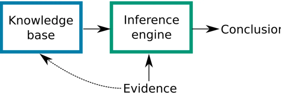
Figure 2.1 – McCarthy’s “Program with Common Sense” established the importance of separa-ting knowledge from reasoning.

Knowledge

base

Inference

engine

Conclusion

Evidence

In his 1959’s “Programs with Common Sense”, McCarthy established the importance of separating knowledge and reasoning (McCarthy, 1959). The knowledge base stores knowledge, while the infe-rence engine exploits it, along with evidence, to reach conclusions. McCarthy believed the knowledge base should store rules in some form of predicate logic, but the idea of separation of knowledge and reasoning holds with other representations as well (Bayesian networks, detailed in figure 2.2, are proba-bilistic knowledge bases (Darwiche, 2009)). The dotted line represents automatic theory revision, where evidence is used not to a answer query but to discover new knowledge or revise existing theories.

are compact and follow science’s tradition of preferring theories as simple as possible. There are many different foundations for logic systems. Predicate logic is a good starting point : it is based on predicates, which are functions of terms to a truth value. For example, the predicate PreyOn could take two species, a location, and return true if the first species preys on the se-cond at that location, likePreyOn(Wolverine, Squirrel, Quebec). Terms are either constants such as 1, π, or Wolverine, variables that range over constants, such as x or species, or func-tionsthat map terms to terms, such as additions, multiplication, integration, differentiation. In e = mc2, the equal sign =is the predicate,e and m are variables, c and 2 are constants, and there are two functions : the multiplication ofm by c2and the the exponentiation ofc by 2. The key point is that such formalism lets us describe compact theories and understand precisely how different concepts are related. Complex logic formulas are built by combining predicates with connectives such as negation¬, “and”∧, “or”∨, “implication”⇒. We could have a rule to say that predation is asymmetricalsx ̸= sy∧PreyOn(sx, sy, l) ⇒ ¬PreyOn(sy, sx, l), or define the classical Lotka-Volterra :

dx

dt =αx−βxy∧ dy

(33)

wherex and y are the population sizes of the prey and the predator, respectively, α, β, δ, γ are constants, and the time differentiald/dt, multiplication and subtraction are functions. Equality (=) is the sole predicate in this formula. Both predicates are connected via ∧ (“and”). Not all logic formulas have mathematical functions. Simple logic rules such as Smoking(p) ⇒

Cancer(p)(“smoking causes cancer”) are common in expert systems.

Artificial Intelligence researchers have long being interested in logic systems capable of scien-tific discoveries, or simply capable of storing scienscien-tific and medical knowledge in a single coherent system (Figure 2.1). DENDRAL, arguably the first expert system, could form hypo-theses to help identify new molecules using its knowledge of chemistry (Lindsay et al., 1993). In the 1980s, MYCIN was used to diagnose blood infections (and did so more accurately than professionals) (Buchanan et Shortliffe, 1984). Both systems were based on logic, with MYCIN adding a “confidence factor” to its rules to model uncertainty. Other expert systems were based on probabilistic graphical models (Koller et Friedman, 2009), a field that unites graph theory with probability theory to model the conditional dependence structure of random variables (Koller et Friedman, 2009 ; Barber, 2012). For example, Munin had a network of more than 1000 nodes to analyze electromyographic data (et al., 1996), while PathFinder assisted medi-cal professional for the diagnostic of lymph-node pathologies (Heckerman et Nathwani, 1992) (Figure 2.2). While these systems performed well, they are both too simple to store generic scientific knowledge and too static to truly unify Artificial Intelligence with scientific research. The ultimate goal is to have a representation rich enough to encode both logic-mathematical and probabilistic scientific knowledge.

(34)

Med Lymph Cells

LLC Num

MLC Num

LLC+MLC > 50% P(L) = 0.81

A Bayesian network with four binary variables and possible conditional probability tables. These four nodes were taken from PathFinder, a Bayesian network with more than 1000 nodes used to help diag-nose blood infections (Heckerman et Nathwani, 1992). The nodes represent four variables related to blood cells and are denoted by a single character (in bold in the figure) : C, M, L,+. All variables are binary, and negation is denoted with ¬. Since P(¬x|y) = 1−P(x|y), we need only 2|Pa(x)| parameters per nodes, with |Pa(x)| being the number of parents of node x. The structure of Baye-sian networks both highlights the conditional independence assumptions of the distribution and re-duces the number of parameters for learning and inference. Example query : P(L,¬C, M,¬+) =

P(L)P(¬C)P(M|¬C)P(¬ + |L,¬C, M) = 0.81× (1−0.65) ×0.27× (1−0.42) = 0.044. See (Darwiche, 2009) for a detailed treatment of Bayesian networks and (Koller et Friedman, 2009) for a more general reference on probabilistic graphical models.

(35)

2.5 Beyond monolithic systems

In terms of representation, expert systems generally used a simple logic system, not power-ful enough to handle uncertainty, or purely probabilistic approaches unable to handle complex mathematical formulas. In terms of flexibility, the expert systems were hand-crafted by human experts. After the experts established either the logic formulas (for logic systems like DEN-DRAL) or probabilistic links (in the case of systems like Munin), the expert systems act as static knowledge bases, capable of answering queries but unable of discovering new rules and relationships. While no system has completely solved these problems yet, much energy has been put in unifying logic-based systems with probabilistic approaches (Getoor et al., 2007). Also, several algorithms have been developed to learn new logic rules (Muggleton et de Raedt, 1994), find the probabilistic structure in a domain with several variables (Yuan et Malone, 2013), and even transfer knowledge between tasks (Mihalkova et al., 2007). Together, these discoveries bring us closer to the possibility of flexible knowledge bases contributed both by human experts and Artificial Intelligence algorithms. This has been made possible in great part by efforts to unify three distinct languages : probability theory, predicate logic, and fuzzy logic (Figure 2.3).

The core idea behind unified logic/probabilistic languages is that formulas can be weighted, with higher values meaning we have greater certainty in the formula. In pure logic, it is im-possible to violate a single formula. With weighted formulas, an assignment of concrete values to variables is only less likely if it violates formulas. The higher the weight of the formula violated, the less likely the assignment is. It is conjectured that all perfect numbers are even (∀x : Per f ect(x) ⇒ Even(x)), if we were to find a single odd perfect number, that formula would be refuted. It makes sense for mathematics but for many disciplines, such as biology, important principles are only expected to be true most of the times. To illustrate, in ecology, predators generally have a larger body weight than their preys, which can expressed in predicate logic as PreyOn(predator, prey) ⇒ M(predator) > M(prey), with M(x) being the body mass of x. This is obviously false for some assignments, for example predator : greywol f and prey : moose. However, it is useful knowledge that underpins many ecological theories (Williams et Martinez, 2000). When our domain involves a great number of variables, we should expect useful rules and formulas that are not always true.

(36)

logic formulas to be weighted (Richardson et Domingos, 2006 ; Domingos et Lowd, 2009). It supports algorithms to add weights to existing formulas given a data-set, learn new formulas or revise existing ones, and answer probabilistic queries. For example, Yoshikawa et al. used Markov logic to understand how events in a document were time-related (Yoshikawa et al., 2009). Their research is a good case study of interaction between traditional theory-making and artificial intelligence. The formulas they used as a starting point were well-established logic rules to understand temporal expressions. From there, they used Markov logic to weight the rules, adding enough flexibility to their system to beat the best approach of the time. Brouard et al. (Brouard et al., 2013) used Markov logic to understand gene regulatory network, noting how the resulting model provided clear insights, in contrast to more traditional machine learning techniques. Expert systems can afford to make important sacrifices to flexibility in exchange for a simple representation. Yet, a system capable of representing a large body of scientific knowledge will require a great deal of flexibility to accommodate various theories. While a step in the right direction, even Markov logic may not be powerful enough.

2.6 Case study : The niche model

To show some of the difficulties of representing scientific knowledge, we will build a small knowledge base for an established ecological theory : the niche model of trophic interactions (Williams et Martinez, 2000). The first iteration of the niche model posits that all species are described by a niche position N (their body size for instance) in the[0, 1] interval, a dietD in the [0, N] interval, and a range R such that a species preys on all species with a niche in the

[D−R/2, D+R/2]interval. We can represent these ideas with three formulas :

∀x, y :¬PreyOn(x, y), (2.2a)

∀x : D(x) < N(x), (2.2b)

(37)

where ∀ reads for all and ⇔ is logical equivalence (it is true if and only if both sides of the operator have the same truth value, so for exampleFalse⇔False is true and True ⇔False is false). As pure logic, this knowledge base makes little sense. Formula 2.2a is obviously not true all the time. It is mostly true, since most pairs of species do not interact. We could also add that cannibalism is rare ∀x : ¬PreyOn(x, x) and that predator-prey are generally asymmetrical

∀x, y : PreyOn(x, y) ⇒ ¬PreyOn(y, x). In hybrid probabilistic/logic approaches like Mar-kov logic, these formulas would have a weight that essentially defines a marginal probability (Domingos et Lowd, 2009 ; Jain, 2011). Formulas that are often wrong are assigned a lower weight but can still provide useful information about the system. The second formula says that the diet is smaller than the niche value. The last formula is the niche model : species x preys ony if and only if species y’s niche is within the diet interval of x.

So far so good ! Using Markov logic networks and a data-set, we could learn a weight for each formula in the knowledge base. This step alone is useful and provide insights into which formulas hold best. With the resulting weighted knowledge base, we could make probabilis-tic queries and even attempt to revise the theory automaprobabilis-tically. We could find, for example, that the second rule does not apply to parasites or some group and get a revised rule such as

∀x : ¬Parasite(x) ⇒ D(x) < N(x). However, Markov logic networks struggle when the predicates cannot easily return a simple true-or-false truth values. For example, let’s say we wanted to express the idea that when populations are small and have plenty of resources, they grow exponentially (Kot, 2001).

∀x, l, t : SmallP(x, l, t)andResources(x, l, t) ⇒ P(x, l, t+1) = G(x) ×P(x, l, t), (2.3)

where P(x, l, t) is the population size of species x in location l at time t, G is the rate of growth, SmallP is whether the species has a small population and Resources whether it has resources available. The problem with hybrid probabilistic/logic approach is that predicates do not capture the inherent vagueness well. We can establish an arbitrary cutoff for what a small population is, for example by saying that if it is less than 10% the average population size for the species, it is small. Similarly, resource availability is not a binary thing, there is a world of grey between starvation and satiety. Perhaps worst of all, the prediction that P(x, l, t+1) = G(x) ×P(x, l, t) is almost certainly never be exactly true. If we predict 94

(38)

rabbits and observe 93, the formula is false. Weighted formulas help us understand how often a rule is true, but in the end the formula has to give a binary truth value : true or false, there is no place for vagueness.

Fuzzy sets and many-valued (“fuzzy”) logics were invented to handle vagueness (Zadeh, 1965 ; Hájek, 1998 ; Bergmann, 2008 ; Behounek et al., 2011). In practice, it simply means that pre-dicates can return any value in the[0, 1]closed interval instead of only true and false. It is used in both probabilistic soft logic (Kimmig et al., 2012 ; Bach et al., 2015) and deep learning ap-proaches to predicate logic (Zahavy et al., 2016 ; Hu et al., 2016). For our formula 2.3,SmallP could be defined as1−P(x, l, t)/Pmax(x), wherePmax(x)is the largest observed population size for the species. Resources could take into account how many preys are available, and P(x, l, t+1) = G(x) ×P(x, l, t)would return a truth value based on how close the observed population size is the predicted population size. Fuzzy logic then defines how operators such asand and⇒behave with fuzzy values.

Both Markov logic networks and probabilistic soft logic define a probability distribution over logic formulas, but what about the large number of probabilistic models ? For example, the niche model has a probabilistic counter-part defined as (Williams et al., 2010) :

∀x, y : PPreyOn(x, y) = α×exp [ −( N(y) −D(x) R(x)/2 )2] , (2.4)

wherePPreyOn(x, y) is the probability thatx preys on y. Again, this formula is problematic in Markov logic because we cannot easily force the equality into a binary true-or-false, but fuzziness can help model the nuance of probabilistic predictions. There are no algorithms yet to learn and revise rules in many-valued logic.

(39)

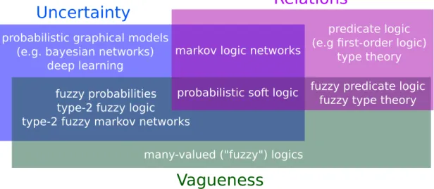
Figure 2.3 – Various reasoning languages and their ability to model uncertainty, vagueness, and relations.

Uncertainty

probabilistic graphical models (e.g. bayesian networks)

deep learning

Relations

Vagueness

many-valued ("fuzzy") logics fuzzy probabilities

type-2 fuzzy logic type-2 fuzzy markov networks

markov logic networks

predicate logic (e.g ﬁrst-order logic)

type theory probabilistic soft logic fuzzy predicate logic

fuzzy type theory

The size of the rectangles has no meaning. In the blue rectangle : languages capable of handling uncer-tainty. Probabilistic graphical models combine probability theory with graph theory to represent com-plex distributions (Koller et Friedman, 2009). Deep learning is, strictly speaking, more general than its usual probabilistic interpretation, but it is arguably the most popular probabilistic Artificial Intelligence approach at the moment (Goodfellow et al., 2016). Alternatives to probability theory for reasoning about uncertainty include possibility theory and Dempster-Shafer belief functions, see (Halpern, 2003) for an extended discussion. In the green rectangle : Fuzzy logic extends standard logic by allowing truth values to be anywhere in the[0, 1]interval. Fuzziness models vagueness and is particularly popular in linguistics, engineering, and bioinformatics, where complex concepts and measures tend to be vague by nature. See (Kosko, 1990) for a detailed comparison of probability and fuzziness. In the purple rec-tangle : relations, as in : mathematical relations between objects. Even simple mathematical ideas, such as the notion that all natural numbers have a successor (∀x∃y : y= x+1), requires relations. Predicate and Relation are synonymous in this context. Alone, these reasoning languages are not powerful enough to express scientific ideas. We must thus focus on what lies at their intersection. Type-2 Fuzzy Logic is a fast-expanding (Sadeghian et al., 2014) extension to fuzzy logic, which, in a nutshell, models uncer-tainty by considering the truth value itself to be fuzzy (Mendel et Bob John, 2002 ; Zeng et Liu, 2008). Markov logic networks (Richardson et Domingos, 2006 ; Domingos et Lowd, 2009) extends predicate logic with weights to unify probability theory with logic. Probabilistic soft logic (Kimmig et al., 2012 ; Bach et al., 2015) also has formulas with weights, but allow the predicates to be fuzzy, i.e. have truth values in the[0, 1]interval. Some recent deep learning studies also combine all three aspects (Garnelo et al., 2016 ; Hu et al., 2016).

(40)

2.7 Where’s our unreasonably effective paradigm ?

Wigner’s Unreasonable Effectiveness of Mathematics in the Natural Sciences led to important discussions about the relationship between physics and its main representation (Wigner, 1960 ; Hamming, 1980). The Mizar Mathematical Library and the Coq library (The Coq development team, 2004) host tens of thousands of mathematical propositions to help build and test new proofs. In complex domains with many variables, Halevy et al. argued for the Unreasonable Effectiveness of Data (Halevy et al., 2009), noting that simple algorithms, when fed large amount of data, would do wonder. High-dimensional problems like image imputation, where an algorithm has to fill missing parts from an image, require hundred of thousands of training images to be effec-tive. Goodfellow et al. noted that roughly 10 000 data-points per possible labels were necessary to train deep neural networks (Goodfellow et al., 2016). These approaches are unsatisfactory for fields like biology where theories and principles are seldom exact. We cannot afford the pure logic-based knowledge representations favoured by mathematicians and physicists, and fitting a model to data is a different task than building a corpus of interconnected knowledge. Fortunately, we do not need to choose between mathematical theories, probabilistic models, and learning. New inventions such as Markov logic networks and probabilistic soft logic are moving Artificial Intelligence toward rich representations capable of formalizing and even ex-tending scientific theories. This is a great opportunity for synthesis. There are still problems : inference is often difficult in those rich representations. Recently, Garnelo et al. (Garnelo et al., 2016) designed a prototype to extract logic formulas from a deep learning system, while Hu et al. (Hu et al., 2016) created a framework to learn predicate logic rules using deep learning. Both studies used flexible fuzzy predicates and weighted formulas while exploiting deep lear-ning’ ability to model complex distributions via composition. The end result is a set of clear and concise weighted formulas supported by deep learning for scalable inference. The poten-tial for science is important. Not only these new researches allow for deep learning to interact with traditional theories, but it opens many exciting possibilities, like the creation of large da-tabases of scientific knowledge. The only thing stopping us from building a unified corpus of, say, ecological knowledge, is that normal pure-logic systems are too inflexible. They do not allow imperfect, partially-true theories, which are fundamental to many sciences. Recent de-velopments in Artificial Intelligence make these corpora of scientific knowledge possible for complex domains, allowing us to combine a traditional approach to theory with the power of Artificial Intelligence.

(41)

It is tempting to present deep learning as a threat to traditional theories. Yet, there is a real possibility that the union of Artificial Intelligence techniques with mathematical theories is not only possible, but would help the integration of knowledge across various disciplines. Other-wise, short of discovering a small set of elegant theories, what is our plan to combine ideas from ecosystem ecology, community ecology, population ecology, and evolution ?

2.8 References

Bach, S., Broecheler, M., Huang, B., Getoor, L. (2015). Hinge-loss markov random fields and probabilistic soft logic arXiv : 1505.04406.

Barber, D. (2012). Bayesian Reasoning and Machine Learning. Cambridge University Press. Begun, D., Holloway, A., Stevens, K., Hillier, L., Poh, Y., Hahn, M., Nista, P., Jones, C., Kern,

A., Dewey, C., Pachter, L., Myers, E., Langley, C. (2007). Population genomics : Whole-genome analysis of polymorphism and divergence in Drosophila simulans. PLOS Biology 5, e310.

Behounek, L., Cintula, P., Hájek, P. (2011). Introduction to mathematical fuzzy logic. In : Cintula, P., Hájek, P., Noguera, C. (Eds.), Handbook of Mathematical Fuzzy Logic volume 1. College Publications, London, Ch. 1, pp. 1–101.

Bell, G. (2010). Fluctuating selection : the perpetual renewal of adaptation in variable environ-ments. Phil. Trans. R. Soc. B 365, 87–97.

Bengio, Y., Courville, A., Vincent, P. (2013). Representation learning : A review and new perspectives. IEEE Transactions on Pattern Analysis and Machine Intelligence 35, 1798– 1828.

Bergmann, M. (2008). An introduction to many-valued and fuzzy logic. Cambridge University Press.

Brouard, C., Vrain, C., Dubois, J., Castel, D., D, M., d’Alche Buc, F. (2013). Learning a markov logic network for supervised gene regulatory network inference. BMC Bioinformatics 14, 273.

(42)

Buchanan, B., Shortliffe, E. (1984). Rule-based Expert Systems : The Mycin experiments of the Stanford Heuristic Programming Project. Addison-Wesley.

Carleo, G., Troyer, M. (2017). Solving the quantum many-body problem with artificial neural networks. Science 355, 602–606.

Coates, A., Huval, B., Wang, T., Ng, D. W. A., Catanzaro, B. (2013). Deep learning with COTS HPC systems. Journal of Machine Learning Research Workshop and Conference Procee-dings 28, 1337–1345.

Darwiche, A. (2009). Modeling and Reasoning with Bayesian Networks. Cambridge Univer-sity Press.

Desjardins-Proulx, P., Gravel, D. (2012). A complex speciation-richness relationship in a simple neutral model. Ecology and Evolution 2, 1781–1790.

Domingos, P., Lowd, D. (2009). Markov Logic : An Interface Layer for Artificial Intelligence. Morgan & Claypool Publishers.

et al., S. A. (1996). Evaluation of the diagnostic performance of the expert EMG assistant MUNIN. Electroencephalogr Clin Neurophysiol 101, 129–144.

Garnelo, M., Arulkumaran, K., Shanahan, M. (2016). Towards deep symbolic reinforcement learning arXiv :1609.05518v2.

Getoor, L., Friedman, N., Koller, D., Pfeffer, A., Taskar, B. (2007). Probabilistic relational models. In : Getoor, L., Taskar, B. (Eds.), Introduction to Statistical Relational Learning. MIT Press.

Gillespie, J. H. (2004). Population Genetics : A Concise Guide, 2nd Edition. Hopkins Ful-fillment Service.

Goodfellow, I., Bengio, Y., Courville, A. (2016). Deep Learning. MIT Press.

Hahn, M. (2008). Toward a selection theory of molecular evolution. Evolution 76, 255–265. Halevy, A., Norvig, P., Pereira, F. (2009). The unreasonable effectiveness of data. IEEE

Intel-ligent Systems 24, 8–12.

(43)

Hamming, R. (1980). The unreasonable effectiveness of mathematics. The American Mathe-matical Monthly 87, 81–90.

Heckerman, D., Nathwani, B. (1992). An evaluation of the diagnostic accuracy of Pathfinder. Computers and Biomedical Research 25, 56–74.

Hu, Z., Ma, X., Liu, Z., Hovy, E., Xing, E. (2016). Harnessing deep neural networks with logic rules arXiv :1603.06318.

Hubbell, S. P. (2001). The Unified Neutral Theory of Biodiversity and Biogeography. Vol. 32 of Monographs in Population Biology. Princeton University Press.

Hájek, P. (1998). Metamathematics of Fuzzy Logic. Springer Netherlands.

Jain, D. (2011). Knowledge Engineering with Markov Logic Networks : A Review. In : DKB 2011 : Proceedings of the Third Workshop on Dynamics of Knowledge and Belief.

Kaliszyk, C., Urban, J. (2015). Learning-assisted theorem proving with millions of lemmas. Journal of Symbolic Computation 69, 109–128.

Kimmig, A., Bach, S., Broecheler, M., Huang, B., Getoor, L. (2012). A short introduction to probabilistic soft logic. In : Proceedings of the NIPS Workshop on Probabilistic Program-ming.

Kimura, M. (1983). The Neutral Theory of Molecular Evolution. Cambridge University Press, Cambridge.

Koller, D., Friedman, N. (2009). Probabilistic Graphical Models. The MIT Press. Kosko, B. (1990). Fuzziness vs probability. Int J General Systems 17, 211–240. Kot, M. (2001). Elements of Mathematical Ecology. Cambridge University Press. LeCun, Y., Bengio, Y., Hinton, G. (2015). Deep learning. Nature , 436–444.

Leung, M., Delong, A., Alipanahi, B., Frey, B. (2016). Machine learning in genomic medicine : A review of computational problems and data sets. Proceedings of the IEEE 104, 176–197. Lewontin, R., Hubby, J. (1966). A molecular approach to the study of genic heterozygosity in

natural populations. II. amount of variation and degree of heterozygosity in natural popula-tions of Drosophila pseudoobscura. Genetics 54, 595–609.

(44)

Lindsay, R., Buchanan, B., Feigenbaum, E., Lederberg, J. (1993). Dendral : A case study of the first expert system for scientific hypothesis formation. Artificial Intelligence 61, 209–261. The Coq development team (2004). The Coq proof assistant reference manual. LogiCal

Pro-ject, version 8.0.

URLhttp://coq.inria.fr

McCarthy, J. (1959). Programs with common sense.

Mendel, J., Bob John, R. (2002). Type-2 fuzzy sets made simple. IEEE Transactions on Fuzzy Systems 10, 117–127.

Mihalkova, L., Huynh, T., Mooney, R. (2007). Mapping and revising markov logic networks for transfer learning. In : Proceedings of the 22nd Conference on Artificial Intelligence. pp. 608–614.

Muggleton, S., de Raedt, L. (1994). Inductive logic programming : Theory and methods. The Journal of Logic Programming 19-20, 629–679.

Rice, S. (2004). Evolutionary Theory : Mathematical and Conceptual Foundations. Sinauer. Richardson, M., Domingos, P. (2006). Markov logic networks. Machine Learning 62, 107–136. Sadeghian, A., Mendel, J., Tahayori, H. (2014). Advances in Type-2 Fuzzy Sets and Systems.

Springer.

Silver, D., Huang, A., Maddison, C., Guez, A., Sifre, L., van den Driessche, G., Schrittwie-ser, J., Antonoglou, I., Panneershelvam, V., Lanctot, M., Dieleman, S., Grewe, D., Nham, J., Kalchbrenner, N., Sutskever, I., Lillicrap, T., Leach, M., Kavukcuoglu, K., Graepel, T., Hassabis, D. (2016). Mastering the game of Go with deep neural networks and tree search. Nature 529, 484–489.

Wigner, E. (1960). The unreasonable effectiveness of mathematics in the natural sciences. Communications in Pure and Applied Mathematics 13, 1–14.

Williams, R., Anandanadesan, A., Martinez, N. (2010). The probabilistic niche model reveals the niche structure and role of body size in a complex food web. PLOS One 5, e12092. Williams, R., Martinez, N. (2000). Simple rules yield complex food webs. Nature 404, 180–

(45)

Yoshikawa, K., Riedel, S., Asahara, M., Matsumoto, Y. (2009). Jointly identifying temporal relations with markov logic.

Yuan, C., Malone, B. (2013). Learning optimal bayesian networks : A shortest path perspective. Journal of Artificial Intelligence Research 48, 23–65.

Zadeh, L. (1965). Fuzzy sets. Information and Control 8, 338–353.

Zahavy, T., Ben-Zrihem, N., Mannor, S. (2016). Graying the black box : Understanding DQNS arXiv : 1602.02658.

Zeng, J., Liu, Z.-Q. (2008). Type-2 fuzzy markov random fields and their application to hand-written chinese character recognition. IEEE Transactions on Fuzzy Systems 16, 747–760.

(46)

CHAPITRE 3

ECOLOGICAL INTERACTIONS AND THE NETFLIX PROBLEM

3.1 Description de l’article et contribution

Cet article explore diverses techniques en apprentissage automatique (machine learning) appli-quées au problème d’interaction des espèces. Deux approches sont étudiées. Dans la première, nous tentons de prédire une interaction entre un prédateur X et une proie Y en allant chercher les K espèces les plus similaires au prédateur X. La logique est que si les espèces similaires au prédateur X s’intéressent à Y, alors X s’intéressera aussi à Y. C’est la technique qu’uti-lise Netflix pour prédire quel contenu intéresse un utilisateur. Netflix tente d’aller chercher les utilisateurs qui vous ressemblent le plus et s’inspire du contenu qui les intéresse pour vous en proposer. Nous utilisons aussi une autre technique dite supervisée (supervised learning) où nous entraînons un modèle à partir des traits des prédateurs et des proies pour prédire une interactions.

Nos résultats montrent qu’il est possible de prédire efficacement les interactions à la fois avec la méthode Netflix et avec les traits.

La conception de cet article a été faite avec Dominique Gravel. Les données ont été assemblées par Idaline Laigle, et le manuscrit a été édité avec Idaline Laigle, Timothée Poisot et Dominique Gravel. L’article a été accepté pour publication dans PeerJ en 2017.

(47)

3.2 Abstract

Species interactions are a key component of ecosystems but we generally have an incomplete picture of who-eats-whom in a given community. Different techniques have been devised to predict species interactions using theoretical models or abundances. Here, we explore the K nearest neighbour approach, with a special emphasis on recommendation, along with a su-pervised machine learning technique. Recommenders are algorithms developed for companies like Netflix to predict whether a customer will like a product given the preferences of similar customers. These machine learning techniques are well-suited to study binary ecological inter-actions since they focus on positive-only data. By removing a prey from a predator, we find that recommenders can guess the missing prey around 50% of the times on the first try, with up to 881 possibilities. Traits do not improve significantly the results for theK nearest neighbour, although a simple test with a supervised learning approach (random forests) show we can pre-dict interactions with high accuracy using only three traits per species. This result shows that binary interactions can be predicted without regard to the ecological community given only three variables : body mass and two variables for the species’ phylogeny. These techniques are complementary, as recommenders can predict interactions in the absence of traits, using only information about other species’ interactions, while supervised learning algorithms such as random forests base their predictions on traits only but do not exploit other species’ inter-actions. Further work should focus on developing custom similarity measures specialized for ecology to improve theKNN algorithms and using richer data to capture indirect relationships between species.

3.3 Introduction

Species form complex networks of interactions and understanding these interactions is a major goal of ecology (Pimm, 1982). The problem of predicting whether two species will interact has been approached from various perspectives (Bartomeus et al., 2016 ; Morales-Castilla et al., 2015). Williams et Martinez (2000) for instance built a simple theoretical model capable of generating binary food webs sharing important features with real food webs (Gravel et al., 2013), while others have worked to predict interactions from species abundance data (Aderhold et al., 2012 ; Canard et al., 2014) or exploiting food web topology (Cohen, 1978 ; Staniczenko

(48)

et al., 2010). Being able to predict with high enough accuracy whether two species will interact given simply two sets of attributes, or the preferences of similar species, would be of value to conservation and invasion biology, allowing us to build food webs with partial information about interactions and help us understand cascading effects caused by perturbations. However, the problem is made difficult by the small number of interactions relative to non-interactions and relationships that involve more than two species (Golubski et al., 2016).

In 2006, Netflix offered a prize to anyone who would improve their recommender system by more than 10%. It took three years before a team could claim the prize, and the efforts greatly helped advancing machine learning methods for recommenders (Murphy, 2012). Recommen-der systems try to predict the rating a user would give to an item, recommending them items they would like based on what similar users like (Aggarwal, 2016). Ecological interactions can also be described this way : we want to know how much a species would “like” a prey. Interac-tions are treated as binary variables, two species interact or they do not, but the same methods could be applied to interaction matrices with preferences. There are two different ways to see the problem of species interactions. In the positive-only case, a species has a set of preys, and we want to predict what other preys they might be interested in. This approach has the benefit of relying only on our most reliable information : positive (preferably observed) interactions. The other approach is to see binary interactions as a matrix filled with interactions (1s) and non-interactions (0s). Here, we want to predict the value of a specific missing entry (is species xi consuming species xj?). For this chapter, we focus on the positive-only approach, which relies on a simple machine learning approach called theK nearest neighbour.

Statistical machine learning algorithms (Murphy, 2012) have proven to be reliable to build effective predictive models for complex data (the “unreasonable effectiveness of data” (Halevy et al., 2009)). TheK nearest neighbour (KNN) algorithm is an effective and simple algorithm for recommendation, in this case finding good preys to a species with positive-only information. The technique is simple : for a given species, we find theK most similar species according to some distance measure, and use theseK species to base a prediction. If all the K most similar species prey on species x, there is a good chance that our species has interest in x. In our case, similarity is simply computed using traits and known interactions, but more advanced techniques could be used with a larger set of networks. For example, it is possible to learn similarity measures instead of using a fixed scheme (Bellet et al., 2015). For this study, we use a data-set from Digel et al. (Digel et al., 2014), which contains 909 species, of which 881 are