Ancillary vegetation measurements at ICOS ecosystem stations

Ancillary vegetation measurements at ICOS ecosystem stations

Bert Gielen1_{*, Manuel Acosta}2_{, Nuria Altimir}3,9_{, Nina Buchmann}4_{, Alessandro Cescatti}5_{, Eric Ceschia}6_, Stefan Fleck7_{, Lukas Hörtnagl}4_{, Katja Klumpp}8_{, Pasi Kolari}9_{, Annalea Lohila}10_{, Denis Loustau}11_, Sara Marañon-Jimenez12,30_{, Tanguy Manise}13_{, Giorgio Matteucci}14_{, Lutz Merbold}15_{, Christine Metzger}16_,

Christine Moureaux17_{, Leonardo Montagnani}18,19_{, Mats B. Nilsson}20_{, Bruce Osborne}21_{, Dario Papale}22_, Marian Pavelka2_{, Matthew Saunders}23_{, Guillaume Simioni}24_{, Kamel Soudani}25_{, Oliver Sonnentag}26_{, Tiphaine Tallec}6_,

Eeva-Stiina Tuittila27_{, Matthias Peichl}20_{, Radek Pokorny}2_{, Caroline Vincke}28_{, and Georg Wohlfahrt}29 1_{Department of Biology, University of Antwerp, Universiteitsplein 1, B 2610, Belgium}

2_{Global Change Research Institute, Czech Academy of Sciences, Bělidla 4a, Brno 603 00, Czech Republic} 3_{Forest Sciences Centre of Catalonia, Carretera de St. Llorenç de Morunys km 2, 25280, Solsona, Spain}

4_{Department of Environmental System Sciences, Institute of Agricultural Sciences, ETH Zurich, Universitaetsstrasse 2,} 8092 Zurich, Switzerland

5_{European Commission, Joint Research Center, Institute for Environment and Sustainability, Ispra, I-50 21027, Italy}

6_{Center for the Study of the Biosphere from Space, UMR 5126 CNES/CNRS/IRD/INRA/UPS, 18 avenue Edouard Belin bpi 2801,} 31401, Toulouse 9, France

7_{Thuenen Institute of Forest Ecosystems, Alfred-Möller-Strasse 1, Haus 41/42 , 16225 Eberswalde, Germany} 8_{Grassland Ecosystem Unite, INRA, VetAgro-Sup, UCA, 5 Chemin de Beaulieu, 63000 Clermont-Ferrand, France} 9_{Department of Physics, University of Helsinki, P.O. Box 68, 00014, Helsinki, Finland}

10_{Finnish Meteorological Institute, P.O. Box 503, 00101, Helsinki, Finland} 11_{INRA, UMR 1391 ISPA, F-33140, Villenave d’Ornon, France}

12_{Department of Applied Physics, University of Granada, 18071, Granada, Spain}

13_{AGROBIOCHEM Research Unit, Gembloux Agro-Bio Tech, University of Liege, B-5030 Gembloux, Belgium}

14_{Institute for Agriculture and Forestry Systems in the Mediterranean ISAFoM, Italian National Research Council, Via Patacca 85} Ercolano, Italy

15_{Mazingira Centre, International Livestock Research Institute (ILRI), PO Box 30709, 00100 Nairobi, Kenya}

16_{Institute of Meteorology and Climate Research – Atmospheric Environmental Research (IMK-IFU), Karlsruhe Institute of} Technology (KIT), Kreuzeckbahnstraße 19, 82467, Garmisch-Partenkirchen, Germany

17_{TERRA Teaching and Research Centre, Gembloux Agro-Bio Tech, 33 University of Liege, B-5030 Gembloux, Belgium} 18_{Faculty of Science and Technology, Free University of Bolzano, Piazza Universita’ 1, 39100, Bolzano, Italy}

19_{Forest Services, Autonomous Province of Bolzano, Via Brennero 6, 39100, Bolzano, Italy}

20_{Department of Forest Ecology and Management, Swedish University of Agricultural Sciences, SE-90183, Umeå, Sweden} 21_{UCD School of Biology and Environmental Science, and UCD Earth Institute, University College Dublin, Belfield, Dublin 4,} Ireland

22_{Department for Innovation in Biological Agro-food and Forest systems, University of Tuscia, Viterbo, Italy} 23_{School of Natural Sciences, Trinity College Dublin, College Green, D2, Dublin, Ireland}

24_{INRA, UR 629 Ecologie des Forêts Méditerranêennes, URFM, Domaine Saint Paul, site Agroparc, CS 40509 - 89914,} Avignon cedex 9, France

25_{Ecologie Systématique Evolution, Univ. Paris-Sud, CNRS, AgroParisTech, Université Paris-Saclay, 91400, Orsay, France} 26_{Department of Geography, University of Montreal, Montreal, QC H2V 2B8, Canada}

27_{School of Forest Sciences, University of Eastern Finland, P.O. Box 111, 80770 Joensuu, Finland} 28_{Earth and Life Institute, Catholic University of Louvain, 1348 Louvain-la-Neuve, Belgium} 29_{Institute of Ecology, University of Innsbruck, Sternwartestrasse 15, 6020, Innsbruck, Austria}

30_{Centre for Ecological Research and Forestry Applications (CREAF), Global Ecology Unit, 08193, Bellaterra, Barcelona, Spain}

Received February 12, 2018; accepted July 18, 2018

A b s t r a c t . The Integrated Carbon Observation System is a Pan-European distributed research infrastructure that has as its main goal to monitor the greenhouse gas balance of Europe. The ecosystem component of Integrated Carbon Observation System consists of a multitude of stations where the net greenhouse gas exchange is monitored continuously by eddy covariance measure-ments while, in addition many other measuremeasure-ments are carried out that are a key to an understanding of the greenhouse gas balance. Amongst them are the continuous meteorological measurements and a set of non-continuous measurements related to vegetation. The latter include Green Area Index, aboveground biomass and litter biomass. The standardized methodology that is used at the Integrated Carbon Observation System ecosystem stations to monitor these vegetation related variables differs between the ecosystem types that are represented within the network, whereby in this paper we focus on forests, grasslands, croplands and mires. For each of the variables and ecosystems a spatial and tempo-ral sampling design was developed so that the variables can be monitored in a consistent way within the ICOS network. The standardisation of the methodology to collect Green Area Index, above ground biomass and litter biomass and the methods to evaluate the quality of the collected data ensures that all stations within the ICOS ecosystem network produce data sets with small and similar errors, which allows for inter-comparison compari-sons across the Integrated Carbon Observation System ecosystem network.

K e y w o r d s: ICOS, protocol, Green Area Index, above-ground biomass, litter biomass

INTRODUCTION

The Integrated Carbon Observation System (ICOS) is a distributed pan-European research infrastructure providing in-situ standardized, integrated, long-term and high-pre-cision observations of lower atmosphere greenhouse gas (GHG) concentrations and land- and ocean-atmosphere GHG interactions. The terrestrial ecosystem component of ICOS comprises of a network of monitoring stations, where the principal activity is the measurement of ecosystem-atmosphere fluxes of GHGs and energy by means of the eddy covariance (EC) technique.

In addition to the continuously measured GHG and energy fluxes, as well as meteorological data, ICOS sta-tions also measure a set of variables in a non-continuous manner that give useful information on the vegetation sta-tus and structure of the ecosystem. This is of particular importance as the vegetation is a key driver underpinning the exchange rates of matter and energy between an ecosys-tem and the atmosphere. Furthermore, the vegetation itself forms the most important dynamic carbon pool after the soil. Therefore measurements that describe the standing or decomposing vegetation, based on cover or total stock, are indispensable for the interpretation of observed ecosystem GHG and energy fluxes and the overall assessment of the carbon and nitrogen balance at ICOS ecosystem stations. They are also needed as main input data for parametrization, calibration and validation of numerous ecosystem models that describe how the ecosystem functions and responds to

environmental changes. The variables of particular inter-est are Green Area Index (GAI) / Plant Area Index (PAI), aboveground biomass (AGB) and litter biomass.

Green Area Index

Green Area Index is defined as the photosynthetically active projected surface area of standing vegetation, expressed per unit of ground area. This includes the area of all aerial plant parts that contribute to the total photo-synthetic capacity of the vegetation. This means mostly the leaves, but also any other aboveground plant parts if they are alive, green and photosynthetic. For herbaceous plants, this includes quite often stems, and possibly also stolon’s, flowers or fruits (if they are unambiguously green and pho-tosynthetic). “Photosynthetically active” is, from this point on in the context of GAI/PAI, simply referred to as being “green”. By internal ICOS convention, GAI is expressed on the basis of hemi-surface area. The hemi-surface area of flat structures equals the one-sided area. The hemi-surface area of non-flat structures, such as cylindrical stems, equals half of the total surface area of the structure. The hemi-surface approach is adopted here as a convention, acknowledging that for certain applications and/or species it would be more suitable to measure the all-side, projected or clumped GAI. For forests ecosystems, we estimate the Plant Area Index (PAI) which quantifies the surface area of all aboveground standing vegetation per unit of ground area (Breda, 2003), because the existing empirical correction methods for non-photosynthetically active surface area (Chen, 1996) are not always applicable. Therefore PAI includes the area of green as well as non-photosynthetic parts such as senes-cent leaves, fruits, branches and trunks. Both GAI and PAI are expressed in units of m2 _{of total plant part area by m²}

of horizontal ground area. These two terms are important variables in ecosystem studies because they represent the physiologically active surface area of a plant canopy that drives the ecosystem-atmosphere exchange of carbon and water through photosynthesis and transpiration (Melillo et al., 1993). Not surprisingly, ecosystem carbon fluxes have been shown to correlate very well with GAI and PAI in many ecosystem types (e.g. Flanagan et al., 2002; Jongen et al., 2011; Aires et al., 2008). The measurements of GAI and PAI also contribute to an understanding of a significant portion of the seasonal and inter-annual variability of the observed EC fluxes.

Aboveground biomass

Aboveground biomass is defined as the dry matter (DM) of the aboveground fraction of standing vegetation, expressed per unit of ground area and includes the bio-mass of both alive (whether green or not) and dead plant parts: leaves, stalks and stems, flowers, fruits, stolons, run-ners, etc. Detached plant parts from the aboveground part of the plant are considered litter and hence not included. Aboveground biomass is primarily measured to quantify

the annual aboveground biomass production, which pro-vides an estimate of yearly Aboveground Net Primary Productivity (ANPP). Yearly ANPP is an important com-ponent of the annual carbon budget of ecosystems (Sala and Austin, 2000; IPCC, 2006). The assessment of such budgets is needed to understand the carbon sink capacity of ecosystems and to gain insight into their responses to envi-ronmental perturbations and management interventions (Ciais et al., 2010; Soussanna et al., 2007). The below-ground fraction of vegetation is an equally – if not more - important biomass pool compared with AGB. However, given the cost in terms of time and effort and the logis-tics of accurately assessing belowground biomass, they are currently not mandatory measurements at ICOS ecosystem stations, but may be included in future iterations of the ancillary vegetation protocols.

Litter biomass

Litter biomass is defined as the dry mass of litter, expressed per unit of ground area. Litter includes all plant material that has been detached and fallen from the stand-ing plants and is available for decomposition but has not yet decayed. Litter should not be mixed with either stand-ing dead biomass or humus. Non-green plant parts still attached to the standing plant are not regarded as litter per se but considered non-green aboveground biomass. Litter material is considered humus where it has reached the stage of decomposition and it is no longer recognizable as plant material. Litter can be green, non-green or dark senescent material. In harvested or grazed ecosystems (e.g. grazed and cut grasslands, croplands, managed forests) litter also includes harvest residues. This is the material left on the field after harvest, either deliberately or as material that is not collected during harvesting. Litter biomass is primar-ily measured in combination with AGB to estimate yearly ANPP (Scurlock et al., 2002; Shing et al., 1975), and also to estimate the fraction of yearly ANPP that is deposited on the soil surface and potentially contributes to the fluxes of CO2, CH4, and N2O.

METHODOLOGY

Each ecosystem type in the ICOS network requires a different approach to estimate the variables described above. Therefore, for ICOS, there are spatial and temporal sampling designs based on specific ecosystem properties.

Cropland stations

Methods uses to measure GAI, AGB and litter biomass Direct methods – destructive sampling

The default measurement method for assessing the seasonal dynamics of GAI and AGB in cropland and grasslands is by direct measurement involving destruc-tive sampling. Direct measurement is preferred because it yields the most accurate results (‘ t Mannetje, 2000). With

destructive sampling for GAI and/or AGB, all aboveground standing vegetation on a given area is cut to the ground surface for croplands or to a few cm above the ground surface to allow regrowth in grasslands. To determine GAI, the hemi-surface area of the green plant structures is measured with a planimeter or obtained via scanning and calculation with image analysis software. Green area index, expressed per unit of ground area, is obtained by dividing the total hemi-surface area with the harvested ground sur-face area. To determine AGB, the cut material is dried in a drying oven at 65°C until constant weight. For AGB assessments, also expressed per unit of ground area, the total dry weight is divided by the harvested ground sur-face area. The cut material can be subsampled to save time and effort. To avoid large errors the subsample should be mixed and comprise at least 25% of the total sample. The hemi-surface area and dry weight are determined on the subsample and scaled up to the whole sample on a fresh weight basis.

For grasslands GAI should be separated between the two main functional types: legume forbs and non-legume forbs. In turn AGB should ideally be separated between the three functional types. However, the separation of non-green AGB between functional types is not mandatory at ICOS sites.

Cutting the grassland vegetation to ground level could inhibit the regrowth of grasses. Continued multi-year sam-plings in the target area where flux measurements are being made could also induce a ‘vegetation effect’ on the fluxes. Therefore, the vegetation should not be cut to ground level, but to a height of a few cm above the ground surface. To obtain a correction for the residual green area and biomass in the remaining material, this should be destructively sampled outside the target area after cutting back the veg-etation. It is up to the station principle investigator (PI) to determine the appropriate height of the cut to ensure that re-growth occurs. In managed grasslands, stubble height should be equal or smaller than the cutting height (of the mowers) and grazing height. To reduce bias, a grid within the quadrat equipped with vertical legs of the desired height should be used to cut back the vegetation.

In cut grasslands, values for the biomass cut and removals from the field (hay or silage for animal feed) are obtained from destructive sampling of the standing vegeta-tion immediately before and after each cut. This value is calculated as the difference in AGB before and after the cutting and is corrected for harvest residues. This is the cut biomass remaining after harvesting/mowing .

Harvest biomass is measured to correct yearly ANPP for the amount of biomass that is exported from the eco-system. Carbon export through harvesting can easily be derived from harvest biomass with values for plant carbon content. These measurements serve as a validation of the carbon export calculations based on the harvest estimates provided by the farmer or contractor.

In grazed grasslands, values for the biomass removed are obtained from destructive sampling of the standing vegetation at locations where grazing is allowed and where grazing is prevented by means of movable exclusion cages. These cages are installed at the start of a grazing period. Destructive sampling is done at the end of the grazing peri-od. When the grazing period is short (rotational grazing, <4 weeks), the grazed biomass is calculated as the difference in AGB between the locations where grazers were allowed and the locations with cages. If the grazing period is rela-tively long (e.g. continuous grazing more than 4-5 weeks), AGB is estimated at additional time intervals using the non-destructive plate meter method (see below).

Indirect methods – Linear ceptometer

To reduce the sampling effort, indirect measurements with a linear ceptometer are acceptable as an alternative to destructive sampling for GAI in grasslands and croplands with vegetation that is dense and tall enough for reliable measurements. The linear ceptometer is one of many opti-cal instruments available for indirect measurements of GAI (Jonckheere et al., 2004). It is a light-weight portable device that combines a palm-top computing unit with a line sensor measuring photosynthetically active radiation (PAR). The sensor is comprised of an array of individual photodiodes on a probe and typically measures 0.8 to 1 m in length, the actual length varying with the model.

The calculation of GAI from measured PAR is auto-matically done in the computing unit of the ceptometer and the calculation is described below for the description completeness.

The PAR transmittance (τ) of the vegetation at the sampling point is obtained from the ratio between the below-and above canopy PAR measurements, PARb and

PARa respectively:

(1) Green Area Index is calculated with an empirical algo-rithm from τ, the extinction coefficient k, a user-defined leaf absorptivity for PAR (α), and the beam fraction of above-canopy PAR ( fdir):

(2) The beam fraction fdir is directly measured if using the

SS1 Sunscan (Webb et al., 2008) and calculated from the ratio between measured and potential above-canopy PAR if using the AccuPAR LP-80 (Decagon Devices, 2009). The extinction coefficient k is calculated from solar elevation angle (θ) and an input value of a parameter X that describes an ellipsoid leaf angle distribution (Campbell, 1986):

(3)

Solar elevation angle θ is calculated with standard astro-nomical equations from site latitude and longitude, day of year, and time of day (Campbell, 1977).

The linear ceptometer performs best in relatively low and homogeneous canopies, typical of many grassland ty- pes as well as cropland vegetation. The accuracy of the method depends primarily on (i) good spatially averaged PARb measurements and (ii) the extent to which the

grass-land sward approximates the theoretical canopy in the algorithm. The assumption of randomly distributed canopy elements in the algorithms can be a critical source of error for canopies that tend to clump.

The disadvantage of the instrument is that it does not distinguish green from non-green light-absorbing plant structures, meaning PAI equals GAI only if the vegetation is all green.

In grasslands and croplands, the ceptometer should only be used when the vegetation is tall and dense enough for reliable measurements.

The ceptometer has to be calibrated against direct GAI measurements in the first measurement years or per crop type. However, it is recommended to compare ceptometer measurements with direct GAI measurements at least once per growing season, preferably at a vegetation peak. Litter biomass and harvest residues

The aims of measuring litter biomass at ICOS eco-system stations are (1) to quantify the fraction of carbon sequestered in aboveground plant biomass that potentially enters the soil and (2) to correct ANPP measurement for biomass turnover within the growing season. This requires accurate and frequent measurements of litter biomass when crop species justifies it.

The two methods to be used are litter traps and litter collection. Both methods have their advantages and disad-vantages. The litter traps are more difficult to install and require more maintenance but their use is required for cer-tain soil types (e.g. clay), where cracks are formed during dry periods, and the amount of surface litter would not be adequately quantified. However, the use of litter traps also avoids the contamination of the litter with mineral particles. Thus, the use of litter traps is preferred except during the stages of the crop cycle that would limit their deployment (e.g. during sowing/harvesting). The Principal Investigator (PI) needs to justify the use of the selected method.

The collected litter material is dried in an oven at 65°C until constant weight is achieved. A value for litter fall is obtained by dividing the total dry weight with the collect-ing area of the litter traps or the ground surface area of the collection plot.

The litter traps are fixed with customized dimensions depending on the inter-row, spacing i.e. depending on the crop species/cultivation. They should be made of a plastic/ stainless steel grid with a wooden/plastic/inox frame. The traps should be placed above the soil and the grid should

not touch the soil to avoid soil contamination of the dead/ decomposing biomass. Harvest residues at cropland sta-tions are measured using collection plots.

Spatial sampling design General spatial sampling design

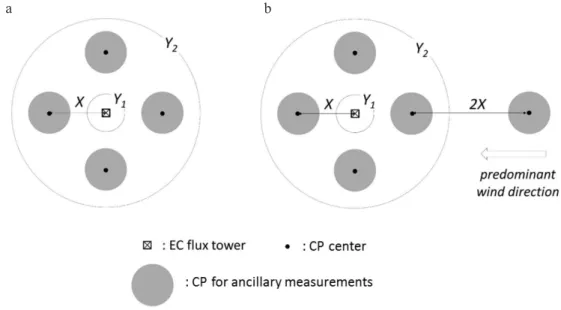
The organisation of the plots, for forest and cropland stations, in its most rudimentary form, is described in the basic sampling design. With this approach, N continuous plots (CPs) are systemically arranged around the EC flux tower. The number of plots differs between the two classes of monitoring intensity that are defined within the ICOS ecosystem network: N = 4 (+ 1 optional) at Class 1 stations; N = 2 at Class 2 stations (Fig. 1). A CP is a non-fenced area where the ancillary measurements are carried out. The plot is the statistical unit of spatial replication: at each sampling date, the ancillary variables are measured in each plot. Site averages and standard deviations are calculated on the basis of plot values – a single value per plot. The CP also com-prise the soil meteorological measurements, ideally located in the center of the plot. The locations of the ancillary and soil measurements are matching in order to facilitate assessments of spatial variability in ancillary variables in relation to spatial variability in soil climatic conditions.

Measurements in these plots are repeated throughout the growing season to address temporal variability.

• The four plots at Class 1 Stations are located at a distan- ce X from the EC tower, which is set at15 m for croplands and 35 m for forests, following a cross-like design (at 90°

increments starting from the prevailing wind) (Fig. 1a). If a predominant wind direction prevails, an optional fifth plot can be installed further upwind from the EC tower (Fig. 1b).

• The two plots at Class 2 stations are located at the two positions in the cross-like design that are deemed most rep-resentative for the area measured by the EC system.

This basic sampling design is a minimal design that defines the location and number of plots around the EC tower for a generic ICOS forest or cropland station with a homogeneous vegetation cover. This design is adapted for each single station with vegetation-specific modifications and station-specific adjustments to differences in vegeta-tion heterogeneity in the target area.

Modification to the general design

The location of the plots can be adjusted if they fall in areas that are not representative of the vegetation within the target area or cannot be used due to access restrictions. The locations should be selected striving for maximal rep-resentativeness of the vegetation within the target area. Distances vary between 30 and 100 m for forests, and to 10 and 35 m for croplands (Fig. 1).

Measurements inside the continuous plots

Measurements of GAI and AGB through destructi- ve sampling are carried out in at least two locations (fol-lowing the description below) within each continuous plot.

Fig. 1. The basic sampling design for ancillary measurements in forest and cropland stations. a – At Class 1 stations, four Continuous Plots (CP) for ancillary data measurements are located around the EC flux tower following a cross-like design. At Class 2 stations, two CP are located at the two positions in the cross-like design that are deemed most representative for the target area. b – At Class 1 sta-tions, an optional fifth plot is installed further upwind from the EC tower in case of a predominant wind direction. The default distances (X) between the tower and the center of a plot vary per ecosystem type: X is set to 15 m for croplands and 35 m for forests The range of the distance where the plot can be relocated is set between 10 m (Y1) and 35 m (Y2) for croplands and 30 m (Y1) and 100 m (Y2) for forests.

The amount of sampled vegetation at each location will vary with crop and cultivation method:

• row crops:

o if plants are uniformly spaced in the row: at least six neighboring plants in one row or 2 x 3 neighboring plants in twin rows (Fig. 2a; e.g. maize, sugar beet, potato, sunflower),

o if plants are irregularly spaced in the row: at least 1 m of row (Fig. 2b; e.g. wheat, barley, oilseed rape), • single-spaced large crops: at least two neighboring plants

(Fig. 2c; cabbage, broccoli… ),

• broadcast sown crops: all plants rooting within a 0.5 x 0.5 m quadrat (Fig. 2d).

The harvested material is split into the following fractions:

•

•

•

•

•

Harvested areas can be chosen in all directions but must be at a distance at least three times the maximum seasonal crop height from other harvested areas and from locations where GAI is measured indirectly. If needed, the quadrat area in broadcast sown crops should be increased to include at least five crop plants.

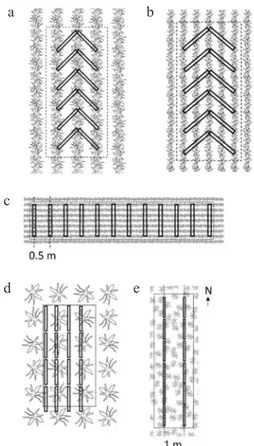
Ceptometer measurements of GAI are carried out at a minimum of three locations in each plot. At each loca-tion, measurements of below-canopy PAR (PARb) are done

with the ceptometer probe as shown in Figs 3 and 4, while above-canopy PAR (PARa) is simultaneously measured with

the external PAR sensor installed nearby. The positions of the below-canopy measurements will vary with crop arrangement:

• row crops: 12 PARb measurements along two

paral-lel transects that follow the direction of the rows. The ceptometer probe is held diagonally to the row, extending from row to row, and depending on row distance, spanning

one or more rows (Fig. 3a-b). When row distance is small (<10 cm), the probe is held perpendicular to the rows and a measurement done every 0.5 m (Fig. 3c).

• single-spaced large (>1 m) crops: 12 PARb measure-

ments along transects parallel with row direction, alterna- ting between rows and within the rows. At least 4 x 2 indi-vidual plants are included (Fig. 3d).

• broadcast sown crops: 12 PARb measurements along

two parallel north-south oriented transects, spaced 1 m apart (Fig. 3e).

Fig. 2. Vegetation sampled at each location: a – row crops with uniform plant spacing in the row, b – row crops with irregular plant spacing in the row, c – single-spaced large crops, d – broadcast sown crops. The plants that need to be harvested are highlighted.

a

c d

b

Fig. 3. The position of below-canopy measurements at each loca-tion for different crop arrangements: a and b – row crops, c – row crops with narrow rows, d – single-spaced large crops and e – broadcast sown crops. Dotted rectangles show the area that has to be sampled destructively for the once-per-season comparison of ceptometer measurements with directly measured GAI.

a

c

d e

The measurement locations must be at a distance of at least three times the maximum seasonal vegetation height away from other locations and from areas in the plot that are destructively sampled. The locations are fixed, which means that the measurements are repeated on the same veg-etation throughout the season. The locations are selected based on the representativeness of the vegetation by the sta-tion PI at the first GAI measurement of the season and then their positions are marked (e.g. with a plastic tag) so they can be revisited. If vegetation is destroyed in the season, then a new location must subsequently be selected.

Temporal sampling design

The measurements of GAI, AGB, and litter are com-bined in a single temporal sampling scheme.

Measurements of GAI are carried out regularly during the growing season in order to assess seasonal variations They should be timed to include both the maximum and minimum variability in seasonal GAI.

Between crop emergence/planting and harvest, GAI is measured:

• once at each of the six selected developmental growth stage of the crop (crop species specific),

• once just before harvest,

• after a major disturbance, such as a storm event.

Between two crop seasons, GAI is measured only if the field is vegetated, e.g., with a cover crop, voluntary regrowth or abundant weeds (with a minimum vegetation cover of 10%), on a monthly basis.

The developmental growth stages of crops are defined and coded following the BBCH-scale as described by Meier et al. (2009). The selected stages are specific for each major crop species. Expressing the timing of the measurements as a function of crop development, rather than following a fixed time schedule, enables the matching of the temporal sampling to species and site.

Calibration measurements for the indirect method are carried out on a selection of the destructive AGB samples at peak biomass.

AGB is determined:

• once at the seasonal maximum AGB, if occurring before harvest,

• once at harvest,

• after each major disturbance, such as a storm event (to be judged by the PI; these could be events that occur only once every 5 years which result in a reduction in AGB), • once between two crop seasons if the field is vegetat-ed: at the AGB peak of cover crops (timing based on PI judgement), voluntary regrowth or significant weed populations.

When GAI and AGB measurements coincide and both variables are determined from destructive sampling, they are determined using the same material.

Litter biomass is measured:

• with maximum intervals of 14 days (this frequency is needed because litter needs to be collected before any significant decay),

• once at (or right before) harvest,

• monthly between the two crop seasons if the field is vege- tated, e.g., with a cover crop or abundant weeds,

• after harvest, to estimate residues inputs, and after major disturbance events (e.g. droughts, storms).

The litter should be collected regularly to reduce any leaching and decomposition losses, although more frequent collections are recommended for litter types that decom-pose rapidly and when there is a high-rainfall or windy conditions.

Harvest residues should be collected directly after harvest.

Grassland stations

Methods to measure GAI, AGB and litter biomass measurements

Destructive measurements and ceptometer

The description of the destructive measurement method and the indirect ceptometer measurements for grasslands is similar to that used for croplands and thus can be found above.

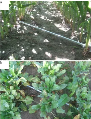
Fig. 4. Example of a below-canopy probe position in: a – a maize crop and b – a beet crop.

a

Indirect methods – the plate meter

A plate meter is a simple instrument that basically con-sists of a graduated stick stuck through a centered hole in a plate with a certain weight. A measurement with the plate meter involves lowering the plate until it is supported by the vegetation. The height of the plate resting on the vegetation is a combined measurement of the height and density of the compressed vegetation beneath it. This height can be lin-early related to AGB, and also to GAI given that the ratio of green-to-total biomass is fairly constant over the grassland site. As mentioned before, the height of the plate is simply referred to as bulk height. The advantage of the plate meter is that it requires minimal effort to collect many measure-ments of bulk height, from which GAI and AGB can be inferred with established relationships between bulk height and directly measured assessments of GAI and AGB. Since these relationships are affected by changes in the structure and composition of the vegetation, they have to be updated repeatedly throughout the growing season.

Litter biomass and harvest residues

Litter biomass and harvest residues in grasslands are measured by collecting all litter and residues on a given area at AGB measurement plots. After cleaning the col-lected material to remove soil particles and other non-plant material. Values for litter biomass or harvest residue are obtained by dividing the total dry weight with the sampled ground surface area.

The ability to adequately assess litter biomass in all grasslands varies. For instance, compare a dry grassland where litter can be easily collected from the hard soil sur-face with a wet, grazed grassland where intensive treading by livestock mixes the litter with the muddy surface layer of soil. In the latter case, it is virtually impossible to obtain good measurements of litter biomass. In such situations, lit-ter biomass should not be measured, acknowledging that this may introduce significant errors in the estimation of yearly ANPP. The station PI is responsible to judge whether litter biomass measurements at individual grassland sites are appropriate. Litter and harvest residues do not need to be separated between plant functional types.

Spatial sampling design

In contrast to the continuous sampling plots that are used for cropland and forest ecosystems, the ancillary vege- tation measurements in grasslands are organized using the sparse measurement points, which are defined in the target area at the start of ICOS term as described in Saunders et al. (2018).

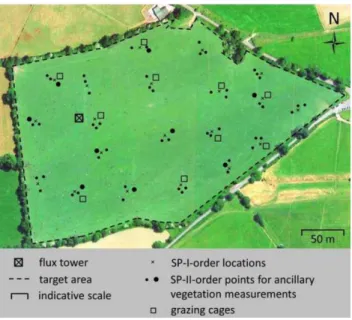
At each measurement date, 60 sparse measurement (SP-II order) points are selected, i.e. three SP-I-order points around each of the 20 SP-I-order locations. The points can be selected considering all the SP-II locations communi-cated by the ETC, i.e. both the 5 main points and the 15 reserve points. From these 60 points, a small subset of N

points is selected (see example Fig. 5), with N being a sta-tion-specific value determined as explained further below. The measurements are carried out at the selected points as follows:

• AGB and GAI values for all 60 points are estimated using the relation between bulk height and destructively measured values for GAI and AGB, respectively. The aver-age GAI and AGB for the target area then derived from relationships between bulk height and GAI and between bulk height and AGB.

• If it is opted to measure GAI with the linear ceptom-eter, GAI is measured with the ceptometer at all 60 points. In this case GAI is not measured directly by destructive sampling at the N points (while AGB is), except once per growing season. This once-per-season measurement has to be done near or at a GAI peak. It is done for comparison/ validation of the ceptometer measurements with directly measured GAI.

• Litter biomass measurements are done on litter mate-rial collected at the N points.

• Stubble measurements are done at another set of N SP-II-order points in a designated part of the target area where vegetation is representative for the target area. This is discussed and agreed between the station PI and the ETC.

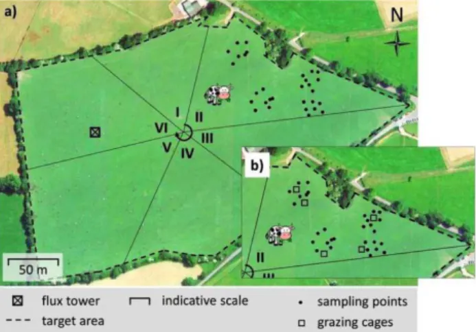
Fig. 5. Spatial sampling scheme. At each measurement date, 60 order points are selected (all black dots), i.e. three SP-II-order points around each of the 20 SP-I-SP-II-order locations (crosses). From these 60 points, a subset of N points is selected (large black dots). In this example N = 10. If the target area is grazed, grazing cages are additionally installed at the start of the grazing period at another 10 and 5 SP-II-order points in Class 1 and Class 2 stations, respectively (squares). For an explanation of what is measured at each point and in each grazing cage, see main text. Note: points for stubble measurements and points for harvest residue collection are not shown in this figure.

If the target area is grazed, exclusion cages are installed in the target area at the start of the grazing period: 10 cages at Class 1 stations and 5 cages at Class 2 stations. Cages are installed at SP-II-order points other than the 60 selected points. At the end of the grazing period, bulk height is measured with the plate meter in each cage for estimation of AGB, which is needed to estimate grazed biomass. In at least two cages, AGB is also measured by destructive sampling. The latter measurements yield points that are added to the dataset from which a relationship between AGB and bulk height is derived. If needed, the cages are relocated during the grazing period.

If the target area is cut, harvest residues are collected after each cutting event at another set of N SP-II-order points.

At each measurement date, the SP-II-order points for measurements are selected by the station PI from all SP-II-order points in the following way:

• To select a set of 60 SP-II-order points, randomly select per SP-I-order point three SP-II-order points. If a se- lected point is unsuitable for the measurements, take the next available point. For example, if point SP-II_01-04 is unsuitable, take point SP-II_01-05. If also this point is unsuitable, take SP-II_01-06, and so on. A point is unsuit-able for the measurements when it has been destructively sampled earlier in the current or previous growing season. If the point has been sampled for stubble, even if this sam-pling was done more than two seasons ago, the station PI should determine whether the vegetation at that point has regrown sufficiently and a representative measurement can be done at that point.

• To select a subset of N points for destructive sam-pling/litter collection, randomly select N points from the 60 selected points. Each of the N points has to belong to a unique SP-I-order point. So if two (or more) points around a same SP-I-order point are selected; only keep the first point, and randomly select one (or more) other points. Repeat if needed.

• To select N points for stubble measurements, random-ly select N points from all SP-II-order points available, i.e. from all points except the 60 selected points. Each of these N points has to belong to a unique SP-I-order point.

• To select N points for harvest residue collection, ran-domly select N points from all SP-II-order points available. Each of these N points has to belong to a unique SP-I-order point.

• To select points for grazing cages, select N points from all SP-II-order points available. Each of these points has to belong to a unique SP-I-order point.

The random selection of points can be done by means of a random number generator in Excel, or by simply drawing lots from a bag, etc. The value for N is station-specific and determined from direct AGB measurements performed at the beginning of the station operation in the context of the site characterization. A value for N is calculated from the

AGB data as being the minimum number of direct meas-urements needed to determine the mean AGB of the target area within a desired margin of error set by the ETC. The calculated value is applied from the second year of ICOS measurements, while for the measurements in the first year N is fixed to 10 for Class 1 stations and 5 for Class 2 sta-tions. These values are valid for all numbers mentioned above that are denoted as ‘N’.

Measurement at each sampling point: Destructive measurements

Destructive sampling is to determine AGB and GAI done by sampling a square quadrat with a minimum size of 25x25 cm. The station PI determines a site-specific quadrat size on the basis of the density and structure of the vegetation. In grasslands with sparse and heterogeneous vegetation, larger quadrat sizes are required than in grass-lands with dense, homogeneous vegetation. In row-sown grasslands with clear rows, the size of the quadrats is cho-sen such that the quadrats span an integer number of rows. The same quadrat size is used at all sampling points and at all measurement dates in the growing season. It is also the quadrat size for the destructive measurement of stub-ble. The harvested green material is split into legumes and non-leguminous so that GAI can be determined separately.

Ceptometer measurements

At each SP-II-order sampling point, measurements of below-canopy PAR are done with the ceptometer probe at three parallel, north-south oriented probe positions spaced 40 cm apart as, while above-canopy PAR is measured simultaneously with the external PAR sensor. In row-sown grasslands with clear rows, the probe is positioned between rows and the distance between the probe positions is hence adjusted to the distance between rows.

Plate meter

Measurements are done with a square plate having the same dimensions as the sample quadrat for destructive samplings.

Litter collection

Litter collection is done by collecting all litter in the sampling quadrat after clipping the vegetation. Collection of harvest residue in cut grasslands is done in a large 4x4 m square quadrat at each SP-II-order sample point.

Stubble measurement

A stubble measurement is done by first installing the same metal grid that is used for destructive sampling at all SP-II-order sampling points and then clipping the vegeta-tion in the quadrat back to stubble height. The stubble is then clipped down to the ground. The collected stubble material is rinsed with water to discard adhering soil par-ticles and other non-plant material. Green Area Index and

AGB of the stubble are then determined as described in the destructive sampling procedure. Stubble should however not be separated between plant functional types.

Temporal sampling design

The ancillary variables have to be measured repeatedly throughout the growing season. Minimum requirements include a measurement at the start and the end of the grow-ing season and a measurement at each peak and trough of GAI/AGB within the growing season. The latter implies in agricultural grasslands a measurement immediately before and after each cutting (= max. 3 days), with “natural” lit-ter biomass only measured immediately before the cutting and harvest residue biomass obviously after the cutting. In case of grazing, it implies a measurement at the start and the end of each grazing period. In those cases where the measurements prescribed above appear too rare, additional

measurements in between are recommended for good tem-poral coverage. This can be the case for a grassland with one vegetation peak (Fig. 6a) or with a long grazing period (Fig. 6b). The absolute minimum measurement frequency for any station is five measurements per year. The maxi-mum period of time between two measurements is very much dependent on the growth dynamics of the vegeta-tion but, as a general rule, set to three to four weeks. In agricultural grasslands, the measurement immediately after a cutting late in the season or the measurement at the end of a grazing period that is timed late in the season can sub-stitute for the normal end-of-season measurement. This should be agreed with the ETC, considering also the esti-mated end-of-season contribution of the vegetation to the yearly ecosystem fluxes. Stubble measurements are done three times per year: at the start, middle, and end of the growing season.

Fig. 6. Examples of the timing of measurements in the growing season: a – in a grassland that is neither cut nor grazed and with one vegetation peak in the growing season; b – in a grassland that is first cut and later grazed. In this example, grazing cages are relocated once in the grazing period. See main text for a detailed explanation. Note: litter biomass should be measured only before a cutting.

a b GAI GAI AGB litter biomass AGB litter biomass Time

Additional measurements for estimation of harvest biomass If the target area of a grassland site is cut, harvest residues are measured immediately after machine collec-tion of the cut biomass. The seasonal patterns shown are hypothetical: it is assumed for simplicity that there is no decomposition of biomass and that litter accumulates in the course of the growing season as biomass dies off. It is up to the station PI to refine the timings to the vegetation dynam-ics and the scheduled management activities at the site. Additional measurements for estimation of grazed biomass

If the target area is grazed, grazing exclusion cages are installed at the start of each grazing period. The above-ground biomass in the cages is assessed (from bulk height) and a destructive harvest at the end of the grazing period is carried out, which coincides with a measurement of GAI, AGB, and litter in the grazed target area (Fig. 6b). For longer grazing periods, the AGB of the vegetation in the cages should also be assessed during grazing and the cages subsequently relocated. This is to avoid systematic underestimation of grazed biomass that might result from the fact that the taller vegetation in the cages tends to grow slower than the short grazed vegetation outside the cages. For each relocation should coincide with a measurement of GAI, AGB, and litter biomass in the target area. To determine regrowth, some cage locations are cut prior to relocation and regrown biomass is added to the biomass obtained from cages which have not been cut before. The exact timing of these measurements is at the discretion of the station PI.

Rotational grazing systems

For grazed sites, sampling for the estimation of grazed biomass with cages applies only when the grazers roam one pasture spanning the target area. The sampling is dif-ferent for rotational grazing systems where the target area is divided into paddocks and the animals are moved from one paddock to the next every few days to weeks (Fig. 7).

While measurements of GAI, AGB, and litter biomass in these rotationally grazed systems are carried out follow-ing the samplfollow-ing design explained above, the estimation of grazed biomass requires AGB to be assessed in each pad-dock every time it is grazed. This is done on the basis of bulk height measurements.

• If the grazing time in each paddock is short enough to assume no significant regrowth during grazing, which is typically a few days at maximum, grazed biomass is simply assessed from the difference in AGB before and after graz-ing. Here, bulk height is measured with the plate meter at a minimum of 30 randomly selected points in the paddock just before the grazers enter the paddock and immediately after the grazers are removed from the paddock (Fig. 7a, Fig. 8a).

• If the grazing time in each paddock is long enough to expect significant regrowth of the vegetation during graz-ing, the grazed biomass is assessed from the difference in AGB between the vegetation accessible to the grazers and the vegetation inside the cages. For this, at least five cages are installed just before the grazers enter the paddock. After the grazers are taken away from the paddock, bulk height is then measured with the plate meter inside the cages and for a minimum of 30 randomly selected points in the paddock (Fig. 7b, Fig. 8b). A further 5 cages are installed to deter-mine regrowth, and the vegetation is cut prior to installation and regrown biomass is added to the biomass of the cages which have not been cut previously.

Estimates of AGB can be made using bulk height meas-urements. The relationship between the two variables is assessed from the direct AGB measurements and the bulk height measurements for a subset of N sampling points in the target area at each measurement date for GAI and AGB. As this relationship is affected by the changing vegetation structure during the grazing period, it is updated at each measurement date, or more often, if needed, from addition-al measurements.

If the target area is cut, harvest residues are measured immediately after machine collection of the cut biomass. Figure 8 shows graphical examples of the temporal sampl- ing scheme. The seasonal patterns shown are hypothetical: it is assumed for simplicity reasons that there is no decom-position of biomass and that litter accumulates in the course of the growing season as the vegetationdies off. The given numbers of measurements represent the absolute mini-mum and the timings are indicative. It is up to the station PI to refine the timings to the vegetation dynamics and the scheduled management activities at the site.

Fig. 7. Example of the sampling during rotational grazing in grasslands. Shown are only the measurements needed for grazed biomass estimation in one paddock: a – if the grazing time in each paddock is very short, b – if the grazing time in each paddock is long enough for significant regrowth during the grazing. See main text for explanation.

Forest stations

Methods to measure PAI, AGB and litter biomass For forest ecosystems digital hemispherical canopy photography (DHP) and the ceptometer are considered standard methodology to estimate PAI at the ICOS stations.

Hemispherical photography is a technique that is used to study plant canopy structure via photographs acquired through a combination of a camera and hemispherical (fisheye) lens from upward or downward looking digital hemispherical pictures. These pictures provide a permanent record and therefore a valuable source of information to assess canopy structural properties. This technique is able to capture species-, site- and age-related differences in can-opy architecture, based on light attenuation and significant contrast between features within the captured image (sky versus canopy). Hemispherical photographs generally pro-vide a very large (close to 180°) field of view; in essence, they produce a projection of a hemisphere on a plane (Rich, 1990). The exact nature of the projection varies according to the properties of the hemispherical lens. The simplest and most common hemispherical lens geometry is known as the polar or equi-angular projection (Herbert, 1986; Frazer et al., 1997). The most critical step in image pro-cessing is probably determining the threshold between the sky and canopy elements. Estimations of PAI are based

on the angular, zenithal and azimuthal, distribution of gap fractions (visible sky) after image thresholding. Random distribution of canopy elements within the canopy volume is generally assumed (Jonckheere et al., 2004; Weiss et al. 2004). Thus DHP is an optical method that enables rela-tively accurate, fast, and sequential measurements of PAI at the plot scale. This technique can further help to estimate useful attributes of canopy structure other than PAI, such as canopy openness or canopy cover and foliage clump-ing and is very useful for characterizclump-ing below canopy light microclimate (Walter et al., 2003; Gonsamo and Pellika, 2009; Whitmore et al., 1993). Due to the risk of saturation of the PAI retrieved with DHP in forests with a PAI value higher than 6 m² m-2_{, we recommend for those stations}

that the ceptometer-based approach is used, where above and below canopy light levels are measured independently from each other (for a description of the ceptometer method see the section on measuring GAI in croplands).

To allow sequential measurements in permanent plots, the recommended methodology for AGB estimations in forests is the use of allometric techniques while the AGB of herbaceous vegetation in the understory should be meas-ured using destructive sampling. Allometry involves the estimation of woody biomass from size parameters that are relatively easy to measure. The woody biomass of a tree can be inferred from stem diameter at 1.3 m, hereafter

GAI _AGB

litter biomass

Fig. 8. Example of the sampling design in a grassland that is first cut and then divided into six paddocks for rotational grazing. Target area-representative measurements of GAI of AGB are done throughout the growing season following the sampling design illustrated in Fig 6a, but for the estimation of grazed biomass, AGB has to be measured in each paddock every time it is grazed; a – example with a grazing period of four rotation cycles and grazing times in each paddock that are short enough to expect no significant regrowth of vegetation during the grazing; b – example with a grazing period of one rotation cycle and grazing times in each paddock that are long enough to expect significant regrowth of vegetation during the grazing. See main text for a detailed explanation.

a b

referred to as diameter at breast height (DBH), and tree height. Wood and foliage biomass of shrub species is often calculated from measurements of basal stem diameter and crown dimensions. Biomass values for a given plot area are obtained by measuring all trees or shrubs growing within the plot together with the application of species-specific – and preferably also site-specific – allometric equations. Destructive measurements on individual plants from differ-ent size classes provide the data needed to parameterize and validate the allometric equations. All Class 1 forest stations should measure allometric relations for each of the species that cover a minimum of 80% of the basal area within their continuous measurement plots.

Exceptions to this approach are allowed when existing allometric relations are available from the literature with: 1) mean annual temperatures within 2°C of the research

station

2) mean annual precipitation within 200 mm of the research station,

3) similar soil type,

4) age class within a 30 year range of the mean stand age currently present.

Within each species, trees should be selected so that all size classes are measured. Class 2 stations should also use site-specific allometric relations if they are available from previous sampling campaigns. Alternatively, a multitude of allometric relations have been published in recent years (Albaugh et al., 2009; Muukkonen and Mäkipää, 2006; Muukkonen, 2009; Wirth et al., 2009; Zianis et al., 2005), which can be used when site-specific allometric relations are not available.

Litter biomass is measured simply by collecting litter with litter traps installed beneath the vegetation. The non-woody litter that is captured in litter traps or located within the boundaries of a sampling plot is collected at least bi-weekly within the main period of litter fall, to prevent the onset of decay. Outside this main period the traps should be emptied at least every month. The litter should be separated into the different fractions: branches (<2 cm), leaves, fruits and flowers. The leaves should be separated at species level. The collected litter material should be dried until constant weight is achieved (65°C, usually 24-48 h). A value for lit-ter fall is obtained by dividing the total dry weight with the collecting area of the litter traps or the ground surface area of the collection plot.

The pool of fine woody debris is measured using fixed collecting plots of 1 by 1m on the forest floor, while coarse woody debris is commonly measured using line intersect sampling (Warren and Olsen, 1964). The latter technique measures all diameters of the woody debris, along a tran-sect in the forest. These diameter measurements, combined with estimates of the decay class, allow us to estimate the coarse woody debris pool in an efficient way. This tech-nique is currently used by large forest monitoring networks (Woodall and Williams, 2005).

Spatial sampling design

The general spatial sampling design for the forest sta-tions is described in the croplands section (see above). Measurements inside the continuous plots

For forest ecosystems a CP is a circular measuring plot with a fixed radius of 25.24 m (surface 2 000 m²) where, at the centre of each CP instruments measuring soil tempera-ture, soil moisture and soil heat flux and water table depth are located.

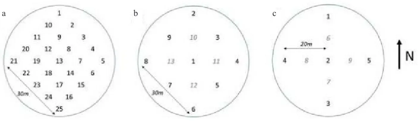
Measurements with the ceptometer are carried out at 25 locations in the CPs. At each location, below-canopy PAR (PARb) is measured with the ceptometer probe, while

above-canopy PAR is measured simultaneously with the external PAR sensor installed in a nearby clearing or on the EC tower. A systematic measuring grid has to be installed within each CP. For a standard circular CP, a grid of 25 points must be used with 7.5 m between points and with the middle point (ID = 13) coinciding with the center of the CP (Fig. 9a). The four corners of the square have to be at equal distance from the center of the plot, with the upper one fac-ing north. To avoid interference from stems and trees we advise moving the measurement point away from a tree using the 10° rule that implies that a sampling point should be at a minimum distance of 5.7 times the diameter of the tree. In practice this can be easily checked by constructing a stick in the form of a T, where the long end is 5.7 times longer than the short end. When pointing this device toward a tree the width of the tree should be less than the short end of the T device. Thus, this device could be used to decide if trees are too close to the measuring point. In cases where the sampling point is too close, the point should be moved away from the tree in any direction. Once a point is deter-mined it has to be kept constant over the lifetime of the ICOS ecosystem station.

When measuring for the first time, the measurement locations should be marked with a wooden/metal stick with a clear tag on it.

For the DHP determinations, a systematic measuring grid of nine points has to be installed within each CP. In a standard circular CP, the points are 15 m from each other with the middle of the systematic grid collocated with the centre of the plot (Fig. 9b). The four corners of the square have to be at equal distance from the centre of the plot, with the upper one facing north. An additional four measure-ment points might be added in agreemeasure-ment with the ETCif the standard error of the PAI within the plot is larger than 5% of the mean. To avoid interference from stems and trees on the measurements we advise moving the measurement point away from a tree using the 10° rule where the sam-pling point should be at a minimum distance of 5.7 times the diameter of the tree (see ceptometer measurements). The minimum distance between the lens and a leaf has to be 10 times the length of the leaf. Thus in the case of a leaf of length 10 cm, the minimum distance to the lens has to be

100 cm. Leaves that are too close for their size have to be removed. When sampling for the first time, mark the meas-urement location with a wooden/metal stick with a clear tag. Each location must be marked with an ID following the scheme in Figure 9b that will be required for data submis-sion. Measure the mean terrain slope and slope direction of the CP, considering the full area covered by the CP.

Diameter at breast height (DBH) should be measured for all trees in the CP with a DBH larger than 5 cm. A girthing tape is preferred over the (digital) caliper for measurements on tree stems. A girthing tape measures circumference, integrating stem diameter in all radial directions and elimi-nating diameter variability caused by direction when the stem shape deviates from circularity. When using a caliper, two measurements have to be taken, perpendicular to each other. The average of the two has to be noted. In addition, also the height of the tree, the species and the health status should be noted. The health status is divided into four main categories that are judged by the operator.

One of the following four categories have to be assigned to a tree (healthy, with minor diseases, or with major dis-eases, or dead) and each category is defined as:

1) Healthy: no visual indication of the crown being affected by diseases, herbivory, storm damage. Damage is defined by branches that lost leaves or where leaves have changed colour.

2) Minor diseases: visual indication of the crown being affected at maximum 50% by diseases, herbivory, storm damage.

3) Major diseases: visual indication of the crown being affected ≥ 50% by diseases, herbivory, storm damage, but still healthy leaves are present.

4) Death: the tree contains no more visibly living branches and leaves.

To calculate AGB, tree height measurements are need-ed. Tree height is the vertical distance between the highest point of the crown and the ground surface. Measurement of the tree height is based on the relationship between the

horizontal distance from a point to the tree stem base and the angle from the point to the stem base and tree top. These measurements can be achieved using laser distance meters and an inclinometer. To reduce the error in the measure-ments of the angle, the point from which it is measured must be as far from the tree as the tree is high.

Forest understorey

The aboveground biomass of saplings (DBH <5 cm) and shrubs have to be included in the understorey assess-ments, together with the herbaceous vegetation.

The AGB of the understorey vegetation has to be meas-ured by destructive sampling (herbaceous vegetation) and the use of allometric relations (saplings and shrubs) in five predefined harvest plots of 0.25 x 0.25 m for the herba-ceous vegetation (destructive) and five predefined 1 x 1 m plots for the saplings and shrubs (non-destructive), all within each CP. The location of the plots will be randomly assigned by the ETC.

Litter biomass

Non-woody litter biomass is measured using litter traps that are installed in each CP. The minimum collecting area of the litter trap is 0.5 m² (radius = 0.39 m). A minimum of five locations must be used, positioned in a cross like design (Fig. 9c), where the distance between the litter traps on the axis is 20 m and where the central litter trap coincides with the centre of the CP. There is the possibility to add four additional traps located exactly in between the existing lit-ter traps with a distance of 10 m. The ETC will evaluate the need for this additional installation after the first year of measurements. In the field all the material from each litter trap is collected in separate bags ensuring the bag contains the ID from the litter trap and the ID of the CP. All branches with a diameter larger tha 2 cm should be removed from the collected material. After this the following fractions should be separated and weighed: twigs smaller than 2 cm, leaves, fruits, flowers.

Fig. 9. Spatial sampling design for forest stations for measurement inside one plot for: a – ceptometer, b – digital hemispherical pictures c – and the litter traps. The numbers indicate the regular sampling locations and the additional sampling location (light grey).

Temporal sampling design

Determinations of GAI are made for the canopy and the woody understorey if present:

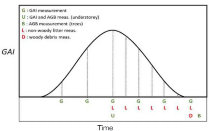
• at least six times a year (Fig. 10) for both deciduous and coniferous forests, depending on the species: two times at the onset of leaf development, once at the peak GAI, two times between the peak GAI and senescence and a final measurement during the dormant season,

• in addition, once just before and after thinning, • after a major disturbance, such as a storm event; for the herbaceous understorey:

• once a year near peak GAI of the understorey vegetation. The frequency of AGB is determinations are made: • once every three years for standing woody biomass

(trees) within the continuous plots, during the dormant season,

• once every year for the understorey vegetation (prefer-ably at peak biomass for non woody vegetation), • after each major disturbance, such as a storm event, • continuously for standing woody biomass using

automat-ic dendrometers (Class 1 Stations only).

• In addition, the amount of material removed at harvest has to determined.

The AGB sampling of the herbaceous understorey veg-etation is integrated into the GAI sampling schedule for the herbaceous understorey.

Non-woody litter should be measured:

• with a maximum interval of two weeks during the period of main litter fall and monthly outside this period. This will depend on the seasonal pattern of leaf or needle fall for the specific species present at the station. The fre-quency will also depend on the likelihood of decay • once at (or right before) harvest,

• after a major stress event (e.g. drought, storm).

The litter should be collected regularly to reduce leach-ing and decomposition, although more frequent collections are recommended for litter types that decompose rapidly and under high-rainfall conditions. Fine and coarse woody debris is measured each year, preferably at the same time of the year

Mire stations

Methods to measure GAI and AGB

Measurements of GAI and AGB are made using indi-rect methods in permanent plots within the target area. Measurement methods are described here for mosses, her-baceous vascular plants, and dwarf shrubs. The selected methods for each plant functional type (PFT) are listed in Table 1. They are favoured over other indirect methods because they allow GAI and AGB to be determined at the level of the species and the PFT, which is useful for iden-tifying changes in ecosystem fluxes and yearly ANPP that are due to shifts in vegetation composition.

The calibration of the selected methods is done on the basis of destructive samplings in the first ICOS measure-ment year and regularly thereafter. Should stands of trees be included in the target area, then ancillary measurements of the trees are carried out following the methodologies described for forest ecosystems. Also, should grasses/ grassland-like vegetation, rushes, etc. be included in the target area GAI and AGB should be measured following the methodologies described for grassland ecosystems.

The Green Area of mosses is the fraction of the ground surface area covered by living moss capitula. Green Area is estimated visually in quadrats of 60 cm x 60 cm (e.g. Fig. 10. Default scheme of the temporal sampling for ancillary

vegetation measurements at forest stations. Note: understorey GAI and AGB is measured at peak of herbaceous species GAI.

Time

T a b l e 1. Selected methods for each plant functional types (PFT) at wetland stations. VGA = Vascular Green Area Index

PFT GAI AGB or biomass increase*

Mosses Green Area_{(visual estimation)} the brush wire method*

Herbaceous vascular plants (include

grasses, sedges, rushes, and forbs) the VGA method the VGA method 1

Dwarf shrubs the VGA method non-woody: the VGA method

1 woody: the modified point intercept method

Leppälä et al., 2008; Riutta et al., 2007a) and can be aided by using a frame divided into sub-quadrats (e.g. 10 x 10 cm). The estimated moss cover in each sub-quadrat is added together to obtain the total cover in the quadrat.

The brush wire method (Clymo, 1970; Granath and Rydin, 2013) is used to measure moss growth biomass increase. With this method, the length increase of moss stems is measured against an external reference, these are the brush wires inserted in the moss layer at the start of the growing season. The brush wires are pushed into the moss layer, parallel to the stems and extending above the moss carpet. The moss grows up around the free end of the wire and length growth is measured from the distance change between the moss tip and the tip of the brush. Concomitantly, the density of living moss stems is deter-mined by counting the number of living stems per unit of ground surface area. Moss growth biomass increment is obtained from the length growth, moss stem density, and a value for the dry mass of moss stems per unit of stem length. The latter is obtained from destructive samplings.

For herbaceous vascular plants and dwarf shrubs GAI is derived with the vascular green area index (VGA) method (Wilson et al., 2007), based on measurements of the number and the size of leaves and stems. The method involves counting the number of green leaves and stems of all individuals of a given species found inside a quadrat. Concurrently, the size of all leaves and stems of a few indi-viduals outside the quadrat is measured (e.g. length, width, diameter). From these measurements, leaf and stem areas are calculated with a geometric formula that relates area to size. The GAI for a given species is then obtained by multiplying the total counted number of green leaves and stems with the average leaf and stem area and expressing the results per unit of ground surface area.

For dwarf shrubs with numerous, tiny leaves that are hard to measure individually, an alternative allometric method is used. Instead of measuring the number and area of single leaves, the total length of green stems covered by leaves is measured. In this case GAI is derived with values for the area of leaves per unit of stem length obtained from destructive samplings.

The estimate of AGB of herbaceous plants and the bio-mass of non-woody aboveground parts of dwarf shrubs for each species are derived from GAI calculated with the VGA method at the seasonal GAI peak. Area is converted to biomass by applying area-to-biomass ratios for leaves and stems obtained from destructive samplings.

This measurement of (green) AGB is a direct estimate of the yearly ANPP for herbaceous plant species if we can assumethat all green plant material has been produced in the current growing season, that no new material is pro-duced after the GAI peak, and that no senescence has occurred before the GAI peak. Similarly, this measurement is a direct estimate of the non-woody fraction of yearly ANPP for dwarf shrub species.

For the estimation of the woody AGB of dwarf shrub species (i.e. stems) the modified point intercept method (Jonasson, 1983, 1988) is used. It is a variant of the point intercept method for plant cover estimates to make it appli-cable for biomass assessments. With this method, a thin needle is passed through the vegetation vertically at regu-larly spaced positions within a quadrat. The total number of times that the needle hits a woody stem of the given species is counted. Woody stem biomass can then be derived from the total number of hits with regressions fitted to data of destructive samplings of woody stem biomass versus the number of needle hits.

Spatial sampling design

Mire vegetation is often comprised of various plant community types that contribute differently to the ecosys-tem GHG fluxes (e.g. Alm et al., 1997; Bubier et al., 1993; Granberg et al., 1997) and that are distributed in accordance with the mire’s (micro)topography and the associated mois-ture gradient (Rydin and Jeglum, 2013). The measurements are therefore organized following a stratified sampling design: the mire vegetation inside the target area is divided into plant community types with each plant community type contributing significantly to the measured ecosystem fluxes, and GAI and AGB are measured in a number of per-manent plots located inside the target area. In these plots measurements are repeated periodically to assess the sea-sonal pattern of GAI and AGB.

The classification of the mire vegetation into plant com-munity types should be done on the basis of an analysis of the results of a systematic vegetation survey (such as done in e.g. Maanavilja et al., 2011; Malmer et al., 2005; Riutta et al., 2007b). This survey is part of the vegetation charac-terization, which should be undertaken in the first year of measurements when a new station is set-up or for an exist-ing station where no such characterization had been done before it became part of the ICOS network. Additionally, the station should be mapped in order to determine the spa-tial distribution and the fraction of the target area covered by each plant community type. Mapping can be achieved by means of aerial photographs taken from aeroplanes (e.g. Heikkinen et al., 2002; Malmer et al., 2005) or drones. The vegetation survey should be repeated every 10 years to assess shifts in species composition.

Given the close association between species distribu-tion and (micro) topography, major plant community types can be distinguished on the basis of the (micro) topographi-cal features that are supporting them. Within bogs and fens, these features could be one or more of the following: • hummocks / strings,

• lawns,

• hollows / flarks.

Plant community types can be further divided on the basis of the dominance, presence, or absence of key species and PFTs.