Presentation of the coordination of operational planning and real-time optimization in microgrids

Coordination of operational planning and

real-time optimization in microgrids

Jonathan Dumas, Selmane Dakir, Clément Liu, Bertrand Cornélusse

Department of electrical engineering and computer science ULiège, Liège, Belgium

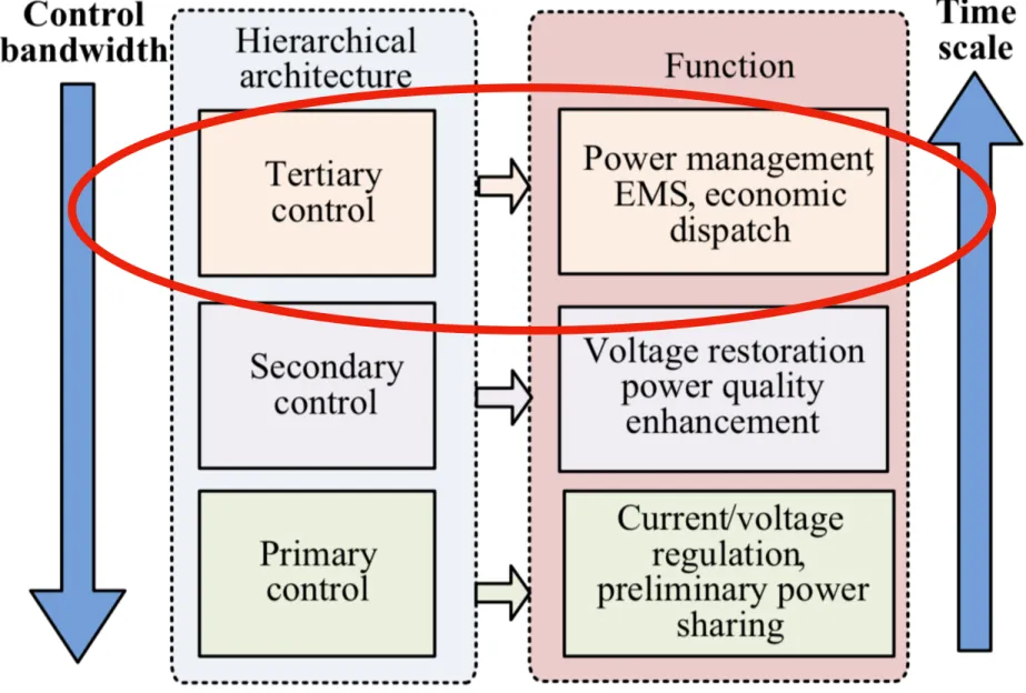
Fig. 1 Hierarchical control architecture.

Microgrid hierarchical control

Literature: two-layer approach Schedule layer:

-

-

Dispatch layer:

-

-

How interact the schedule and dispatch layers ?

Two-layer approach intensively studied:

[2] Jiang, Quanyuan, Meidong Xue, and Guangchao Geng. "Energy management of microgrid in grid-connected and stand-alone modes." IEEE transactions on power systems 28.3 (2013): 3380-3389.

[3] Wu, Xiong, Xiuli Wang, and Chong Qu. "A hierarchical framework for generation scheduling of microgrids." IEEE Transactions on Power Delivery 29.6 (2014): 2448-2457.

[4] Sachs, Julia, and Oliver Sawodny. "A two-stage model predictive control strategy for economic diesel-PV-battery island microgrid operation in rural areas." IEEE Transactions on Sustainable Energy 7.3 (2016): 903-913.

[5] Cominesi, Stefano Raimondi, et al. "A two-layer stochastic model predictive control scheme for microgrids." IEEE Transactions on Control Systems Technology 26.1 (2017): 1-13.

[6] Ju, Chengquan, et al. "A two-layer energy management system for microgrids with hybrid energy storage considering degradation costs."

PSCC 2020

Summary

1. Problem formulation

2. Proposed method

3. Case study description

4. Numerical results

5. Conclusions & perspectives

PSCC 2020

Abstract problem formulation

This problem is very difficult to solve since the evolution of the system is uncertain,

actions have long-term consequences, and are both discrete and continuous.

a⋆ 𝒯l(t) = arg min ∑ t′∈𝒯_l(t) c(a_t′, s_t′, ̂ω_t′) s.t. _{∀t′ ∈ 𝒯l(t), st′+Δt′ = f(at′, st′, ̂ωt′, Δt′),} s_t′ ∈ S′_t a_t = (am t , atd) s_t = (s_tm, s_td)

Actions set: market related (m) and set points to the devices (d).

Microgrid state: related to the market (m) and devices (d).

c f

Cost function.

Transition function of the system.

̂ω_t Uncertainty.

(1)

Summary

1. Problem formulation

2. Proposed method

3. Case study description

4. Numerical results

5. Conclusions & perspectives

PSCC 2020

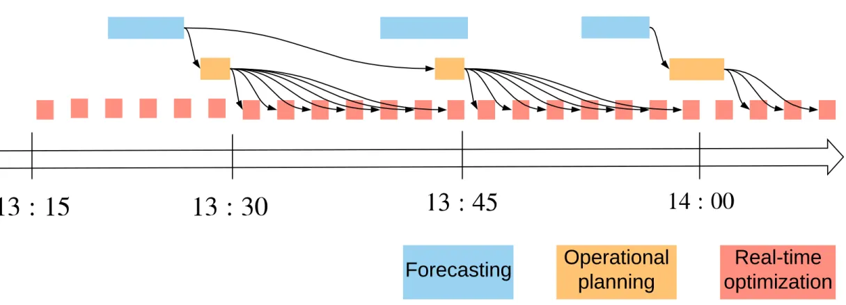
Forecasting Operational planning Real-time optimization Planner

PSCC 2020

Proposed method: two-layers with a value function

Fig. 2 Hierarchical control procedure illustration.

Two-layers approach with a value function to propagate information from

PSCC 2020

Proposed method: two-layers with a value function

am,⋆ 𝒯_ma(t) = arg min ∑ t′∈𝒯m a(t) cm_(am t′ , st′, ̂ωt′) s.t. ∀t′ ∈ 𝒯m_a(t), s_t′+Δτ = f m(a_t′m, s_t′, ̂ω_t′, Δτ) s_t′ ∈ S_t′ (2) Operational planner: Real-time controller: ad,⋆ t = arg min cd(atd, st, ̂ωt) + vτ(t)(sτ(t)) s.t. s_τ(t) = fd(a_td, s_t, ̂ω_t, τ(t) − t) s_τ(t) ∈ S_τ(t) (3) v_t(s_τ(t)) Value function at the end of the first market

PSCC 2020

Proposed method: objective function of the operational planner

COP t′ = ( ∑ d∈𝒟she Δ_τπshe d,t′Cd,t′shead,t′she + ∑ d∈𝒟ste Δ_τπste d,t′Cd,t′stead,t′ste + ∑ d∈𝒟nst Δ_τπnst d,t′Cd,t′nstad,t′nst + ∑ d∈𝒟sto

Δ_τγ_dsto_(Pdη_dchaa_d,t′cha + Pd

ηdis

d a

dis d,t′)

− πe

t′e_t′gri + πt′ii_t′gri₎ selling/purchasing energy to/from the grid

shed demand steered generation non steered generation

storage fee

DOP

t′ = πpδpt′ − πOPs r_t′sym peak cost and symmetric reserve

JOP

𝒯_ma(t) = ∑

t′∈𝒯m

a(t) (C

OP

t′ + Dt′OP₎ (4) Immediate and delayed costs.

PSCC 2020

Proposed method: objective function of the real-time controller

JRTO

t = CtRTO + DtRTO + vτ(t)(sτ(t)) (5) Immediate, delayed costs, _{and value function.}

Real-time controller:

Value function = cost-to-go at the end of the ongoing market period as a

function of the state of charge.

Evaluated by solving (4) for several states of charge = parametrization by

changing the RHS -> provide cuts.

Cut 1 to 3: s_τ(t) = s₁ [μ₁] → v_τ(t)(s) ≥ v_τ(t)(s₁) + μ₁Ts s_τ(t) = s₂ [μ₂] → v_τ(t)(s) ≥ v_τ(t)(s₂) + μT 2 s s_τ(t) = s₃ [μ₃] → v_τ(t)(s) ≥ v_τ(t)(s₃) + μT 3 s

Summary

1. Problem formulation

2. Proposed method

3. Case study description

4. Numerical results

5. Conclusions & perspectives

PSCC 2020

MiRIS case study

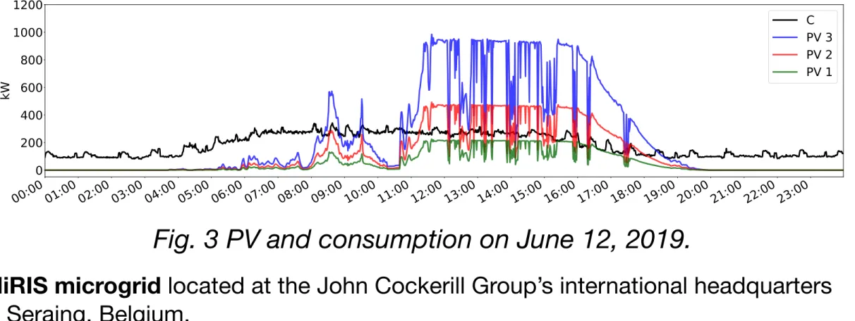
Fig. 3 PV and consumption on June 12, 2019.

27 days of data (measurements and point forecasts) available on the Kaggle platform:

https://www.kaggle.com/jonathandumas/liege-microgrid-open-data

MiRIS microgrid located at the John Cockerill Group’s international headquarters

in Seraing, Belgium.

https://johncockerill.com/fr/energy-2/stockage-denergie/

PSCC 2020

MiRIS case study: managing the peak penalty

Table I: Case study parameters.

C = load S = Battery

Peak penalty if import > 150 kW paid at 40 euros / kW Day/night import prices: 200/120 euros MWh.

Single export price 35 euros /MWh.

Summary

1. Problem formulation

2. Proposed method

3. Case study description

4. Numerical results

5. Conclusions & perspectives

PSCC 2020

Numerical results: RTO-OP vs RBC

Planner (OP):

-

-

-

Controller (RTO):

-

-

PSCC 2020

RTO-OP is compared to a Rule Based Controller (RBC).

Numerical results: RTO-OP vs RBC

PSCC 2020

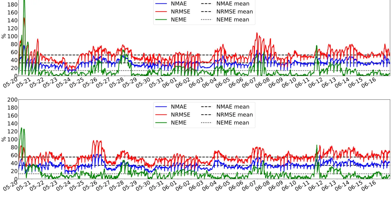
PV and consumption weather based point forecasts for OP use

Recurrent Neural Network (RNN) and Gradient Boosting Regression (GBR) techniques.

The weather forecasts provided by the Laboratory of Climatology of the

Numerical results: peak management

PSCC 2020

Table II: Results without symmetric reserve.

energy cost (k euros) peak cost (k euros) total cost (k euros) peak power (kW)

RTO-OP is still a long way to manage the

peak as RTO-OP* due to the forecasting errors.

RTO-OP optimizes PV-storage usage, and

thus requires less installed PV capacity for

a given demand level than RBC.

c_E c_p

c_t = c_E + c_p Δ_p

PSCC 2020

RTO-OP tends to maintain a storage level that allows to better cope with forecast error.

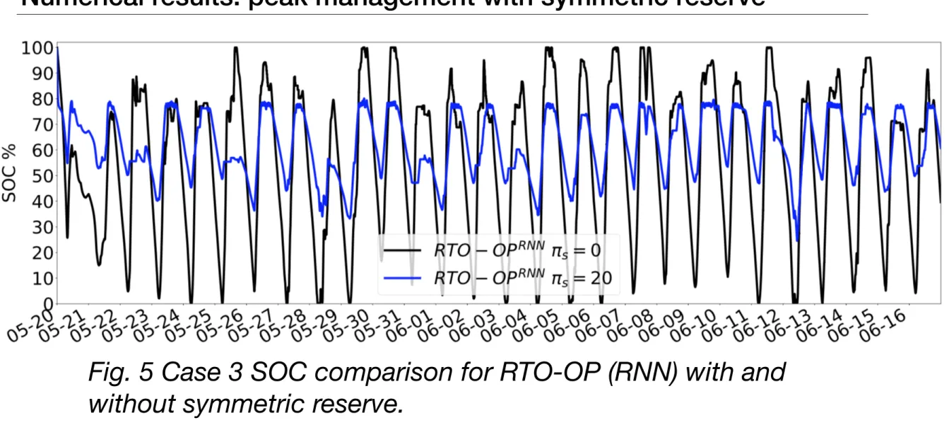
Numerical results: peak management with symmetric reserve

Fig. 5 Case 3 SOC comparison for RTO-OP (RNN) with and without symmetric reserve.

PSCC 2020

Table III: Results with symmetric reserve for RTO-OP (RNN)

There is an economic trade-off to reach to manage the peak and the

reserve simultaneously depending on the valorization or not on the market of the symmetric reserve.

The peak power has decreased. Numerical results: peak management with symmetric reserve

Summary

1. Problem formulation

2. Proposed method

3. Case study description

4. Numerical results

5. Conclusions & perspectives

PSCC 2020

Conclusions & extensions

The value function computed by the operational planner based on PV

and consumption forecasts allows to cope with the forecasting

uncertainties.

The approach is tested in the MiRIS microgrid case study with PV and

consumption data monitored on site.

The results demonstrate the efficiency of this method to manage the

peak in comparison with a Rule Based Controller.

Extension to a stochastic/robust formulation to deal with

probabilistic forecasts.

Extension to a community by considering several entities inside the microgrid.

Annex: Point forecasting methodology Inputs:

-

-

Outputs:

- PV production / load 24 ahead hours with 15 min resolution

The point forecasts are computed on a quarterly basis using a Long Short

Term Memory (LSTM) with the keras python library [8] and a Gradient Boosting Regression (GBR) with the scikit-learn python library [9].

The forecasting process is implemented using a rolling forecast

methodology. The Learning Set (LS) is refreshed every six hours and

limited to the week preceding the forecasts.

[8] F. Chollet et al., “Keras,” https://keras.io, 2015.

Annex: Point forecasting results

PSCC 2020