The Prediction of Fund Failure through Performance Diagnostics
* This version: June 15, 2014Philippe Cogneaua Georges Hübnerb
Abstract
Using an international database featuring 1,624 mutual funds over 15 years, this paper analyses the joint abilities of performance measures to predict subsequent fund failure. We examine the probability of disappearance over a time window, and expected fund survival time, and study the circumstances of a fund’s disappearance, its currency and domicile. By combining relevant measures, fund failure appears to a significant extent predictable, more than with single classical
* We thank Régis Houyoux, Julien Vandenborre, Atanas Djondjourov and Stéphanie Delhalle for valuable research
assistance, and Fernando Tenorio for his technical help. We also express our gratitude to an anonymous referee,
Laurent Bodson, Nicolas Callens, Serge Darolles, Georges Gallais-Hamonno, Alain Jousten, Bernard Lalière, Marie
Lambert, Pierre-Armand Michel, Bertrand Maillet, Xavier Mouchette, Maud Reinalter, and the participants of the
2011 Workshop on Investment Funds (Luxembourg), the 2012 Congress “Forecasting Financial Markets”
(Marseille) and the Seminar “Finance and Economic Development” (El Jadida) for helpful comments. All errors are
our own.
aAssociate Researcher, HEC - Management School of the University of Liège, Belgium; Lecturer, EDHEC, Lille,
France; Lecturer: Haute Ecole Fr. Ferrer, Brussels, Belgium;. E-mail: [email protected]
bCorresponding author. Deloitte Chair of Portfolio Management and Performance, HEC - Management School of the
University of Liège, Belgium; Associate Professor of Finance, School of Business and Economics, Maastricht
University, Maastricht, The Netherlands; Chief Scientific Officer, Gambit Financial Solutions, Belgium; and
Affiliate Professor of Finance, EDHEC, France. Tel. (+32) 4 2327428. Fax (+32) 4 2327240. Address: HEC-ULg,
measures. Survivorship predictability has significant economic value. Such evidence suggests that past performance does not only influence investors’ perception of fund quality, but also reflects managers’ ability to sustain performance.
Keywords: Fund survival, performance measurement, persistence analysis, mutual funds JEL classification: G10; G11; G14; G17
1.Introduction
For different reasons, mutual fund survivorship has been an ongoing concern since the early 1990s. Many researchers have studied this phenomenon because of the so-called “survivorship bias”. Ignoring funds that disappear while analyzing their performance generates an important bias: since the funds that failed during the period are omitted, only the funds that stayed alive during the whole period are selected. Another collection of papers has focused on the assessment of the percentage of “graveyard” funds, i.e. those that disappear within a certain period. But only few studies have aimed to examine the determinants of fund terminations. Even though the field of performance measurement has considerably expanded since the turn of the century, no recent paper has related funds disappearance to an extensive review of their past risk-adjusted performance beyond the classical measures developed in the sixties and seventies.
A first stream of papers relates a fund’s fate to its past returns. Through their analysis of the determinants of mutual funds survivorship, Brown and Goetzmann (1995) uncover the link between the likelihood of fund disappearance with its past returns, going back three years. Carhart (1997) even finds that dead funds underperform until five years before their disappearance. Brown et al. (1997), Malkiel (1995) and Elton et al. (1996) show that only the best performers survive for a long period of time, while weaker ones are likely to be closed. Cameron and Hall (2003) discover that excess returns relative to a market index are much better predictors of fund failure than gross returns. They obtain an asymmetric link between shocks and disappearance: positive shocks have a larger impact than negative shocks.
In parallel, some researchers have focused on the reasons underlying fund terminations. Sawicki (2001) and Sirri and Tufano (1998) point out that investors base their fund purchase decisions on prior performance. However, in most studies following this approach, the authors solely focus on classical performance measures: gross return, return on excess of a market index,
Jensen alpha (Jensen, 1968), Fama and French 3-factors alpha (Fama and French, 1993), Carhart 4-factors alpha (Carhart, 1997). Rohleder et al. (2011) compare the results given by the last four different measures to estimate the size of the survivorship bias obtained with different methods with US mutual fund data.
Recent research on mutual fund survival has largely diverged from the examination of past performance as a predictor of failure. Many other determinants of fund death have been investigated: size (Brown and Goetzmann, 1995; Carhart et al., 2002), age (Brown and Goetzmann, 1995; Lunde et al., 1999), style (Horst et al., 2001; Bu and Lacey, 2009), expense ratios (Carhart et al., 2002; Bu and Lacey, 2009) or incentives (Massa and Patgiri, 2009), among others. The interest in prior performance and risk as predictors of fund failure has migrated to the hedge funds literature. In their analysis, Liang and Park (2010) consider different risk measures to adjust performance. They show that semi-deviation, value-at-risk, conditional value-at-risk, expected shortfall and tail risk are better predictors than standard deviation (especially the latter two).
Other studies, such as Chapman et al. (2008) and Ng (2008), develop models aiming at forecasting hedge fund failure. They use the same performance metrics mentioned in the literature devoted to mutual fund analysis. Darolles et al. (2014) focus on the dependence in the liquidation risk. They consider two aspects: exogenous stochastic factors that can have a mutual influence in the liquidation intensities of the individual funds, and are often called frailties (Duffie et al., 2009). They can explain the high likelihood to observe a high percentage of default at a given date. On the other hand, a contagion effect appears when an event on a fund has an impact on other funds – for instance funds invested in other funds. It can be an answer to time series dependence on fund failure: high intensity in the closing during a given period followed by a high intensity during the next period.
In this paper, we refer to the intuition that past performance would naturally stand as a primary determinant of the decision to shut down a mutual fund. At the same time, we acknowledge that the literature on performance measurement has considerably evolved since the seminal studies in the field, and wish to take advantage of this progress. Our study aims to systematically investigate the drivers of past performance and to detect whether a multi-dimensional representation of a fund’s performance reveals helpful in predicting its survival. We make full use of the spectrum of performance measures rather than sticking to the most classical and/or popular ones. By doing so, we investigate a specific research hypothesis: do the reasons for shutting down a fund go beyond the mere perception of past performance by investors – which would be the case if only a few set of measures sufficed to explain fund failure – or are they more likely related to the intrinsic qualities of the fund manager, as represented by a more sophisticated and multi-dimensional array of performance metrics?
To the best of our knowledge, ours is the first paper dedicated to the comprehensive analysis of the predictive properties of performance measures for fund survival. Our focus on forecasting the probability of survivorship rather than on persistence in performance is motivated by a hierarchical concern. For an investor, it is much more important to be able to anticipate a fund’s death than to be able to pick superior future performers, because the consequences of making the wrong bet are far more penalizing in the first case. Consistent with this objective, we concentrate our analysis on the detection of the best predictive association of performance measures as a whole, rather than on the economic and statistical significance of each individual predictor. For the same reason, we develop and test our model with non-overlapping time windows. This leads us to consider its in-sample fitting quality as well as its out-of-sample predictive capacity.
Our comprehensive analysis also introduces three improvements over previous studies, namely the use of weekly data, the coverage of different international fund markets1, and the consideration of dependence between liquidation times. Finally, we also distinguish the reason for a fund’s disappearance and examine the predictability in specific market segments and conditions.
The paper is organized as follows: Section 2 presents the data and the construction of variables. In Section 3, we analyze the link between a fund’s past performance and its probability of disappearance. Section 4 presents the concluding remarks.
2.Data and variable construction 2.1. Mutual fund and market data 2.1.1. Mutual fund data
We exploit a database of weekly2 returns for 2,794 open-ended accumulation3 mutual funds with major or full allocation in equities on a worldwide basis. The time window ranges from Friday
1 Most of the research focuses on US data or other national markets (e.g. Australia in Cameron and Hall (2003) and
Sawicki (2001), and the United Kingdom in Lunde et al. (1999)).
2 The choice of weekly data represents a compromise between the superior ability to detect market timing effects
with higher frequency data (“Our results motivate the use of daily data in future tests of mutual fund performance“,
Bollen and Busse, 2001) and evidence of higher potential bias due to benchmark misspecification with the use of
daily fund returns (Coles et al., 2006). In parallel, we face a problem of operational efficiency. Many measures are
regression-based, preventing the use of monthly data for short time windows. On the other hand, weekly data permits
a quicker and therefore more precise detection of the delisting, inducing better precision when building the logistic
December 30th 1994 to Friday January 8th 2010, so 15 years of returns. We extend the sample to July 2011 in order to gather observations of each fund’s survival or attrition posterior to the data period. Returns are extracted from Thomson Reuters Datastream4.
The database is further contaminated with a number of potential sources of interferences. To mitigate their effects, we apply the following filters: (i) we exclude from the sample all funds for which the missing data or variability in the series of weekly prices are potentially suspicious. All funds having missing data in their price series, at least three times three consecutive identical prices, or at least eight times two consecutive identical prices, are rejected; (ii) if the shares of a fund have once been divided or regrouped, we recalculate the whole series of prices starting from the day of the event, to ensure coherency in the series; (iii) we perform a global check of the plausibility of the prices: in particular, for a dozen of cases, a manual research has been done to fix some prices in the series; (iv) we eliminate 140 “cousin” funds, by regressing the returns of funds suspected to be similar, and excluding one of them when the correlation is higher than 80%; (v) a return-based style analysis enables us to eliminate some funds invested in bonds or in short-term fixed income securities; and (vi) to obtain homogeneity in the asset pricing specifications used to compute multiple performance measures, we keep only the funds denominated in the five most important currencies (i.e. GBP, EUR, USD, CHF and JPY).
3 The type of the fund is cross-checked through a manual research in Bloomberg. We avoid the issue of the
distribution of dividends, which may have a tax impact for investors in different countries, by restricting the sample
to only open-ended accumulation funds without stated initial maturity.
4 Because of the international character of the study, we preferred relying on a single database instead of mixing
non-US data from Thomson Reuters Datastream with the survivorship bias-free CRSP Mutual Fund database.
Nevertheless, we manually ran a number of probes to ensure the consistency of data retrieved from Thomson Reuters
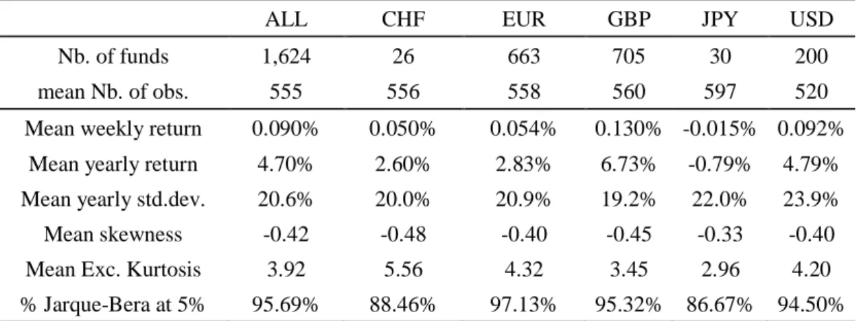
This leaves us with a final sample of 1,624 funds: 705 in GBP, 663 in EUR, 200 in USD, 30 in JPY and 26 in CHF5. Considering the country of domiciliation, we get 695 funds issued from the United Kingdom, 405 from Luxembourg, 178 from France, 114 from Italy, 89 from Belgium and 58 from Austria6. Other countries (Switzerland, Germany, Ireland, Liechtenstein, USA and Virgin Islands) are present in less than 50 funds. Summary statistics about these 1,624 funds are given in Table 1.
[ Insert Table 1 approximately here ]
Even though the sample period encompasses the 2007-08 crisis, average yearly returns are positive. They are higher for funds denominated in GBP or issued in the United Kingdom, but lower for Austrian and even negative in JPY. Standard deviations are in the neighborhood of 20% for all currencies. Skewness is always negative, and kurtosis is very positive.
The last row indicates the frequency at which the hypothesis of normally distributed returns can be rejected at the 5% confidence level using the Jarque-Bera statistic. More than 95% of the funds exhibit a pattern leading to the rejection of the null. Thus, performance measures solely based on the mean-variance framework are likely to produce inaccurate outputs for most funds. The use of a larger array of performance measures for these funds is warranted.
5 The condition on accumulation excludes a large number of funds denominated in USD, which explains their lower
presence, but the sample size remains sufficient to draw statistical inferences.
6 We are aware that a fund’s administrative domicile does not necessarily indicate that the fund is managed in the
same country. For instance, Luxembourg is renowned for being a popular place for fund administration, but few
managers are headquartered in this country. Nevertheless, the country of a fund’s administration is still important
information regarding its propensity to survive, as the legal, tax, and service environment can also bring significant
The database reports 978 live funds at the end of the pricing period, which even shrinks to only 856 (52.7%) if we consider a snapshot 18 months later. For the 769 defunct funds, we make a manual search on Bloomberg or with internet sources to retrieve the reason for delisting. We distinguish the following reasons for a fund ceasing to report returns7: (a) the fund has merged by absorption with another fund; (b) the fund has been liquidated; (c) the fund has become inactive for another reason; (d) the fund is still alive but has been delisted from the database.
Table 2 partitions delisted funds by year, currency, country and delisting type. [ Insert Table 2 approximately here ]
The percentage of graveyard funds is higher for those denominated in GBP and USD, and incorporated in the UK and Luxembourg. It is much lower for Belgian and Italian funds.
The main two reasons for disappearance of a fund are its merger with another fund and its liquidation. We also find evidence of more mergers for GBP and USD funds, or issued in the UK and Luxembourg. There are proportionally more liquidations in Austria and Luxembourg.
Very few funds disappeared before 2002. Markets were very bullish (dot-com bubble) until 2000, and few funds die when their returns are positive even with a disappointing performance. 2.1.2. Market data
To determine the risk-free rate, we consider the 3 months Treasury Bill in the currency of the fund. When it is available, we use the main stock index of the country where a fund was issued, as proxy for the market. In the case of small countries, like Liechtenstein, we take the index of the most important neighbor country – or the average of the neighbor countries, in the case of
7 In most cases, we find the exact delisting date of the fund. If such information is not available from our multiple
sources, we consider the last reported price date as the one of disappearance. Considering all funds for which we get
the information, the difference in days between the last price and the disappearance is lower than 7 days in the
Luxembourg. Inflation rates8 of the involved countries are retrieved from various official sources of information, mainly Central Banks and Eurostat.
Some performance measures, like the Information ratio, the Generalized Black-Treynor ratio or the Total risk alpha, either require the specification of a return generating process or the identification of a benchmark portfolio for the fund under review. We adopt the return-based style analysis framework proposed by Sharpe (1992). There are two reasons for this choice. First, this approach leads to superior benchmark definition over self-reported benchmarks for many funds. Second, we can define a benchmark for all funds, including absolute or total return funds, which is necessary in order to produce a large number of performance measures.
We select 41 indexes9 representative of most of the world markets. A part of them is geographical delimited, including North American, European, Asian, and emerging markets; we also consider index restrained to small or mid or large capitalizations. The remaining ones are sector indexes, gold and oil. To determine the benchmark of each fund, we then apply the strong form style analysis (Sharpe, 1992), considering the 41 index returns converted in the fund’s home currency, and a 42nd index which is the risk free rate in the same currency. The selection of style indexes for each fund is refined using the procedure described by Lobosco and DiBartolomeo (1997). We implement it by the following process:
- As a first step, we regress the returns of the fund on the 42 potential benchmarks, to determine 42 positive weights. We compute the standard deviation of those weights and set the 95% confidence interval for each weight. From this first step, we retain all indexes having a strictly positive weight and an upper bound greater than 10%.
8
Inflation rates present strong seasonal variations, so we compute systematically the yearly mobile average.
9
- We reiterate the procedure with the selected set of indexes. For all further steps, we keep all potential benchmarks having a strictly positive weight and an upper bound greater than 20%. - We stop the process when no index exits from the list or when there remain only two indexes
– one of them being the risk free one. 2.2. Computation of performance measures
Cogneau and Hübner (2009 and 2009a) report more than one hundred portfolio performance measures developed in the academic and practitioner’s literature. We select about 70 of those measures and compute them on the sample of funds. For parametric measures, we consider multiple variations. For instance, we often consider three variants when a reference return is needed: risk-free rate, inflation rate, zero percent; we compute measures using the Value-at-Risk or the Conditional Value-at-Risk with different thresholds; different values of the parameters are used to reflect the price of the risk or the investor’s style, in measures like Farinelli-Tibiletti ratio, Sharpe’s alpha or Aftalion and Poncet’s index10. This leads us to the computation of 147 performance measures, whose detailed list can be found in the Appendix11.
We compute the linear returns and then the 147 measures over various time scales (annual, from one to five years), considering moving windows rolling every week over the full sample period. This yields a maximum of 14 x 52 x 147 = 107,016 individual one-year performance estimates for a fund with full history. We finalize this step of computation by centering and
10 The complete parameterization of these variations and the source documents are available upon request.
11 The computation of alphas with conditional models require lagged values of some macroeconomic variables; as
Christopherson et al. (1999), we retain the yield spread (spread between the 10 years and the 3 months interest rates)
and the credit spread (spread between BAA and AAA rated corporate bonds); as third variable, we considered the
inflation rate (see Chen et al. 1986; Ferson and Harvey, 1995); finally, we add the volatility (Bollerslev et al., 2011)
standardizing each measure, to get their normalized versions. These values will be used in the forthcoming analysis.
2.3. Selection and processing of relevant performance measures
To eliminate the redundancies showing up in the series of 147 of computed performance estimates, we proceed as follows. For each year, we compute the matrix of Kendall’s rank correlations between the 147 measures. Then, we build an average of the 15 yearly matrices, and remove all collinear measures with a stepwise elimination procedure. The set of remaining measures have two-by-two correlations that do not exceed 85%12. About two thirds of the measures are rejected. Table 3 summarizes the classes of the 56 remaining measures.
[ Insert Table 3 approximately here ]
The main distinctive aspects of performance emphasized in the taxonomy presented in Cogneau and Hübner (2009 and 2009a) show up in the results: market timing (alphas and gammas of Treynor-Mazuy and Henriksson-Merton); preference-based (prospect ratio, Stutzer index); return-based ratios (Sharpe ratios based on VaR and CVaR, variations of Sortino and Information ratios, Generalized Black-Treynor ratio…); gain-based ratios (Farinelli-Tibiletti ratio, Rachev ratio…); return-based differences (M2 and various alphas: Jensen, Fama & French, total risk); and gain-based differences (Fouse index). The control for systematic risk is clearly distinguished from the non-systematic one, as we retain both the Modified Jensen and Moses, Cheney & Veit’s measures.
When a variation of a measure takes skewness and kurtosis into account, it is often selected. As a consequence, some of the most classical measures, as Sharpe ratio, Treynor ratio, Sortino
12 We also process computations with thresholds of 80% and 90%, with no significant difference in the results
ratio, are discarded in their original form. Enhanced measures seem thus to be more appropriate in the framework of a predictive analysis.
With the 56 potential measures, we define dummy variables corresponding to the quintiles of the selected measures. This treatment enables us to perform quintile regression. Koenker and Hallock (2001) show that quintile variables allow considering different effects along the distribution of the dependent variables. This enables to match a non-homogeneous relation with the independent variable (saturation effect, S-shaped curve…). Quintile regression is also more robust to outliers.13
2.4. Introduction of contagion and frailty variables
The methodology described in next section assumes implicitly the independence of individual delisting times. However, we check the uniformity over time of the delisting distributions through a Kolmogorov-Smirnov test, and the uniformity is rejected at the 95% threshold. This leads us to complement the performance measures with additional independent variables that could adequately proxy for the time-clustering of attrition events.
In the context of hedge funds, Darolles et al. (2014) explore the dependence in the liquidation risk and emphasize two causes of liquidation risk dependencies. On the one hand, the high likelihood of observing a high percentage of delistings during a given period can find its origin in underlying exogenous factors having a common influence on the liquidation risks of the individual funds. They call these factors frailties. On the other hand, a high percentage of funds attrition during a certain time interval immediately followed by a high proportion of subsequent
13 We have also used the performance measures themselves, but the results appear to be less significant both in- and
delistings can be explained by a contagion phenomenon: a shock to one fund has an impact on the other funds that belong to the same class.
To represent these phenomena within our modelling approach, we introduce two series of variables, measured at a given time t. The first one is the percentage of funds in the whole sample that closed during the lagged period [t-τ,t[. This variable proxies for the frailty effect. The second one is the percentage of funds that closed during the last period in a given class, defined as the group of funds that share the same primary index in the constitution of their benchmark (see section 2.1). This second variable stands for the contagion effect. Regarding the duration of the lagged period covered by these two variables, we consider the three following lengths τ: one week, one month (4 weeks), and one quarter (13 weeks).
3. The link between fund performance and subsequent disappearance
We apply our approach on the global sample of funds. Next, we study the past performance as determinant of the predictability of fund disappearance, by type of fund death, country of incorporation, currency of denomination and by market trend.
3.1. Methodology
To analyze the potential link between the performance of a fund and its disappearance, we execute a logistic regression, where the independent variables are the frailty and contagion variables defined in subsection 2.4, the quintile variables corresponding to the selected 56 normalized measures, and the dependent variable is a dummy representing the disappearance of the fund: 1 = ( , + , ′ Π , ;) 1 + ( , + ′, Π , ;) (1)
where τi is the time of disappearance of fund i, T is the length of the prediction period, in years (T = 0.25, 0.5, 0.75, 1 or 1.5), h is the horizon for prior performance measurement, in years (h = 1, 2, 3, 4 or 5), Π , ; is the vector of quintile dummies for the selected performance measures, and
αh,T and B’h,T are the estimated coefficients of the regression.
To check the significance of the results, we consider Somers’ D14 as a synthetic indicator of the ability of the performance measures to predict the disappearance time of the fund (Somers, 1962). This statistic has a geometric interpretation15 similar to the Gini coefficient in the context of the logistic regression: if we divide it by 2 and we add 0.5, we obtain Harrell’s c statistic, which is the area below the Receiver Operating Characteristic (ROC) curve.
We build the model of the logistic regression with a stepwise algorithm with forward variable selection (see e.g. Butera and Faff (2006), Hu and Ansell (2007), Niklis et al. (2012)). We start by ranking Somers’ D for each measure considered individually in a logistic regression. We build a first model with only one measure – the one with the highest individual Somers’ D –
14
This indicator, computed on the binary outcome, is intensively used in credit risk (see for instance Laitinen (1999)
or Melnik and Plaut (1996)) to quantify the capacity of the estimated risk score in discriminating the defaulting
versus the non-defaulting entities. An alternative is the Hosmer-Lemeshow goodness-of-fit test. However, this test is
not usable with our large database as Paul et al. (2013) have reported that in very large data sets (n > 25,000), small
departures from the proposed model will be considered significant.
15 Somers’s D is computed as follows: S = (C – D) /(C + D + T) where C is the number of concordant pairs, D is the
number of discordant pairs and T is the number of tied pairs (pairs of observations that have equal values of
observations or equal values of predictions). A pair of observations with different observed responses is said to be
concordant if the observation with the lower ordered response value has a lower predicted mean score than the
observation with the higher ordered response value. If the observation with the lower ordered response value has a
higher predicted mean score than the observation with the higher ordered response value, then the pair is discordant.
and compute the Schwarz Criterion (SC) of this model. Then, we loop on the 55 remaining measures, by decreasing16 individual Somers’ D. At each step, a new measure is added in the model and a new logistic regression is executed. If the Schwarz Criterion increases, the variable is rejected. If the Schwarz criterion decreases but the weight of the measure is not significant enough (level set at 20%), we check the evolution of the Somers’ D: if it does not increase, the variable is also rejected.
We ensure the robustness of our model by cutting the sample in two sub-samples of similar sizes: one for the training of the model (“modeling group”), the second as a validation group. The algorithm that builds the two subsamples guarantees that the number of records for each currency and each country are about the same17. In order to avoid contagion in the data when applying the model on the validation group, we ensure that all instances of a fund are present in the same subsample.
To avoid a bias in the comparison of models with different length in the performance period, we consider the same periods for the predictions, starting from January 2000. It means that the first performance periods start in 1999 for one-year performance, and in 1995 when performance is measured over five years. As a second step, the same process is re-executed, starting with first models that include not only one measure but also the frailty and contagion variable as defined in subsection 2.4.
16
For the first four iterations, we add a condition on the selected measure: its correlation with the measures already
in the model must be under a predefined threshold – this is to ensure a sufficient variety of the selected measures.
17 Detailed statistics of the number of funds in the modeling and validation groups, by duration of observation period,
3.2. Global results
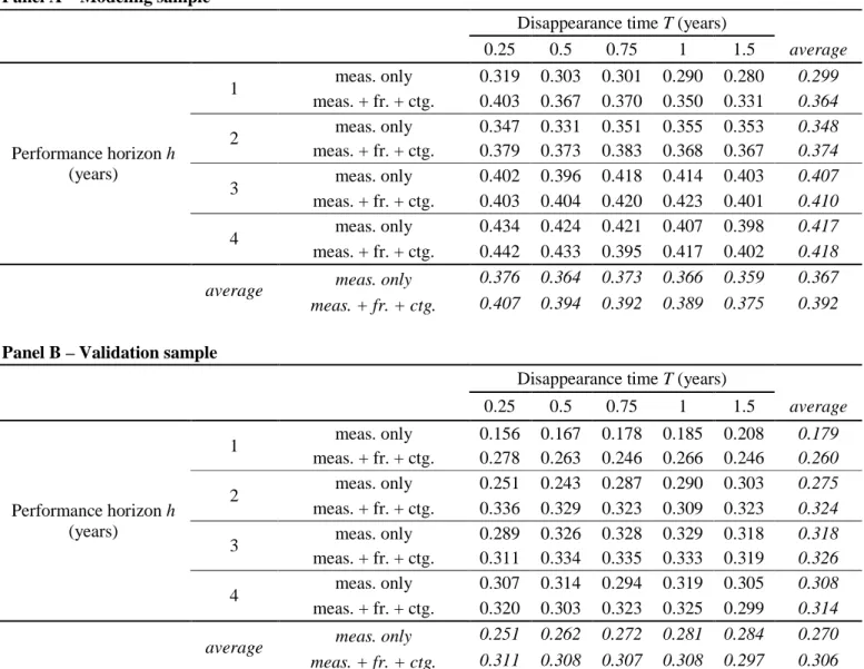
Our results on the global sample18 are summarized in Table 4.
[ Insert Table 4 approximately here ]
The values displayed in Table 4 suggest that the disappearance of a fund is largely predictable according to its past performance19. In general, the longer the observed period, the better the prediction becomes. This tendency can be explained by the condition on survivorship over the performance measurement horizon: by restricting the sample of eligible funds to the ones that had been existing for a longer period, their likelihood of surviving longer is reinforced.
Up to four years are enough to get a good picture of past performance in the modeling group20. If we consider the validation sample, an observation period of three years is optimal. This is consistent with the finding of Lunde et al. (1999) that the performance over the previous three years matters more for a fund’s closure probability than its performance over the past year.
The introduction of the contagion and frailty variables computed over the previous quarter21 strongly improves the model for short durations of the performance period. Beyond three years however, the added value of the frailty and contagion variables becomes marginal: it is largely subsumed by the performance measures for three years or more, which appear to capture the
18 We also process the same computations considering subsets of the whole sample, keeping only one period on four
(monthly starts) or one period on thirteen (quarterly starts). The results remain essentially unaltered.
19 We compute the confidence interval for the Somers’s D, using the method of Newson (2006): due to the large
number of records in the sample, the size of the confidence interval at 95% is almost always less than 0.005. The
values indicated in Table 4 and the subsequent ones are therefore highly significant.
20 Increasing the measurement horizon to 5 years leads to a reduction of the model accuracy for both sub-samples. 21 The explanatory power of the same variables on shorter durations (one week or one month) is smaller (results not
dependencies between individual liquidation times. In other words, the funds’ past performance over long horizons seems to act as a predictor of their tendency to disappear by clusters, and so the frailty and contagion variables become largely redundant.
Regarding the duration of the disappearance prediction period, no clear trend emerges. The quality of the prediction is almost the same, whether the observation period is three months or higher. More precisely, without the inclusion of the contagion and frailty variables, it decreases slowly with the length of the prediction period in the modeling sample, and it increases at a similar rate in the validation sample. As the influence of contagion and frailty is more pronounced for shorter periods, the predictability of models including these effects decreases as the duration increases.
Panel C of Table 4 reports that on average, slightly less than one half of the potential measures are kept in the final specification. This number increases with the duration of the disappearance period. Reported results confirm the higher predictive power of contagion and frailty for shorter durations.
In Table 5, looking more closely into the parameter estimates for the retained measures in the best case for the validation sample (i.e. performance horizon h is 3 years, disappearance period T
is 12 months), return-based measures have the most important weight22 in the predictive power of the model. Conversely, market timing measures reflect a negative persistence.23
[ Insert Table 5 approximately here ]
Considering the frailty and contagion variables, the positive sign of the coefficient for the contagion and the negative sign for the frailty leads us to the conclusion that contagion effects, which reflect a more concentrated clustering effect, have a more important impact than frailties.
Figure 1 displays the ROC curves for the modeling sample and for the validation sample, in the same case (h = 3, T = 1, inclusion of contagion and frailty variables). The diagonal corresponds to the random pick. The graph provides a visual correspondence of the values taken by Somers’ D of 0.423 and 0.333 provided in Table 4, which corresponds to the values 0.712 and 0.667 for Harrell’s c. The area under the ROC curve for the modeling sample amounts to more than 70% of the total size of the box. We also emphasize the smoothness of this curve, which indicates that the quality of the prediction remains stable throughout the sample. The value of the logistic function depicted in equation (1) is almost proportional to the probability of disappearance.
[ Insert Figure 1 approximately here ]
22 As the target value of the logistic regression is +1 for the delisted funds, a negative coefficient for a measure
means that it has a good positive predictive power.
23
We consider further the differences of measures (relative and absolute change) as potential independent variables.
It is well documented in the domain of credit risk modeling, which is relatively close to ours, that the inclusion of
differences in parameters often gives better results. This extension is justified by the conjecture of a similar effect
appearing here. Even though the inclusion of absolute and relative difference in performance measures increase the
Somers’ D in the modeling sample, the results become generally poorer in the validation sample for horizons longer
3.3. Specific aspects of predictability
3.3.1. Prediction by reason for disappearance
Three potential reasons are reported for the disappearance of a fund: “liquidation”, “merger”, “inactivity”, and funds for which no justification are given being classified as “other”. The latter two categories being very marginal, we group them with the first one for further analysis.
We first examine whether predictability is more or less pronounced according to whether delisting is due to liquidation or another form of fund freeze. While the first category of events eventually corresponds to fund death, the merger case entails that the money still remains invested in the fund, but through an absorbing vehicle. It is interesting to study to what extent past performance explains the distinction among survivors between live and absorbed funds.
[ Insert Table 6 approximately here ]
The predictable character of fund disappearance already observed in Table 4 is confirmed in panel A of Table 6. Partitioning the sample increases predictability, especially for mergers. For instance, the quality of the prediction (represented by Harrell’s c) of a merger when performance is measured over a 3-year horizon exceeds 75% for time windows of 12 months.
Not only the predictability of liquidation vs. merger differs, but we also note that different dimensions of performance influence the forecasts. Panel B of Table 6 compares the predictive power of the different classes of measures. Preference-based measures are highly predictive for mergers, while their forecasting power is smaller in the liquidation case. Conversely, the predictive power of market timing gammas is higher for liquidation than for mergers.
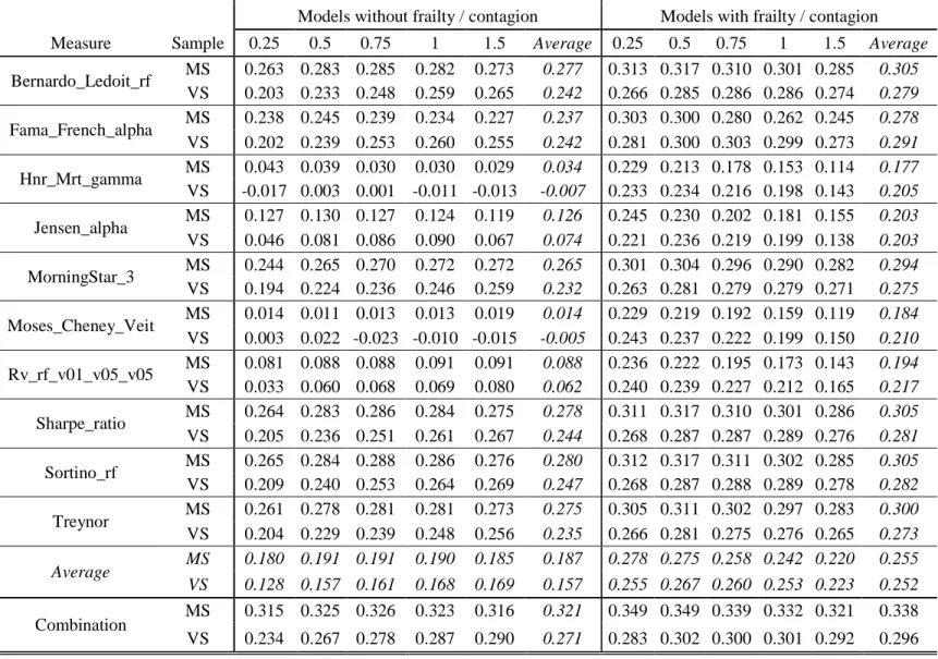
3.3.2. Predictability for classical measures
The use of such a large number of classical performance measures opens up the way to two types of biases: the possibility of data mining and the excessive importance given to irrelevant performance measures. To mitigate them, we restrict the sample to a limited subset of measures
whose selection is based on a qualitative assessment of their relevance and/or their popularity. For this purpose, we adopt 10 measures. By alphabetical order, these are: Bernardo-Ledoit ratio (aka Omega), Fama & French alpha, Henriksson-Merton gamma, Jensen’s alpha, MorningStar (risk coefficient of 3), Moses Cheney & Veit’s measure, Rachev ratio (parameters equal 0.05 and 0.05), Sharpe ratio, Sortino ratio (risk-free rate as reserve return), and Treynor ratio.
We first perform a logistic regression with each of these measures individually, computed on a period h of 3 years, as independent variable, and the disappearance (all five durations T, as in Table 3) of the fund as dependent variable. In a second step, we combine these 10 measures in a logistic regression where they are all considered as independent variables. The results are reported in the left side of Table 7.
[ Insert Table 7 approximately here ]
Compared with the value for Somers’ D obtained in Table 4, some measures provide reasonable predictability: the Bernardo-Ledoit ratio, Fama & French alpha, MorningStar, Sharpe ratio, Sortino ratio and Treynor ratio, often obtain a D estimate exceeding 0.25. It is noteworthy that a very popular regression intercept, Jensen’s alpha, is powerless, even though some other measures based on the same one-factor specification, like the Treynor ratio, are relevant. Taken altogether, the D index increases to values above 0.3, which are however lower than those obtained with the full set of measures (see Table 4). For instance, when the forecasting horizon is 6 months, the loss in accuracy in predictability amounts to (0.414 – 0.323)/2 = 4.5% for the modeling sample and to (0.329 – 0.287)/2 = 2.1% for the validation sample.
The right side of Table 7 reports the results for the same measures, but including the frailty and the contagion variables in the models. Compared to the reported results of Table 4, the Somers’ D are substantially higher even for the model that combines all classical measures. This
indicates that altogether, the classical measures taken individually are unable to capture the dependencies between individual liquidation times.
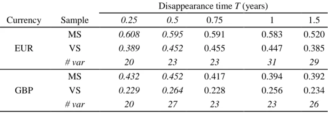
3.3.3. Predictability for subsets of funds
Finally, we examine whether the forecasting power of the logistic regression differs for different types of funds. We analyze two dimensions. The first one is the currency of denomination, and the second one is the country of domiciliation. We restrict the presentation of results in Table 8 to a horizon of three years for the performance measurement, to models including the contagion and frailty variables, to currencies EUR and GBP, and to countries UK and LU – which represent more than two thirds of the funds.
[ Insert Table 8 approximately here ]
Splitting the sample by currencies substantially increases the predictability. We get a strong set of values for funds denominated in EUR, but lower for funds denominated in GBP. The disappearance of euro-denominated funds remains largely predictable, both in the modeling and the validation samples, for all periods. Past performance appears thus to play an essential role in their delisting, but the decision to shut down the funds, be it because of large redemptions or because of a decision taken by the promoters, can take a relatively long time.
Panel B of Table 8 shows that the predictability of disappearance for funds that are incorporated in Luxembourg – typically denominated in USD or EUR – does not decay with the length of the test window. Such mutual funds, which are mostly regulated by the successive EU UCITS (Undertakings for Collective Investment in Transferable Securities) Directives, benefit from a much higher than average predictability irrespective of the period. This might be due to the fact that the level of standardization of their information disclosure, imposed by the EU regulations to get the European passport, makes their performance easily comparable across countries and fund types. For instance, the Key Investor Information Document (KIID) imposes
all UCITS to deliver a Synthetic Risk-and-Reward Indicator (SRRI) on the basis of the five-year volatility of past returns. Investors can thus base their investment/divestment decisions on elements that intervene in the determination of risk-adjusted performance.
3.3.4. Predictability when considering the market trends
We also attempt to improve the ability of the model to predict a fund’s delisting by considering the market trend during its performance period. To implement this test, we compute the difference between the average market return and the risk-free rate for every performance period and on each market. The period is considered as bullish when the difference is positive and bearish otherwise24. Then, we carry out two logistic regressions, one per market trend.
[ Insert Table 9 approximately here ]
Table 9 reveals that the predictability is much higher when the trend of the market in taken into account, in particular for funds issued in EUR. It is coherent with King and Wadhwani (1990) who point that, during crisis periods, cross-market correlations between asset returns increase significantly. This is especially visible in the modeling sample. Predictability in the modeling sample improves on bullish markets, but remains high in the validation sample for euro-denominated funds. This Table also confirms that the predictability is more difficult for funds issued in GBP. For this currency, it even becomes impossible to predict fund delisting on bullish markets for the validation sample, which indicates that the determinants of a fund’s disappearance have little to do with past performance for GBP-denominated funs.
24
3.4. Investment implications
We now investigate the economic importance of our previous results. As an acid test of the importance of the predictability of a fund’s disappearance, it should permit investors to increase their rate of return by basing their investment in a pool of mutual funds on such information.
We consider the performance25 on three years26, and we classify funds in five quintiles, based on the score given by the logistic function, when predicting the disappearance in the next 12 months. For each quintile, we build a portfolio of equally weighted funds with an initial value of 1,000 and record its return at the end of the year. If a fund delists in the meantime, we take the return till the date of its disappearance, and apply a penalty on the last reporting date. This penalty is supposed to represent the expenses needed for the closing of the fund: auditing and legal fees, communication expenses, liquidation expenses… We test a set of these penalties ranging from 0 to 100%, with a special focus on values below 5%27. At the end of the year, we rebalance the five portfolios using the new score of the regression analysis, and we compute their returns in the same way.
As our database starts end December 1994 and ends in January 2010, the first portfolios are built in January 1998, the last one are built in January 2009, and we consider 12 waves.
[ Insert Figure 2 approximately here ]
25 Contrarily to the standardization procedure applied when building the logistic models, in which the whole sample
of performance measures was considered, the normalization procedure applied for portfolio formation only considers
past information, available at the moment of rebalancing the portfolios.
26
Discussions with some asset managers indicate that three years is a consensual horizon of performance among
professionals for their fund selection.
27 The exact level of this penalty is difficult to estimate. Discussions with professionals indicate that it should be
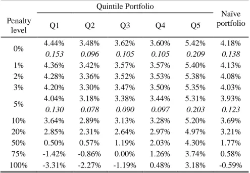
Figure 2, built with figures for a penalty level of 5% for disappearing funds, indicates that the final value of the highest quintile portfolio (Q5) is substantially higher than all others. We report in Table 10 detailed values of the returns on the whole period, for ten different levels of penalty. If we consider a reasonable penalty of 2%, the highest quintile provides a terminal value of 1,882, corresponding to a compound return of 5.38%, while the lowest (Q1) provides 4.28% (final value of 1,659). The compound return of the Q5 portfolio remains at 4.97% even when a (largely overestimated) penalty of 20% per delisted fund is applied, while it drops to 2.85% for Q1, which clearly indicates that the major source of performance difference between the portfolios lies in the capacity to anticipate a fund’s exit from the database.
[ Insert Table 10 approximately here ]
For comparison purpose, we also report the values for a naïve portfolio equally invested in all funds from the sample: its compound returns is hardly higher than the best from the portfolios in Q1, Q2, Q3, Q4, and largely inferior to the compound return of Q5.
The Sharpe ratios of the quintile and of the naïve portfolios, reported for two reasonable values of the penalty (0 and 5%), show that the highest quintile portfolio performs unequivocally best, according to the Jobson and Korkie (1981) test statistic.
3.5. Comparison with other predictor types
We now check the importance of our contribution, comparing the robustness of our results with models considering variables analyzed in previous papers, mainly the assets under management (AUM), age, and realized total returns.
We first consider the age and past returns (lagged 12 months) of the funds. We retrieve the inception date of 1,573 funds, forming a single sample28. Considering that persistence studies using these variables usually examine one-year or longer persistence, we apply the logistic regressions to predict each fund’s disappearance in the next twelve and eighteen months. We alternatively consider age and the logarithm of age. To make the estimation window consistent with the time frame of the computation of lagged returns, we restrict it to one year.
Table 11 shows that the age and returns are indeed predictive, but much less than a model building on past performance, contagion and frailty when their Somers’ D with similar estimation and forecasting windows are compared. The logarithm of the age reveals a slightly better predictor than the age itself. Past returns have a greater ability to predict a fund’s delisting than age. Combinations of age and returns improve further the Somers’ D, but still far from the values of model based on prior performance measures, contagion and frailty. A combined model, featuring all predictors (performance, contagion, frailty, age and returns) turns out to achieve the highest Somers’ D. Altogether, evidence presented in Table 11 suggests that prior performance encompasses much of the information embedded in a fund’s age and past returns, while the opposite is not true.
We consider next models based on the assets under management (AUM) of the funds. Over the considered period, we get 592,938 records from Bloomberg, concerning 1,108 funds. The series displays many anomalies and outliers. After a systematic check, we exclude abnormal data and remain with 585,515 observations. Most retrieved observations refer to the years 2001 or
28 For the purpose of comparing predictability for different model specifications, one having few variables (age,
AUM, returns) another one having many variables (performance measures), we do not need to split the sample in a
later. The proportion of dead funds is smaller in this sample than in the original one, i.e. 30%, compared to 42% in Table 2.
We first consider the prediction of disappearance using the AUM as the only forecasting variable. Table 11 reveals its low predictive power, displaying Somers’ D values of about 10%, at a similar level as age, and much weaker than 30% with a model consisting of performance measures29. Introducing the variables examined in previous section indicates limited complementarity. Altogether, they deliver Somers’ D around 20%. Models that combine performance measures and AUM improve the quality of the forecasts, although not to a substantial extent. Completing these variables with age and prior returns does not bring any noteworthy added value.
In sum, models based on performance measures have a predictive power largely superior to models using classical variables, like the AUM and the age of the funds. Adding them only slightly increases the power of the models based on performance measures.
4.Conclusion
Even though the central role of past performance has been emphasized as a determinant of the ability of a mutual fund to survive over time, the investigation of the dimensions of performance that influence this ability has been long neglected. Besides a fund’s excess returns or its intercept of multi-factor asset pricing models, very few alternative performance measures have been used to explain its likelihood to disappear. This lack of interest probably results from the scarce
29 We consider the variation of AUM in the last period (one year, six months, three months and one month): the
predictive power of this variation is null. This is consistent with Brown and Goetzmann (1995) who find that new
interest shown amongst scholars towards the development of new performance measures over that last two decades.
We believe that many fund managers do not only attempt to derive their performance from their generation of alphas over a standardized asset pricing model. In the context of hedge funds, which can be seen as laboratories of novel fund management techniques, Liang and Park (2010) document that alternative risk measures related to skewed and leptokurtic distributions of returns are indeed good predictors of the fate of a fund. Many of their managers exhibit differential skills in the management of their total, systematic or specific risks, and some of them address investors with various profiles. Naturally, they tend to be judged on the basis of their delivery of a consistent performance. The case for a wide array of performance measures as explanatory determinants of fund survivorship is, from our point of view, warranted.
Our paper has shown that our claim can be, to a reasonable extent, empirically validated. By a careful calibration and reduction of performance metrics, and by the integration of parameters quantifying the dependence in the individual liquidation times, our discriminant analysis shows a significant ability of past performance to predict future survival. Of course, these findings ought to be refined and many robustness checks can also be performed. In particular, as the proof of the pudding is in the eating, we have to carry out an out-of-sample analysis showing the actual consequences of conditioning portfolio allocation decisions to the suspicion of a fund’s disappearance. This is a central item in our research agenda.
References
Bollen, N.P.B., Busse, J.A., 2001. On the Timing Ability of Mutual Fund Managers. Journal of Finance 56, 1075-1094.
Bollerslev, T., Gibson, M., Zhou, H., 2011. Dynamic Estimation of Volatility Risk Premia and Investor Risk Aversion from Option-Implied and Realized Volatilities. Journal of Econometrics 160, 235-245.
Brown, S.J., Goetzmann, W.N., 1995. Performance Persistence. Journal of Finance 50, 679-698. Brown, S.J., Goetzmann, W.N., Park, J., 1997. Conditions for Survival: Changing Risk and the Performance of Hedge Fund Managers and CTAs. Unpublished Manuscript, Yale University. Bu, Q., Lacey, N., 2009. On Understanding Mutual Fund Terminations. Journal of Economics and Finance 33, 80-99.
Butera, G., Faff, R., 2006. An Integrated Multi-model Credit Rating System for Private Firms. Review of Quantitative Finance and Accounting 27, 311-340.
Cameron, A.C., Hall, A.D., 2003. A Survival Analysis of Australian Equity Mutual Funds. Australian Journal of Management 28, 209-226.
Carhart, M.M., 1997. On Persistence in Mutual Fund Performance. Journal of Finance 52, 57-82. Carhart, M.M., Carpenter, J., Lynch, A.W., Musto, D., 2002. Mutual Fund Survivorship. Review of Financial Studies 15, 1439-1463.
Chapman, L., Stevenson, M., Hutson, E., 2008. Identifying and Predicting Financial Distress in Hedge Funds. Working Paper, 28th International Symposium on Forecasting – Nice.
Chen, S.-N., 1982. An Examination of Risk-Return Relationship in Bull and Bear Markets Using Time-Varying Betas. Journal of Financial and Quantitative Analysis 17, 265-286.
Chen, N.-F., Roll, R., Ross, S.A., 1986. Economic Forces and the Stock Market. Journal of Business 59, 383-403.
Christopherson, J.A., Ferson, W.E., Turner, A.L., 1999. Performance Evaluation Using Conditional Alphas and Betas. Journal of Portfolio Management 26, 59-72.
Cogneau, P., Hübner, G., 2009. The (more than) 100 Ways to Measure Portfolio Performance - Part 1: Standardized Risk-Adjusted Measures. Journal of Performance Measurement 13, 56-71. Cogneau, P., Hübner, G., 2009a. The (more than) 100 Ways to Measure Portfolio Performance - Part 2: Special Measures and Comparison. Journal of Performance Measurement 14, 56-69. Coles, J.L., Daniel, N.D., Nardari, F., 2006. Does the Choice of Model or Benchmark Affect Inference in Measuring Mutual Fund Performance? Working Paper, Arizona State University. Cox, D.R., 1972. Regression Models and Life-Tables (with Discussion). Journal of the Royal Statistical Society B 34, 187-220.
Darolles, S., Gagliardini, P., Gouriéroux, C., 2014. Contagion and Systematic Risk: an Application to the Survival of Hedge Funds. Working Paper.
Duffie, D., Eckner, A., Horel, G., Saita, L., 2009. Frailty Correlated Default. Journal of Finance 64, 2089-2183.
EFAMA, 2012. International Statistical Release: Worldwide Investment Fund Assets and Flows, Trends in the First Quarter 2012, EFAMA, Brussels.
Elton, E.J., Gruber, M.J., Blake, C.R., 1996. Survivorship Bias and Mutual Fund Performance. Review of Financial Studies 9, 1097-1120.
Fama, E.F., French, K.R., 1993. Common Risk Factors in the Returns on Stocks and Bonds. Journal of Financial Economics 33, 3-56.
Ferson, W.E., Harvey, C.R., 1995. Predictability and Time-Varying Risk in World Equity Markets. Research in Finance 13, 25-88.
Harrell, F.E. Jr., Lee, K.L., Mark, D.B., 1996. Tutorial in Biostatistics - Multivariable Prognostic Models: Issues in Developing Models, Evaluating Assumptions and Adequacy, and Measuring and Reducing Errors. Statistics in Medicine 15, 361-387.
ter Horst, J.R., Nijman, T.E., Verbeek, M., 2001. Eliminating Look-Ahead Bias in Evaluating Persistence in Mutual Fund Performance. Journal of Empirical Finance 8, 345-373.
Hu, Y.-C., Ansell, J., 2007. Measuring Retail Company Performance Using Credit Scoring Techniques. European Journal of Operational Research 183, 1595-1606
Jensen, M.C., 1968. The Performance of Mutual Funds in the Period 1945-64. Journal of Finance 23, 389-416.
Jobson, J.D., Korkie, B.M., 1981. Performance Hypothesis Testing with the Sharpe and Treynor Measures. Journal of Finance 36, 888–908.
Kim, M.K., Zumwalt J.K., 1979. An Analysis of Risk in Bull and Bear Markets. Journal of Financial and Quantitative Analysis 14, 1015-1025.
King, M., Wadhwani, S., 1990. Transmission of Volatility between Stock Markets. Review of Financial Studies 60, 5-33.
Koenker, R., Hallock, K., 2001. Quantile Regression: An Introduction. Journal of Economic Perspectives 15, 143–156.
Laitinen, E.K., 1999. Predicting a Corporate Credit Analyst's Risk Estimate by Logistic and Linear Models. International Review of Financial Analysis 8, 97-121.
Liang, B., Park, H., 2010. Predicting Hedge Fund Failure: A Comparison of Risk Measures. Journal of Financial and Quantitative Analysis 45, 199-222.
Lobosco, A., DiBartolomeo D., 1997. Approximating the Confidence Intervals for Sharpe Style Weights. Financial Analysts Journal 53, 80-85.
Lunde, A., Timmermann, A., Blake, D., 1999. The Hazards of Mutual Fund Underperformance: A Cox Regression Analysis. Journal of Empirical Finance 6, 121-152.
Malkiel, B.G., 1995. Returns from Investing in Equity Mutual Funds 1971–1991. Journal of Finance 50, 549–572.
Massa, M., Patgiri, R., 2009. Incentives and Mutual Fund Performance: Higher Performance or Just Higher Risk Taking? Review of Financial Studies 22, 1777-1815.
Melnik, A.L., Plaut, S.E., 1996. Industrial Structure in the Eurocredit Underwriting Market. Journal of International Money and Finance 15, 623-636.
Newson, R., 2006. Confidence Intervals for Rank Statistics: Somers’ D and Extensions. Strata Journal 6, 309-334.
Ng, M.S.F., 2008. Development of a Forecasting Model for Hedge Fund Failure: A Survival Analysis Approach. Thesis, University of Sidney.
Niklis, D., Doumpos, M., Zopounidis, C., 2012. Combining Market and Accounting-Based Models for Credit Scoring Using a Classification Scheme Based on Support Vector Machines. Working Paper, Technical University of Crete.
Paul, P., Pennell, M.L., Lemeshow, S., 2013. Standardizing the Power of the Hosmer-Lemeshow Goodness of Fit Test in Large Data Sets. Statistics in Medicine 32, 67-80.
Pencina, M. J., D’Agostino, R.B., 2004. Overall C as a Measure of Discrimination in Survival Analysis: Model Specific Population Value and Confidence Interval Estimation. Statistics in Medicine 23, 2109-2123.
Rohleder, M., Scholz, H., Wilkens, M., 2011. Survivorship Bias and Mutual Fund Performance: Relevance, Significance, and Methodical Differences. Review of Finance 15, 441-474.
Sawicki, J., 2001. Investors' Differential Response to Managed Fund Performance. Journal of Financial Research 24, pp.367-384.
Sharpe, W.F., 1992. Asset Allocation: Management Style and Performance Measurement. Journal of Portfolio Management 18, 7-19.
Sirri, E.R., Tufano P., 1998. Costly Search and Mutual Fund Flows. Journal of Finance 53, 1589-1622.
Somers, R.H., 1962. A New Asymmetric Measure of Association for Ordinal Variables. American Sociological Review 27, 799-811.
Table 1. Summary statistics of the funds returns
Panel A – Statistics by currency of denomination
ALL CHF EUR GBP JPY USD
Nb. of funds 1,624 26 663 705 30 200
mean Nb. of obs. 555 556 558 560 597 520
Mean weekly return 0.090% 0.050% 0.054% 0.130% -0.015% 0.092%
Mean yearly return 4.70% 2.60% 2.83% 6.73% -0.79% 4.79%
Mean yearly std.dev. 20.6% 20.0% 20.9% 19.2% 22.0% 23.9%
Mean skewness -0.42 -0.48 -0.40 -0.45 -0.33 -0.40
Mean Exc. Kurtosis 3.92 5.56 4.32 3.45 2.96 4.20
% Jarque-Bera at 5% 95.69% 88.46% 97.13% 95.32% 86.67% 94.50%
Panel B – Statistics by country of incorporation
AT BE FR UK IT LU Others
Nb. of funds 58 89 178 695 114 405 85
mean Nb. of obs. 526 652 555 559 680 511 481
Mean weekly return 0.026% 0.083% 0.079% 0.130% 0.083% 0.047% 0.054%
Mean yearly return 1.36% 4.34% 4.12% 6.78% 4.32% 2.43% 2.80%
Mean yearly std.dev. 20.3% 22.3% 21.3% 19.3% 17.8% 22.6% 21.9%
Mean skewness -0.46 -0.59 -0.37 -0.45 -0.41 -0.38 -0.33
Mean Exc. Kurtosis 3.34 5.99 4.44 3.45 4.45 4.08 3.42
% Jarque-Bera at 5% 91.38% 100.00% 98.88% 95.25% 98.25% 94.32% 94.12%
This Table reports descriptive statistics for the linear returns of the 1,624 open-ended accumulation mutual funds with major or full allocation in equities. Prices are extracted for the period starting on Friday December 30th 1994 and ending on Friday January 8th 2010, from Thomson Reuters Datastream. Funds are grouped by currency of denomination (Panel A) and by country of incorporation (Panel B). The first lines report the numbers of funds, then the mean number of weekly observations. The following lines report the averages of the first four moments of the distributions, then the percentages of funds for which a Jarque-Bera test permits to reject the normality at a threshold of 95%. Currencies are: CHF = Swiss Franc; EUR = Euro (local currencies converted at parity before 1999); GBP = British Pound; JPY = Yen;
USD = U.S. Dollar. Countries are: AT = Austria; BE = Belgium; FR = France; UK = The United Kingdom; IT = Italy; LU = Luxembourg.
Table 2. Fund delistings per motive vs. country, currency and year
Panel A – Motives of delisting per currency and country
Currency Country
ALL CHF EUR GBP JPY USD AT BE FR UK IT LU Oth
merged 418 7 143 199 5 64 7 12 36 197 17 143 6 26% 27% 22% 28% 17% 32% 12% 13% 20% 28% 15% 35% 7% liquidated 257 4 127 82 5 39 12 1 25 77 2 90 50 16% 15% 19% 12% 17% 20% 21% 1% 14% 11% 2% 22% 59% inactive 82 0 17 59 0 6 2 1 8 59 0 9 3 5% 0% 3% 8% 0% 3% 3% 1% 4% 8% 0% 2% 4% delisted 12 0 0 11 0 1 0 0 0 11 0 1 0 1% 0% 0% 2% 0% 1% 0% 0% 0% 2% 0% 0% 0% ALL 769 11 287 351 10 110 21 14 69 344 19 243 59 47% 42% 43% 50% 33% 55% 36% 16% 39% 49% 17% 60% 69%
This Table reports the number of delisted funds, by delisting type: merging, liquidation, inactivity and other delisting. Panel A reports the ventilation according to the currency of denomination and to the country of incorporation. Panel B reports the number of delistings per year: the first delistings happened in 1997 and we ceased the reporting in July 2011, 18 months after the last available prices. Data are reported for 1,624 open-ended accumulation mutual funds with major or full allocation in equities, extracted for the period starting on Friday December 30th 1994 and ending on Friday January 8th 2010, Panel B – Motives of delisting per year
Year ALL 97 98 99 00 01 02 03 04 05 06 07 08 09 10 11 merged 418 2 1 13 15 38 37 113 70 16 12 18 10 10 37 36 liquidated 257 0 0 1 9 9 16 45 37 35 19 15 11 17 25 18 inactive 82 0 0 4 1 6 0 5 11 15 16 7 5 7 1 4 delisted 12 1 4 3 0 0 0 0 1 0 0 2 0 0 1 0 ALL 769 3 5 21 15 53 53 163 119 66 47 42 26 34 64 58
from Thomson Reuters Datastream. The date and the reason of the delisting are retrieved manually, mainly from Bloomberg.
Table 3. Summary of the selected performance measures by classes
Class Count Proportion
Market Timing Measures 15 26.8%
alphas 7 12.5%
gammas and delta 8 14.3%
Return-based Ratios 15 26.8% Gain-based Ratios 11 19.6% Return-based Differences 9 16.1% Preference Based 5 8.9% Gain-based Differences 1 1.8% Total 56 100%
This Table reports the classes of the 56 remaining measures, after the elimination of redundancies. This selection is obtained by considering the average of the 15 yearly matrixes of Kendall correlations between the 147 computed measures depicted in the Appendix; then, a stepwise elimination procedure keeps the set of measures whose two-by-two correlations do not exceed 85%. The denominations of the classes are based on Cogneau and Hübner (2009 and 2009a).
Table 4. Somers’ D statistic and number of variables in the model
Panel A – Modeling sample
Disappearance time T (years)
0.25 0.5 0.75 1 1.5 average Performance horizon h (years) 1 meas. only 0.319 0.303 0.301 0.290 0.280 0.299 meas. + fr. + ctg. 0.403 0.367 0.370 0.350 0.331 0.364 2 meas. only 0.347 0.331 0.351 0.355 0.353 0.348 meas. + fr. + ctg. 0.379 0.373 0.383 0.368 0.367 0.374 3 meas. only 0.402 0.396 0.418 0.414 0.403 0.407 meas. + fr. + ctg. 0.403 0.404 0.420 0.423 0.401 0.410 4 meas. only 0.434 0.424 0.421 0.407 0.398 0.417 meas. + fr. + ctg. 0.442 0.433 0.395 0.417 0.402 0.418
average meas. only 0.376 0.364 0.373 0.366 0.359 0.367
meas. + fr. + ctg. 0.407 0.394 0.392 0.389 0.375 0.392
Panel B – Validation sample
Disappearance time T (years)
0.25 0.5 0.75 1 1.5 average Performance horizon h (years) 1 meas. only 0.156 0.167 0.178 0.185 0.208 0.179 meas. + fr. + ctg. 0.278 0.263 0.246 0.266 0.246 0.260 2 meas. only 0.251 0.243 0.287 0.290 0.303 0.275 meas. + fr. + ctg. 0.336 0.329 0.323 0.309 0.323 0.324 3 meas. only 0.289 0.326 0.328 0.329 0.318 0.318 meas. + fr. + ctg. 0.311 0.334 0.335 0.333 0.319 0.326 4 meas. only 0.307 0.314 0.294 0.319 0.305 0.308 meas. + fr. + ctg. 0.320 0.303 0.323 0.325 0.299 0.314
average meas. only 0.251 0.262 0.272 0.281 0.284 0.270