Cartel pricing and the structure of the world bauxite market

CARTEL PRICING AND THE STRUCTURE OF THE WORLD BAUXITE MARKET

by

Robert S. Pindyck

Massachusetts Institute of Technology MIT-EL 77-005WP

March 1977

*

Prepared for the Ford Foundation World Commodities Conference, Airlie, Virginia, March 18, 1977. Support for this work came from the National Science Foundation, under Grant # GSF SLA75-00739, and from the World Bank. The author would like to express his appreciation to Ross Heide for his excellent research assistance, to Tom Cauchois of the World Bank for his help in assembling some of the data, and to Harold Barnett and James Burrows for their comments and suggestions.

I. Introduction

The future of the New International Economic Order depends to a great extent on the ability of less developed countries to follow in the steps of the OPEC countries and improve their terms of trade by cartelizing and increasing the prices of the basic commodities that they export. The argu-ment has been made, however, that the success of OPEC is an exceptional

phenomenon - that there is little potential for most LDC's to raise their export commodity prices through cartelization, either because substitutes for the commodities exist so that elasticities of demand are large, or because there are too many producing countries with differing interests to form a cohesive cartel. While this argument may be true for most commodities, it is probably not true for bauxite. In the two-year period January 1974 to January 1976, members of the International Bauxite Association (IBA) imposed tax

levies that increased the f.o.b. price of bauxite from around $8 - $12/ton to around $20 - $30/ton. It appears in fact, that the potential for percentage increases in profits is greater for bauxite than it is for oil3 If oil is an exception to the rule, bauxite may be an even greater exception.

1

This argument has been made by Krasner [9]. For an opposing view, see Bergsten [3 and Mikdashi [10]. For general discussions of cartel behavior and the potential impact on commodity markets, see the Charles River Associates study

[ 4] and McNicol [10].

Jamaica nationalized 51% of its bauxite-alumina companies, and paid for these with low interest notes. The price of Jamaican bauxite is net of the export

levy per ton, which is computed as (PAT) 20 0 0/4.3, where PA is the average price of aluminum per pound in the U.S., 4.3 is the number of tons of Jamaican bauxite that yield one ton of aluminum, and T is the levy, equal to .08 for

FY75-76 and .085 today. (This formula is applied to long tons of bauxiteJ) Since the price of aluminum is now about 37¢ per pound, the per ton Jamaican levy is about $14.60.

3_{An earlier study by this author [j5] computed for oil, bauxite, and copper,}

the ratio of the sum of discounted- profits for a monopoly'cartel to that for a competitive market. Using a 5% discount rate, the ratio was 1.63 for bauxite and 1.54 for oil (with a 10% discount rate, the numbers were 4.95 and 1.94). As we will see in this paper, recent increases in the price of energy give a bauxite cartel even more potential for price (and profit) increases.

The International Bauxite Association was formed in early 1974 by Jamaica, Surinam, Guinea, Guyana, Australia, Sierra Leone, and Yugoslavia. Since 1974 the Dominican Republic, Haiti, Ghana, and Indonesia also became cartel members,

so that in 1975 IBA accounted for 85% of total non-Communist world bauxite production. Admittedly the economic magnitude involved in IBA price increases have not been large; the value of IBA bauxite shipments rose from $.5: billion in early 1974 to about $1.2 billion in early 1976, as compared to an increase in OPEC oil revenues from $20 billion in 1973 to around $110 billion in 1976. On the other hand, these magnitudes are quite significant to the alumina and aluminum producing industries, and are politically significant in that they

raise the expectations of the other developing countries.

Table 1 shows, for 1966 and 1975, bauxite production and proved reserves for various producing countries. Note that the greatest change has been in the position of Australia, which is now the largest producer of bauxite, holds the largest proved reserve base, and has the most rapidly growing production capacity. (Observe that the production of the U.S. and the other non-cartel countries has remained about constant; the U.S. now imports about 90% of its consumed-bauxite and alumina.) As Barnett [2 ] points out, there are indications that Australia may be a weak link in the cohesiveness of IBA. Australia has not increased its tax as have the other cartel members, and has thereby moved from

4 a position of competitive disadvantage (because of distance) to one of advantage. Australia has recently been expanding its sales and relative share of the market

at the expense of the Caribbean countries, which have had constant or declining sales, and declining market shares. And the squeeze on the Caribbean countries may become tighter as Brazil begins to develop its potential reserves of bauxite. 41974 transport costs to the USA ranged from $1.00 to $6.00 per metric ton for

the Caribbean countries, but around $11.00 per metric ton for Australia. The tax levies of the Caribbean producers, however, have been considerably greater than these transport differentials. Source of data: Charles River Associates.

TABLE 1 - BAUXITE PRODUCTION AND RESERVES (Source of data: U.S. Bureau of Mines [16])

Cartel Members: Australia Jamaica Surinam Guinea Guyana Others Cartel total Non-Communist Market Countries: USA France Greece Other Market country total Total Non-Communist Production and Reserves Production (mmt) 1966 1975 1.8 20.7 9.0 11.4 4.5 4.9 3.1 9.0 2.9 3.2 4.1 6.0 25.4 55.2 1.8 1.8 2.8 2.5 3.2

}3.5

3.2

2.4 8.1 9.9 33.5 65.1 Proved Reserves (mmt) 1966 1975 3500 4500 600 1500 250 500 1200 4500 85 150 500 2500 6135 13650 45 40 70 40 } 520 2000 2000 635 2830 6770 16480 . . .

----There are two fundamental questions that are critical in assessing the future evolution of the world bauxite market. First, assuming that the existing configuration of the International Bauxite Association proved to be a stable one, what kind of pricing and output policies might the cartel follow, and how would these policies affect the world bauxite market? Second, to what extent is IBA likely to suceed as a coherent, stable, and enduring cartel?

One way to answer the first question is to determine what an optimal policy would be. This must be done in a dynamic context, so as to capture three

important aspects of the cartel pricing problem: the process of depletion of a finite (proved plus potential) reserve base, the slow adjustment over time of demand and supply to price changes, and the highly non-linear characteristic of bauxite demand. Although proved reserves of most cartel members would, last about 200 years at current production levels, reserves would last only 55 years if production grows by 4% per year, so that depletion should be accounted for. Dynamic adjustments of demand and supply must also be considered; bauxite supplies from non-cartel members can increase only slowly in response to price increases, so that a potential exists for large short-term gains to the cartel. Finally, any calculation of optimal cartel prices must account for the fact that the bauxite demand curve, while highly inelastic over a broad region, becomes almost infinitely elastic above a certain critical price level at which alternatives to bauxite become economical.

Answering the second question requires examining those factors that could lead to cartel instability. This includes differing production costs by different members, product heterogeneity across producers, and most important, the ability of one or more cartel members to earn higher revenues by undercutting the cartel

price and expanding production. Australia is the one member of the cartel for whom these factors are most likely to apply. Although production costs are about the same, transport costs are larger, and since transport costs vary

across consumers, this provides a means of undercutting. Also, since Australia has a rapidly growing capacity, it may be preferable for her to price and sell bauxite outside the cartel boundaries.

To provide some answers to both questions we extend the earlier work of this author 151 and calculate optimal cartel pricing policies using a simple optimal control model that captures the basic aspects of the pricing problem described above. These optimal policies are calculated for two alternative

configurations of the cartel. First, we assume that Australia remains a member of the cartel, and produces a constant share of cartel output. Next, we assume that Australia leaves the cartel and produces bauxite as part of the competitive fringe of price takers. We can then determine the resulting change in the net present value of the flow of cartel profits, and the change in the net present value of the flow of profits to Australia. This tells us, first, to what extent

it might be in Australia's interest to leave the cartel, and second, to what extent it is in the interest of the other cartel members to strike a bargain with Australia over some kind of output rationalization scheme.

The next two sections of this paper focus on the characteristics of the world bauxite market. First concentrating on bauxite demand, we will see that

the characteristics of the bauxite demand function (in particular the critical price at which alternatives to bauxite become economical) depends highly on world energy prices. We then examine the characteristics of bauxite production and reserves for the major producing countries. In Section 4 we specify a dynamic cartel pricing model, and use it to obtain optimal pricing policies

under two alternative assumptions - first that Australia is part of the cartel, and second that Australia is part of the competitive fringe. We also specify and solve a static equilibrium model in which Australia is part of the fringe, but has an infinitely elastic supply, and must adjust that supply optimally given the price reaction function of the cartel. These models will help us to determine whether it is in Australia's interest to leave the cartel, and how leaving the cartel might affect the price of bauxite.

2. The Demand for Bauxite

Up to some critical price, the demand curve for bauxite is highly inelastic, and this is one reason why a cartel like IBA has the potential to enjoy large monopoly profits. At a bauxite price of $10.00 per ton, bauxite itself repre-sents about 8 of the cost of producing aluminum, and if the price of bauxite doubles to $20.00 per ton, its share in aluminum production costs would only

5

rise to 12%. It is unlikely that the short-run and long-run price elasticities of aluminum demand are greater in magnitude than -0.2 and -1.0 respectively.6 Thus reasonable estimates for the short- and long-run price elasticities of bauxite deumad would be-around "-Q16 and -.08 respeetrely. -Asasiofg-tiat at

The cost of alumina represents about 30% of the cost of producing aluminum. At a $10.00 bauxite price, and using the Bayer process, bauxite represents about 26% of the cost of producing alumina (see Table 4). At a bauxite price of $20.00, bauxite represents 40% of the cost of producing alumina. In

fact only about 88% of bauxite and alumina consumed in the U.S. is used to to produce aluminum. About 6% is used in the production of chemicals, 4% in refractories and 2% in abrasives. Accounting for this, hever, would not change our elasticity estimates significantly.

I have seen no econometric estimates of the elasticities of demand for alumi-num. One would expect, however, these elasticities to be roughly comparable to those for copper demand. Fisher, Cootner, and Bailey [5] estimate the long-run elasticity of copper demand to be around -0.8, and Banks [1] estimates it to be -1.0.

current production levels, the production of

aluminum

from

alumina and the

pro-duction of alumina from bauxite both face roughly constant returns to scale,

the income elasticities for bauxite should be about the same as that for aluminum. A reasonable estimate for the long-run income elasticity of alumi-num demand would be 1.0. For purposes of analysis, we therefore take the short-run and long-run income elasticities of bauxite demand to be 0.2 and 1.0 respectively.

Should the price of bauxite rise above a certain level, it would become more economical to produce alumina from sources other than bauxite,

so that the demand for bauxite would become almost infinitely elastic. Clearly this critical price is a crucial determinant of the ability of a bauxite cartel to raise prices beyond their current levels, and it is

therefore worthwile estimating this price as accurately as possible.

Alumina (A1203) can also be produced from high-alumina clays, dawsonite,

alunite, and anorthosite, all of which are in great abundance in the earth's crust. Recently the U.S. Bureau of Mines estimated the fixed capital costs and annual operating costs of producing alumina from high-alumina clay, from anorthosite, and from bauxite [17]. There are some 18 alternative processes by which alumina can be produced from clay, but the most economical (over a

fairly wide range of factor input costs) is the hydrochloric acid-ion exchange

7

Again, no econometric estimates are available. If we use estimated income elasticities for copper, 1.0 would be appropriate.

8

Although there appears to be very little easily recoverable bauxite in the U.S., there are large amounts of high-alumina clays, dawsonite, alunite, and anorthosite. It is estimated, for example, that up to ten billion tons of high-grade clay (25% to 35% alumina) could be available in Arkansas, Georgia, and elsewhere in the U.S., and that one or two billion tons each of alunite

(37% alumina) could be available in Utah and Colorado, and large deposits of anorthosite have been found in California, Wyoming New York, and

process.9 There is only one economical process for producing alumina from anorthosite, and that is the lime-soda sinter process, and although this is a less economical way to produce alumina (given recent prices of clay and anor-thosite), it is close enough in cost to make it worth considering. The standard process by which alumina is produced from bauxite is the Bayer process.

The Bureau of Mines estimates are based on 1973 prices for factor

inputs, and I have updated these estimates to properly reflect 1976 prices.1 This updating has turned out to be critical, since the production of alumina from clay and anorthosite is much more energy-intensive than its production from bauxite, and energy prices have risen considerably in the last three

11

years. This has greatly increased the critical price at which bauxite is no longer economical.1 2

Annual operating costs for producing alumina from clay using the hydro-13

chloric acid-ion exchange process are shown in Table 2. Note that the

9_{Other clay-based processes that come close in cost are the nitric acid-ion}

process exthange and the hydrochloric acid-isopropyl etherreztz-etion process.

1. .- ; - - -* - ,

10My earlier study [15] is based on the 1973 data.

Given a particular process for producing alumina, the energy requirements per ton of alumina rise hyperbolically as the grade of the ore (percentage content of alumina) decreases. Clay and anorthosite have, on an average. much lower alumina content than bauxite. In addition, because of the par-ticular technologies that are available to extract alumina, for any given ore grade, use of anorthosite is more energy-intensive than use of clay, which in turn is more energy-.intensive than use of bauxite. See Page and

Creasey [12].

1 2_{Some of the chemical inputs needed to produce alumina from clay have also}

considerably risen in price.

1 3

In this process, clay is leached with hydrochloric acid to form a mixture of aluminum chloride and iron chloride. An amine-ion exchange procedure is used to remove the iron chloride, and the aluminum chloride is then crystalized and decomposed to alumina. For more details, see [17].

largest single factor cost is for natural gas, the wholesale industrial price of which has more than doubled since 1973. The costs for producing alumina

from anorthosite using the lime-soda sinter process are shown in Table 3. This process uses even more natural gas per ton of alumina, and is slightly more costly than the hydrochloric acid-ion exchange process. The difference is small enough, however, so that changes in the prices of raw materials could make it preferable. Finally, the costs for producing alumina from bauxite

using the Bayer process are shown in Table 4. Note that total operating costs are given as a function of the price of bauxite.

From Tables 2 and 4 we can easily compute the cross-over price at which clay becomes a more economical source of alumina than bauxite. That price is simply the solution to the equation

76.46 + 2.582P = 139.11 (1)

or P = $24.26 per short ton ($26.73 per metric ton). These calculations, however, are based on plants operating in the United States where natural gas prices (and energy prices in general) have been held below world market levels.

1 4

In this process anorthosite is blended and ground with limestone and soda ash, and then heated to form sodium aluminate and calcium silicate. The cal-cium silicate can be precipitated out by treatment with lime, the sodium aluminate is carbonated to precipitate alumina trihydrate, which is heated to form alumina. For details see [71?].

1 5

In the Bayer process, bauxite is heated with a caustic solution to form a solution of sodium aluminate, from which hydrated aluminum oxide can he precipated and calcinated to obtain alumina.

16I did not have similar data available for the factor cost of alumina pro-duction from bauxite or clay in other countries. Clearly these costs could differ greatly across countries.

Table 2

ANNUAL OPERATING COSTS, ALUMINA FROM CLAY USING HYDROCHLORIC ACID-ION EXCHANGE PROCESS1

Raw Materials:

Raw clay at $1.32/ton

Hydrochloric acid at $57.24/ton Organic solvent at $0.49/lb.

Chemicals for steamplant water treatment TOTAL . . . . Annual Cost (thousands of $) $2,324.50 2,805.00 750.00 103.00 $5,982.50 Cost/ton of alumina $6.64 8.01 2.14 0.30 $17.09 Utilities: Electricity at 1.7¢/kw-hr Water, process at 14.5¢/Mgal Water, raw at 1.45¢/Mgal

Natural gas at $1.10/MMBtu

TOTAL . . . . Direct labor: ($5.70/hr)

Plant maintenance:

Labor and supervision Materials

TOTAL . . . . Payroll overhead: (35% of payroll)

Operating supplies: (20% of plant maintenance) Indirect costs:2 (40% of direct labor and

Fixed Costs: maintenance)

Capital cost3 Taxes4

Insurance4

TOTAL . . . .

Total

₌₌₌

Oerating

_{= --- _====}

Costs

$ 798.00 75.00 323.50 14,551.00 $15,747.50 $ 1,964.00 $ 2,269.00 1,731.00 $ 4,000.00 $ 1,482.00 $ 800.00 $ 2,386.00 $13,613.00 1,361.00 1,361.00 $16,335.00

,$4867

00

$ 2.28 0.22 0.93 $41.58 $45.01 $ $ 5.61 $ 6.47 $ 4.94 $11.41 $ 4.23 $ 2.28 $ 6.81 $38.89 3.89 3.89 $46.67 $139.11

--Table 3

ANNUAL OPERATING COSTS, ALUMINA FROM ANORTHOSITE USING LIME-SODA SINTER PROCESS1

Raw materials:

Anorthosite at $3.31/ton Limestone at $1.45/ton Soda ash at $51.48/ton

Grinding material at $0.22/lb.

TOTAL . . . . Utilities:

Electricity at 1.7 cents/kW-hr. Water, process at 14.5¢/Mgal Water, raw at 1.45¢/Mgal Natural gas at $1.10/MMBtu

TOTAL . . . . Direct labor: ($5.70/hr.)

Plant maintenance:

Labor and supervision Materials

TOTAL . . . . Payroll overhead: (35% of payroll)

Operating supplies: (2n0 of plant maintenance) Indirect costs:2(40% of direct labor and

maintenance) Fixed costs: Capital cost3 Taxes4 Insurance4 TOTAL . . . . Annual Cost (thousands of $) $5,632 4,403 1,531 695 $12,261 $ 4,224 958 21 16,727 $21,930

$

2,045

$ 1,476 984 $ 2,460 $ 1,232 $ 492 $ 1,802 $ 8,645 865 865 $10,375 Cost/ton of alumina $16.09 12.58 4.38

1.99

35.04 $12.07 2.74 0.06 47.79 $62.66 $ 5.84 $ 4.22 2.81 $ 7.03 $ 3.52 $ 1.41 $ 5.15 $24.70 2.47 2.47 $29.64 $52 597_=w=nrr

Table 4

ANNUAL OPERATING COSTS, ALUMINA FROM BAUXITE USING THE BAYER PROCESS1

Annual cost

Raw materials: (thousands of $)

Cost/ton of alumina Bauxite at $P/ton

Limestone at $1.45/ton Soda ash at $51.48/ton Starch at $130/ton

TOTAL . . . . Utilities:

Electricity at 1.7 cents/kW-hr. Steam, 300 psig, at $1.80/Mlb Water, cooling, at 2.9¢/Mgal Water, process, at 14.50/Mgal Natural gas at $1.10/MMBtu

TOTAL . . . . Direct labor:($5.70/hr)

Plant maintenance:

Operating supplies: (15% of plant maintenance) Indirect costs:2 (50% of direct labor and

maintenance) Fixed costs:

Capital cost3

Taxes and insurance4

TOTAL . . . .

Total Operating Costs

$903.7xP 75 1351 274 $1700+903.7P $ 425 4,961 28 102 1,867 $7,383 $2,304 $2,218 $ 333 $2,261 $8,811 1,762 $10,573

$27,872+903.7P

1==r====== $2.582xP 0.21 3.86 0.78 .;$4.85+2.582P $ 1.21 14.17 0.08 0.29 5.33 $21.08 $ 6.58 $ 6.34 $ 0.95 $ 6.46 $25.17 5.03 $30.20

$76.46+2.582P

_ __

NOTES TO TABLES 2, 3, and 4

All figures are in 1976 dollars, and are in terms of short tons. To convert to equivalent metric ton figures, increase all numbers by 10 percent. For each process, figures are based on a plant with capacity of 1000 tons of alumina per day, and an average of 350 days of operation per year over the life of the plant (allowing 15 days downtime per year for inspection, main-tenance, and unscheduled interruptions). The numbers represent a cost updating of the 1973 figures assembled by the U.S. Bureau of Mines [17]. Changes in the unit costs of materials, utilities, labor, and capital are based on data from the Survey of Current Business, and are summarized below:

Input 1973 cost 1976 cost

Raw clay $1.00/ton $1.32/ton

Anorthosite $2.50/ton $3.31/ton

Hydrochloric acid $27.00/ton $57.24/ton

Limestone $1.00/ton $1.45/ton

Price index, other chemicals 1.00 2.12

Electricity 1.0¢/kW-hr. 1.7¢/kW-hr.

Steam $0.90/Mlb $1.80/Mlb

Process water 10¢/Mgal 14.5¢/Mgal

Natural gas $0.50/MMBtu $1.10/MMBtu

Labor $4.50/hr $5.70/hr.

Price index, capital assets 1.000 1.336

2Indirect costs include expenses for control laboratories, accounting, plant protection and safety, and plant administration. Research costs, and company

administrative costs outside the plant are not included.

3

Assumes a 10% cost of capital, and ignores replacement costs.

It is quite possible that through deregulation natural gas prices in the U.S. will increase significantly in the near future, and this will change the cross-over price. It is reasonable to assume a further doubling of the wholesale in-dustrial price of natural gas to $2.20 per MMBtu (putting the price abbut equal to the world market price of oil on a Btu equivalent basis). It is also reasonable to assume that should this happen the cost of steam (used in the Bayer process) would increase by 502 as well.1 7 In this case the cross-over price is the solution to equation

88.88 + 2.58P - 180.69

(2)

18

or P $35.56 per short ton ($39.19 per metric ton). Thus higher energy prices will greatly extend the inelastic region of the bauxite demand durve.

Clearly the demand function for bauxite will differ across consuming regions. For purposes of crude analysis, however, it is useful to specify a single function for total non-Communist bauxite demand. Using the short-run and long-short-run price elasticities of -.016 and -.08 at a price of $15.00 per metric ton and total demand of 65.5 million metric tons (equal to actual 1974 demand), using short-run and long-run income elasticities of 0.2 and 1.0, and assuming 3% real growth in the aggregate GNP of consuming countries, we can specify the following bauxite demand function:

TDt [1.048 - .06986Pt + 13.1(1.03)t]e (Pt/ + .8TDt- (3)

where TD is total demand in millions of metric tons, and P is the critical price

17I am assuming here that natural gas currently provides about half of the boiler fuel used to generate steam. I have not, however, been able to check this assumption.

1 8

Since natural gas prices are higher in other alimina-producing countries, the current cross-over price probably varies from $24.26 per short ton in the U.S. to nearly $35.00 in some European countries.

at which alternatives to bauxite become economical. We will analyze the effects of energy prices on potential bauxite cartel behavior by using two alternative values

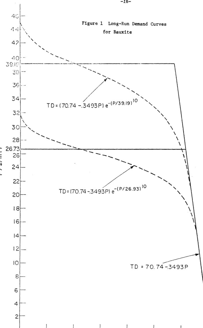
for P, $26.73 and $39.19 (both per metric ton). By attaching a large enough exponent to the term (Pt/P), we can achieve an arbitrarily close approximation to a piecewise linear demand function. In fact we would expect demand to start falling off at prices somewhere below the critical price P (if for no other reason than in anticipation of future price increases), and demand to be small but not zero at higher prices, so we choose 10 as the exponent. Long-run bauxite demand functions for the two alternative values of P are plotted in Figure 1.

Z_, Bauxite Production and Reserves

The ability of IBA to increase its profits as it raises price depends partly on the supply response of non-IBA countries, and, should it decide

to leave the cartel, Australia's ability to increase its output over time

in response to price increases. Unfortunately the determinants of bauxite sup-ply are complicdated and difficult to describe in the context of a simple model.

Some bauxite producers are parts of the major vertically integrated aluminum companies, the number of producers in each country varies across countries, and changes in supply are brought about by other factors besides changes in price. The potential (and proved) reserves of bauxite in the major producing

countries are large, so that conceivably any amount of bauxite could be pro-duced, given the time required to increase capacity.

Looking at the pattern of bauxite production in different countries over the last decade or so affirms that there is no simple supply function that can be easily identified. Production levels for a number of countries are shown

Figure 1 Long-Run Demand Curves for Bauxite N~ IN N\

TD

(70.74

-.34(P/

3 9 9

)

)

I0

T D

=

(70.74

-3

493 P)

e

-N 'x

TD = (70.74 -. 349

3P)

e

- (P

_/26

'

₉₃₎₁₀

TD

= 70.

74-3493P

i -7 _{. -}C

26

\

22

20

18 14

12

10

a

6

4

4,

_I,

I

for the last 15 years in Table 5. Bauxite prices remained roughly constant from 1960 to 1971 (and were probably close to average production costs plus average amortized exploration costs). During that time there was little change in U.S. production, production in France increased by about 50X, production in Guyana, Surinam and Jamaica about doubled, but production in Australia increased from zero to about 14 million metric tons per year. Since 1971, and in particular over the last two years, bauxite ptices have doubled or tripled. Production in the U.S., France, Jamaica and Surinam remained con-stant or declined slightly, production in Guyana declined by about 35%, while production in Australia increased by another 40% between 1972 and 1975. There is no overall pattern of supply response to price changes that can be discerned here.

Bauxite production costs also vary to a considerable extent across coun-tries, although 1976 average production costs are fairly uniform at around $6 to $7 per metric ton for those IBA countries with large proved reserves. Average 1976 production costs (including fixed charges) for Jamaica were

recent-19

ly estimated to be $6.31 per metric ton. Production costs in 1974 were es-timated to be $6.00 per metric ton in Australia, $6.00 in Guyana, $5.00 in

20

Surinam, $5.90 in Haiti, and $4.00 in the Dominican Republic. 1976 prod-uction costs for the large Guinea-Boke project (current capacity about 6 million tons per year) are much larger - about $11.00 per metric ton.2 1

Given the regional variation in production costs, reserves (see Table 1), current and planned -capacity, and transportation costs, it seems clear that

1 9

Figures obtained from conversations with World Bank officials.

20

Source: Charles River Associates 21

Source: Conversations with World Bank officials. In 1968 costs were projected to be about $5.40 per ton, but since then labor costs and

TABLE 5 - BAUXITE PRODUCTION*

(quantities in thousands of metric tons)

Australia O

50

350 889 1158 1800 4169 4880 7792 9200 12,343 14,205 15,800 17,535 20,700 Other Free World 7452 7128 7379 7879 9080 10,700 10,200 11,400 12,200 13,600 14,700 15,000 11,900 17,900

20,600

* Source of data: U.S. Bureau of Mines [18] U.S. 1228 1369 1525 1601 1654 1796 1654 1665 1843 2082 1988 1812 1880 1950 1800 1961 1962 1963 1964 1965 1966 1967 1968 1969 1970 1971 1972 1973 1974 1975 Guyana 2374 2690 2210 2468 2638 2860 3328 3490 3700 4490 3757 3668 3224 3100 3200 France 2148 2127 1971 2387 2610 2760 2745 2756 2729 2940 3066 3203 3084 2863 2500 Jamaica 6663 7435 6903 7811 8514 8950 · 9121 8391 10,333 11,800 12,565 12,345 13,385 15,086 11,400 Surinam

3351

3202 3427 3926 4291 4520 5200 5484 5451 5257 6162 6800 6580 7000 4900 . .

any accurate projection of bauxite supply would require a model with a high degree of regional disaggregation. However, in order to analyze in at least rough terms the potential behavior of IBA, we must make some assumptions about average production costs and aggregate supply elasticities. Average 1976 production costs for IBA could reasonbly be taken to be about $7.00 per metric ton, although we must recognize that these costs will increase slowly over the years as higher grade reserves are depleted. We aggregate non-IBA countries together and view them as competitive price takers with a long-run

supply of elasticity of 2. This elasticity may seem large given some of the figures in Table 5, but we assume a ten-year mean adjustment between the

short-and long-run.

We must also account for reserve depletion in both IBA and non-IBA countries. 1975 IBA reserves were about 12,400 million metric tons; we assume that IBA pro-duction costs rise hyperbolically from $7 per ton as these reserves are depleted, i.e., IBA costs are given by 86,800/Rt, where Rt is reserves in mt. Averaging

over all countries, reserves are about 200 times current production levels. As these reserves are used up, new ones will be found, but at higher cost, so that the supply curve for the competitive fringe will move to the left over time. We assume that after all current reserves are depleted, supply would be about

35% of its current level, given the current price.

Our assumptions about supply elasticities and the shift in supply as re-serves are depleted lead to the following supply function for the non-IBA pro-ducers:

St (-1.1

+

.1467t)(1.005)-CSt/11

+ .90S_

1

(4)

where CS is cumulative supply (zero in 1975), and the initial supply level is 11 nmt/yr. At a price of $15 the long-run supply elasticity is then 2.0.

4. Potential Pricin& Policies for IBA.

We can now lay out two versions of a simple aggregate model of the world bauxite market, and use them to examine potential cartel pricing policies.

In the first version Australia remains part of IBA:

TD _Tt = [1.048 - .06986P + 13.1(1.03)] e (. _{t +} + _'80TDt 8 0 _{t-1 (5)}(5) St = (-1.1 + .14 6 7Pt)(1.005) -CSt/ll + .90St l (6) CSt = CSt-l t (7) Dt Tt - St (8) Rt =Rt- -Dt (9) N 1 86,000 MaxW = [ t Rt t (10)

t~ 6)

U+Ot

t

(10)

The equations for total demand (TD) and competitive supply (S) were discussed above, CS is cumulative competitive supply, D is the net demand for IBA bauxite, R is IBA reserves, and W is the sum of discounted profits. Quantities are in millions of metric tons, and prices in 1976 dollars per metric ton. We solve this model (i.e. determine the price trajectory that maximizes W) using a gen-eral nonlinear optimal control algorithm developed by Hnyilicza [7]. Initial conditions for the solution correspond to actual 1974 data: TDo - 65.5 mmt/yr, SO = 11.0 mmt/yr, R = 12,400 mat, and CSo = 0. The time horizon N is large enough (60 years) to approximate an infinite-horizon solution, and the discount rate 6 is chosen to be 5%.

In the second version of this model, Australia is included as part of the competitive fringe. This involves modifying the supply equation,

St

(-2.9

+

3867Pt)(1.005)

CSt/29

+ .90St₁

(6a)

and the cartel objective function, N 1

N

1E

- 5 8

,

1 0 0

]D

MaxW i Z (i+6)t [Pt - _tR(10aR

_~]t-l

t

The initial conditions are now TD = 65.5, S 29.0, R = 8300, and CS - 0.

0 0 0 0

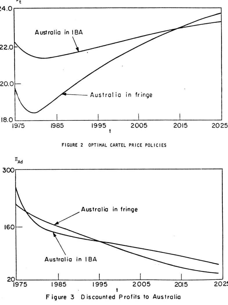
The solutions to both versions of the model are given in Table 6, and the optimal price trajectories and profits to Australia are shown graphically in Figures 2 and 3. The initial decline in prices reflects the ability of the cartel to enjoy large short-run profits by taking advantage of the lags in the response of total demand and competitive supply to higher prices. In both cases prices gradually approach the limit price ($26.76) at which alternatives to bauxite become economical. Comparing the price trajectories for the two ver-sions of the model, we see that prices are lower for about the first 25 years, but later higher, when Asutralia is part of the competitive fringe. If the

fringe becomes larger at the expense of the cartel, the optimal price trajec-tory would become closer to ;-at would prevail in a competitive market, and for an exhaustible resource the monopoly price is initially higher, and later

lower, than the competitive price.

It is not clear from these results whether it would pay for Australia to leave the cartel. Australia's sum of discounted profits for the first 20 years

TD 65.50 63.16 61.86 61.35 61.43 61.95 68.33 77.79 88.99 101.77 116.26 132.62 151.04 171.80 195.64 D 54.50 51.12 48.95 47.69 47.13 47.11 51.71 60.34 71.21 83.97 98.61 115.23 113.96 115.06 179.27 R 12400.00 12348.90 12299.90 12252.20 12205.10 12158.00 11911.00 11627.70 11294.10 10900.50 10437.50 9895.42 9263.97 8531.89 7685.52 d 790.22 690.44 619.06 567.26 529.11 500.52 427.07 391.92 363.35 335.13 306.05 275.95 244.80 212.39 177.73 - Australia D 36.50 33.89 32.39 31.74 31.68 32.04 36.97 44.52 54.01 65.38 78.55 93.38 109.60 126.85 145.36 in Compet R 8300.00 8266.12 8233.72 8201.98 8170.30 8138.26 7964.76 7758.07 7507.75 7204.32 6838.62 6402.00 5886.95 5287.55 4598.61 itive Fringe IT *** d 438.21 369.98 325.43 297.32 280.23 270.17 257.50 255.66 251.61 243.68 231.35 214.42 192.79 166.26 133.84 Discounted ** Discounted profits to profits to

cartel including Australia (millions Australia

of 1976 dollars)

Discounted profits to cartel, excluding Australia P 1975 1976 1977 1978 1979 1980 1985 1990 1995 2000 2005 2010 2015 2020 2025 22.22 21.92 21.70 21.54 21.44 21.38 21.41 21.64 21.90 22.15 22.40 22.64 22.88 23.10 23.23 ** 1 Ad 260.99 228.04 204.46 187.35 174.75 165.31 141.05 129.44 120.01 110.69 101.08 91.14 80.85 70.15 58.70 2 1975 1976 1977 1978 1979 1980 1985 1990 1995 2000 2005 2010 2015 2020 2025 P 19.61 19.07 18.69 18.47 18.40 18.44 19.21 20.02 20.72 21.32 21.86 22.37 22.87 23.35 23.72 Version TD 65.50 64.22 64.46 64.83 65.59 66.64 74.28 84.11 95.42 108.10 122.14 137.46 153.90 171.18 189.53 ** HAd 215.50 207.59 199.09 191.43 185.09 179.89 159.98 140.07 119.41 99.55 81.62 66.13 53.15 42.43 33.46 . . . . -:

-Pt

1975

1985

1995

2005

2015

2025

t

FIGURE 2 OPTIMAL CARTEL PRICE POLICIES

n1Ad

t

Discounted Profits to

25

>4.U

22.0

20.0

IR8. I

F igure 3

Austraolia

22

either time horizon the difference is small. Since few governments have planning horizons longer than ten years, the shorter time horizon is probably more meaningful, and we might argue that it is marginally in Australia's in-terest to leave the cartel.

A key question here is the extent to which Australia can increase its out-put without incurring large increases in marginal and average cost. We assumed above that as part of the fringe Australia would have the same long-run supply elasticity (2.0) as the other competitive producers. It is likely, however, that Australia's supply is much more elastic than that of other countries.

It would be reasonable, in fact, to assume that Australia's supply is infinitely elastic, and that it can produce almost any amount of bauxite at a constant average cost of $7 per ton.

This assumption leads to a quite different model of the bauxite market. As part of the fringe, Australia would be a price taker as before (IBA would still set price to maximize its profts), but would determine its quantity -given the expected price reaction of the cartel - to maximize its own profits. We have in effect a Stackelberg model of market behavior, and we can solve this model if it is expressed as a static long-run equilibrium approximation to the model of equations (5)-(10).

We write the static (long-run) total demand function for 1980 as 10

TD (77.29 - .3493P) e- ( 0 3 7 4 1 P) ' (11)

A22istralia makes larger profits during the first two years as part of IBA since as part of the fringe its awn supply can adjust only slowly in response to price increases. In the next twenty years its profits are lower as part of IBA since net cartel demand is reduced as the fringe expands its output. Higher output as part of the finge during the first twenty years, however, means lower output later as reserves are depleted.

and the supply function of the competitive ftinge, excluding Australia, as

S -11.0 + 1.467P (12)

Denoting Australia's output by Qa, the net demand to the cartel is then

D = TD - S - (13)

We assume that the cartel adjusts price in response to Australia's output, which it takes as given:

Cartel: Max n = (P-7)(TD(P) - S(P) - Qa) P

(14)

Substituting (11) and (12) into (14), we have the following approximate

re-acion n fr the cartel:unc 23

action function for the cartel:

P = 28.06 - .28 Qa (15)

We now assume that Australia chooses its profit-maximizing output given this reaction function:

Australia: Max Ia

_aa

= (28.06 - .28Qa - 7)Qa

_a

(16)

This implies Qa = 37.6 mmt/yr and P $17.53.

2 3

The exact reaction function is found by solving the following equation for P in terms of Qa:

21.27 - 2.93P + e

-(.03741P) 10 (.03741)l(3.P 797)

!-(.0374 P) [79.74 - .70 + (.03741P) (3.5? - 797) + 202 (.03741P)9 = Qa

However, for prices less than $20 (Qa greater than 28 mmt/yr), equation (15) is correct to within 2% of the true price.

In Table 7 we summarize the 1980 equilibrium bauxite prices, undiscounted profits, demand and supply implied by the three alternative sets of assumptions analyzed above. Cases 1 and 2 correspond to the dynamic optimal pricing model, first with Australia in IBA, and then with Australia in the finge, with

a long-run supply elasticity of 2.0. Case 3 corresponds to the static model where Australia is in the fringe, but has an infinite long-run supply elasticity.

Note that Australia's profits in Cases 1 and 2 are nearly the same, but are considerably increased in Case 3. Comparing Case 3 with Case 1, we see that if Australia can increase production with no increase in average cost, it can almost

double its profits by more than doubling its output. Profits to the other car-tel members fall by more than half, but it is still optimal for the carcar-tel members to maintain a price that is only about $4 lower.

Australia's actual supply characteristics probably lie somewhere between the representations in Cases 2 and 3. It is likely that Australia could greatly increase its output over the next five years, but its average cost might rise by a few dollars. If this is the case, it indeed seems in Australia's interest

to leave the cartel - and it also seems in the interest of the other cartel mem-bers to make whatever adjustments are necessary to induce Australia to remain

in the cartel. Such adjustments would probably mean allowing Australia to con-siderably increase its market share at the expense of the other members. Higher profits could then be made by everyone by maintaining a higher price. If

Australia's output share of IBA production were 67%, as in Case 3, but the cartel maintained a price of $21.44, as in Case 1, Australia's profits would rise to

$456 million, and profits to the other members of IBA would rise to $225 million. (See Case 4 in Table 7.) Of course we have no way of knowing whether this

14 C14 <rj Cn r-q

C,-0

0O H Un 0 H H 0o r-00 -H~ H r-i ?-00 %O ,0 co Hn -q 00 cn Ln -T *n %7 Hr H4 C,

'\o

cn '0 H r- 0 , -Ln O O n * %Q I U) Ln e4 CN 00 00 Hq r-U, m, O U, r4 .-U) , H aD Ln ON N- 0 H- C qc --

T

0

1

-

Cm

Ul) CT Lr) -T~~~~~~UC' H U, H U,~~~~~~~~~~~V 10 M% CNI C' H HLn '4 C14 C r-I rl %O --t C14 C 0 I H w C

XH

¢K 4Jqw

4:

to

r.

PcW -lO 0 -H III 0 < O 11: I 0 4-i o ci 0 0 0 54 r 0.4 0

p

-x H i 44 l U) P

0 x

:

$-4 0-c p-I 0 Qo S

~4J

-r4 rn H 0 0w 0 -H 0 ' * IH

u 40

H- -9 ocb t u o X p4 r-P4 I to 4 w U 0 -C U)4* 4J* -H O P -H r-I -Wl₀ }w l.J U 0_I 0 -H r-i 0 '-4 -I C", w U 0 U) 0, U 0 -H H JJ 1 C1 Cu₀ U) 0 uu₎ U

0

O0 0 H 0 _a a a

8

II 0 H H rD 0 II

0

H_1. w_S= 1: to C:r -H 14 0 AJ-Ug H H U) Q-a: C 4-r__F 9, ff 0 -4

~41

co 0 w 1-m 0 4-4 0 U) w 0 -H 41 0 -H

_a,

H H I r-0 H r-q ·t4 Cc E 4 4~ o4 4) I4J rn U)₀ H AJ 01 a rl 0 El a) A) U) ,-4 ,-4 O r cn O

I

-H₀ 1 U) a, 0d O 4I .H 0 o '4 0 U) a4 C, "-_H

a

'o_I l 3z I 4C K I IC _.K K __

agreement were to occur, the division of output among the cartel members would depend on relative bargaining power, and might be somewhere in between the out-put shares of Cases 1 and 3.24

5. Concluding Remarks

Given IBA's current configuration, its optimal price of bauxite today is about $22, and this is quite close to the actual price. IBA may or may not know that it is now pricing bauxite optimally, but if the cartel remains in its pre-sent form and continues to price optimally, the (real) price of bauxite would fall slightly to ust over $21 in 1980, and then rise by no more than 0.2% per year for the next few decades.

Should Australia leave the cartel, however, the price of bauxite would probably fall by $3 or $4. There is a strong incentive for Australia to leave,

since by doing so it could nearly double its profits. Although the other car-tel members also have an incentive to keep Australia in the carcar-tel, their bar-gaining power is limited, and any agreement (over output shares) acceptable to Australia would still leave the rest of IBA with greatly reduced profits.

Our calculations of optimal prices were based on certain assumptions about energy prices. We have seen that an increase in energy prices (in particular the price of natural gas) would result in an extension of the inelastic region of the total demand function for bauiite, and this could considerably increase the optimal cartel price.(whether or not Australia is a member.of the cartel). A doubling of the wholesale price of natural gas, for example, would probably

24

Nash bargaining theory provides a framework for determining relative bar-gaining power and a likely division of output. For an application of this theory o the analysis of the OPEC oil cartel, see Hnyilicza and Pindyck [8].

increase the optimal price to about $30 if Australia is in IBA, and about $25 otherwise. On the other hand, we have also assumed that no new major pro-ducers of bauxite enter the world market in the coming years. By 1982 Brazil might have the capacity to produce some 4 mt of bauxite per year at a cost of about $6 per ton, and this could significantly reduce any optimal cartel price, particularly if Australia is not in the cartel. Thus our analysis of optimal cartel prices can only be conditioned on the future of such exogneous factors as energy prices and entry of new producers.

The analysis i this paper is based on an extremely crude and over-simpli-fied model of the world bauxite market. The main shortcoming of our model is that it ignores the important regional characteristics of the bauxite market. The cost and other determinants of bauxite production, and the quality of bau-xite produced, vary across regions, as do the nature of the contracts that producers write with alumina and aluminum producing companies. And we have ignored transportation costs, which are a large component of the c.i.f. cost of bauxite, and would be a major factor in Australia's pricing and output de-cisions. Better projections of prices and output require a detailed and regionally disaggregated model of the world bauxite market. The construction of such a model should be an objective of future research.

[1] Banks, F.E., The World Copper Market, Ballinger, Cambridge, Mass., 1974. [2] Barnett, H.J., "Notes on the Bauxite Trade," unpublished paper, Woodrow

Wilson Center, Smithsonian Institution, Washington, D.C., June, 1976. [3] Bergsten, C.F. "The Threat from the Third World," Foreign Policy, Vol.

11, 1973, pp. 102-124.

[4] Charles River Associates, "A Framework for Analyzing Commodity Supply Restrictions," Report # 220, August 1976.

[5] Fisher, F.M., P.H. Cootner, and M.N. Baily, "An Econometric Model of the World Copper Industry," Bell Journal of Economics and Management Science, Autumn, 1972 (Vol. 3, No. 2).

[6] Goudarzi, G.H., L.F. Rooney, and G.L. Shaffer, "Supply of Nonfuel Minerals and Materials for the United States Energy Industry, 1975-90," U.S.

Geological Survey Professional Paper 1006B, 1976.

[7] Hnyilicza, E., "OPCON: A Program for Optimal Control of Nonlinear Sys-tems," M.I.T. Energy Laboratory Report, May 1975.

[8] Huyilicza, E., and R.S. Pindyck, "Pricing Policies for A Two-Part Ex-haustible Resource Cartel: The Case of OPEC," European Economic Re-view, August, 1976.

[9] Krasner, S.D., "Oil is the Exception," Foreign Policy, No. 14, 1974, pp. 68-84.

[10] McNicol, D.L., "Commodity Agreements and the New International Economic Order," California Institute of Technology, Social Science Working Paper No. 144, November 1976.

[11] Mikdashi, Z., "Collusion Could Work," Foreign Policy, No. 14, pp. 57-68. [12] Page, N.J., and S.C. Creasey, "Ore Grade, Metal Production, and Energy,"

U.S. Geological Survey, Journal of Research, Vol. 3, No. 1, January 1975. [13] Patterson, S.H. "Bauxite Reserves and Potential Aluminum Resources of the

World," U.S. Geological Survey. Bulletin 1228, 1967.

[14] Patterson, S.H., and J.R. Dyni, "United States Mineral Resources: Alu-minum and Bauxite," U.S. Geological Survey Professional Paper 820, 1974.

[15] Pindyck, R.S., "Gains to Producers from the Cartelization of Exhaustible Resources," M.I.T. Energy Laboratory Working Paper No. 76-012WP, May 1976.

[16] U.S. Bureau of Mines, Commodity Data Summaries, Washington, D.C., various years.

[17] U.S. Bureau of Mines, Information Circular No. 8648, "Revised and Up-dated Cost Estimates for Producing Alumina from Domestic Raw Materials," by F.A. Peters and P.W. Johnson, 1974.