Efficient Path Planning for Nonholonomic Mobile Robots
St´ephane Lens
1and Bernard Boigelot
1Abstract— This work addresses path planning for nonholo-nomic robots moving in two-dimensional space. The problem consists in computing a sequence of line segments that leads from the current configuration of the robot to a target location, while avoiding a given set of obstacles. We describe a planning algorithm that has the advantage of being very efficient, requiring less of one millisecond of CPU time for the case studies that we have considered, and produces short paths. Our method relies on a search in a Voronoi graph that characterizes the possible ways of moving around obstacles, followed by a string-pulling procedure aimed at improving the resulting path.
I. INTRODUCTION
We consider the general problem of planning the motion of an autonomous nonholonomic robot in two-dimensional space, the goal being to reach a given configuration while avoiding some set of obstacles. For many applications, the ability of the robot to react quickly is crucial, and a strong emphasis must be placed on the efficiency of path planning, which often has to be carried out with the limited amount of computing power available on the robot. The objective is then not to find an optimal solution, but to develop a method that can very quickly synthesize a trajectory for reaching the target in acceptable time, and that is consistent with the physical limitations of the robot (e.g., sufficient clearance is ensured with respect to obstacles, speed and acceleration bounds are respected at all times). In addition, in order to be able to deal with dynamic environments, absence of any preprocessing of obstacles information is preferred.
Our approach to motion planning consists in dividing the problem in two major steps. The first one is aimed at finding a path that avoids obstacles and manages to reach the destination. Such a path takes the form of a sequence of straight line segments that clears the obstacles at a specified safety distance. The second step is to convert this path into a smooth trajectory that can be followed by the robot, taking into account its physical constraints.
In this paper, we focus on the first step, introducing a method for computing piecewise linear paths that lead from an origin to a destination while avoiding some set of obstacles with a given clearance. We consider differential drive robots, but our results are also applicable to tricycle platforms. This work has been motivated by the Eurobot2
contest, in which autonomous mobile robots have to compete against opponents in a small game area strewn with obstacles. This application requires, by nature, a high level of reactivity, which can only be achieved with fast
1Montefiore Institute, B28, University of Li`ege, B-4000 Li`ege, Belgium.
{lens,boigelot}@montefiore.ulg.ac.be
2http://www.eurobot.org/
trajectories, and low computation times for generating them. Our solution has been successfully implemented in the robots that we have built for this contest, together with the method described in [15] for carrying out the second step. In this setting, the main advantage of our approach, besides its efficiency, is that it provides detailed advance information about the trajectories that will be followed by the robot. This makes it possible to implement coordinated actions between several robots, or between the locomotion system and other actuators (e.g., picking up objects while moving).
II. BACKGROUND
There exist a large number of methods for solving the shortest path planning problem for a point robot in the Euclidean plane; these methods can broadly be classified into three major approaches: cell decomposition, roadmap and potential field [11], [13]. They all have different pros and cons; none of them solves the problem completely, optimally, and efficiently.
A. Cell Decomposition
Cell decomposition methods consist in decomposing the set Cfreeof the configurations that stand clear from obstacles,
into simpler regions called cells. If this decomposition can be made in such a way that paths can easily be generated between any two configurations in a cell, then motion planning reduces to finding paths in a graph that represents the connectivity between those cells.
The decomposition of Cfree into cells can be performed
exactly, for instance using the trapezoidal decomposition method [2], suited for convex polygonal obstacles, or by introducing approximations, as the quadtree decomposition algorithm described in [7].
It has been established that the exact cell decomposition of a set of disjoint convex polygonal obstacles can be computed in O(n log n) time, where n is the number of edges in the obstacles representation [2]. This method as the advantage of being complete, but it does not easily extend into one that takes into account a given amount of clearance from obstacles. Approximate methods, on the other hand, may not be complete but, by increasing the grid resolution, can produce results that are nearly optimal at arbitrary precision levels, at the expense of a high computation time.
B. Roadmap
The main principle behind roadmap methods is to capture the connectivity between the configurations in Cfree within a
graph called the roadmap. The path planning problem then reduces to computing three subpaths: one that leads from the initial configuration to a node of the roadmap, another moving within the roadmap, and a final one connecting a node of the roadmap with the target configuration.
There exist several methods to build a roadmap. A first approach is to construct a visibility graph, the nodes of which correspond to points located at the boundaries of obstacles, with an edge connecting two nodes iff the line segment that connects the underlying points does not conflict with obstacles (i.e., is entirely contained in Cfree). In the case of
polygonal obstacles, the nodes correspond to their vertices. For more general convex sets, one can define edges as the free bitangents between obstacles, and the vertices as the points of tangency. The visibility graph can be computed in O(k + n log n) time, where k is the number of edges in the graph and n the number of obstacles [16]. The main drawback of this approach is the fact that a visibility graph can admit as many as O(n2) edges.
If obstacles have to be cleared at a given safety distance, then the visibility graph can be constructed after dilating obstacles, but one then needs to check whether these are still disjoint from each other. A procedure is introduced in [17] for constructing a roadmap that is complete and optimal (in terms of traveled distance), with respect of a given clearance. The computation time is O(n2log n) where n is the total
number of vertices, which is not efficient enough for our intended applications.
Another strategy for obtaining a suitable roadmap is to build the Voronoi diagram of the set of obstacles [3]. In the case of a set of individual points (called sites), this diagram partitions the plane into convex cells that are each associated to one site, and that contains all the points that are closer (with respect to Euclidean distance) to this site than the others. Voronoi diagrams can be generalized to more complex sites such as line segments or polygons; in this case, borders of Voronoi cells are no longer necessarily line segments, but can also take the form of parabolic arcs. As discussed in [4], [1] Voronoi diagrams can efficiently be computed in O(n log n) time and O(n) space, where n is the number of sites. Note that dealing with sites that are more complex than single points can be difficult in practice. For many applications, this problem can be avoided by approximating such sites by finite sets of points.
In a Voronoi diagram, an edge separating two cells clears, by definition, the corresponding sites at the largest possible distance. As a consequence, Voronoi-based path planning methods are complete, and can easily be extended in order to take into account some amount of clearance. On the other hand, paths extracted from the graph are generally not optimal, and need to be further refined.
Finally, there exist other strategies for obtaining roadmaps, such as Probabilistic Roadmaps [5] and Rapidly-exploring Random Trees [12], [8]. These methods are usually very efficient as their cost mainly depends on the complexity of the generated paths, but do not generally produce optimal paths, and are only probabilistically complete.
C. Potential Field
The idea behind this approach, first mentioned in [9], is to view the robot as a particle moving under the influence of an artificial potential field. If the target location generates a strong attractive potential, and the obstacles produce a repulsive potential in order to avoid collisions, a path leading to the target can be found by following the direction of the fastest descent of the potential.
This class of methods can be very efficient and can sometimes be computed in real time. However, like other descent optimization techniques, those methods can get stuck in local minima that do not correspond to the target, and usually rely on parameters that must be finely tuned to the actual application [10].
III. PATHPLANNINGALGORITHM
A. Outline
The main goal is to generate piecewise linear paths for a point robot moving from a source location S to a destination D, avoiding obstacles with a specified clearance Cmin.
Obstacles are represented by convex polygons, or by sets of individual points.
Our proposed method is based on the Voronoi diagram roadmap approach outlined in Section II-B. The first step consists in computing the Voronoi diagram of the set of obstacles. Source and destination locations are then inserted into the diagram, by connecting them to the vertices of their Voronoi cell. In the resulting diagram, one then removes edges that conflict with obstacles because of insufficient clearance. This procedure produces a roadmap in which all admissible paths from source to destination are represented. The next step is then to search this graph for the path that maximizes some objective function, which is done using the A∗ algorithm.
As explained in Section II-B, this method guarantees that an admissible path will be obtained iff one exists, but since the edges in Voronoi diagrams maximize the clearance with obstacles, the result will generally not be optimal. We improve the computed path by applying a string-pulling procedure that reduces its length, getting it closer to the obstacles while still satisfying the clearance requirement. The final result takes the form of a short path that avoids the ob-stacles, represented by a sequence of straight line segments. This path can later be interpolated into a trajectory that is consistent with the physical constraints of the robot [15].
We now describe in detail the individual steps of this algorithm.
B. Construction of a Voronoi Diagram
Voronoi diagrams are easy to obtain for obstacles repre-sented by single points. In the case of polygonal or more general convex obstacles, the main issue is to approximate sufficiently precisely these shapes with finite sets of points. It is shown in [6] that good approximations can be obtained by placing sites at the boundaries of obstacles, and then deleting
the Voronoi edges that appear between different sites of a common obstacle.
In order to be able to compute efficiently a roadmap, the goal is to create as few sites as possible without sacrificing too much accuracy. Consider for instance the case of two obstacles respectively represented by a straight line `, and a point p that does not belong to `. There exists a path moving between this pair of obstacles with clearance Cmin
provided that the distance between p and ` is at least equal to 2Cmin. Assume now that the line is approximated by discrete
points sampled at the resolution d. By remaining at a distance greater or equal to Cmin from those points, it may now be
possible to have a path that only clears p and ` at the distance√
16C2 min−d2
4 . This worst case corresponds to p forming an
isosceles triangle with the two nearest discrete points on `. It follows from this expression that choosing d = Cmin
2
leads to a relative error that is less than 1%. This approx-imation is precise enough for most practical applications, since an additional safety margin is usually required anyway to take into account positioning or sensor errors.
It is worth mentioning that the shape of the paths obtained with this discretization of obstacles does not always match those found in exact Voronoi diagrams. For instance, a path going between two parallel lines sampled at uniform resolution may take the form of a jagged line. This is not at all problematic for our path planning method, since such paths are smoothed out later in the procedure by the string-pulling operation that will be discussed in Section III-D.
We now introduce another mechanism that makes it possible in some situations to reduce the number of sites needed for approximating obstacles. Consider once again our example of two obstacles represented by a straight line ` and a point p. The corresponding Voronoi diagram contains one edge that takes the form of a parabola, the apex of which is located at the midpoint of the segment linking p to its orthogonal projection p0 on `. Notice that, in order to clear both obstacles, only the sites p and p0 are relevant and thus provide a sufficient approximation of the problem.
This principle can, a priori, be applied to all obstacles: The line segments that define an obstacle can be approximated by their extremities, and by the orthogonal projection of the vertices of nearby obstacles on these segments. This suffices to characterize all paths that have enough clearance. The naive implementation of this method requires O(n2) time in the number of obstacle points n, but this figure can be substantially lowered by first triangulating the set of obstacles, which brings the cost down to O(n log n), or by applying heuristically the method to only a restricted set of obstacles. In the Eurobot case study, we choose to project onto the borders of the playing field the obstacles that are the closest to them, which dramatically reduces the number of sites needed for representing these borders. An illustration is provided in Figure 1(c).
C. Insertion of Source and Destination, Edge Deletion, and Roadmap Search
In order to be able to use the roadmap that we have built for discovering paths from the source to the destination, these two locations must first be connected to the nodes of the Voronoi graph. We perform this operation by identifying, for each of these two points, the Voronoi cell to which they belong. Note that each point must clear the underlying site of its cell by a distance that is at least equal to Cmin, otherwise
the path planning problem can trivially not be solved. The insertion of a source or destination point is then achieved by connecting this point to all the vertices of its cell. Note that some of the edges that are created by this operation might clear the site of the cell by an insufficient distance, in which case they will be deleted at the next step of the procedure. It is easily shown that, in each cell, there exists at least one edge that allows to get away from the site, and will thus avoid deletion.
The next step consists in removing from the Voronoi diagram all the edges that have insufficient clearance. By definition of of Voronoi diagrams, it follows that the sites that are located at the smallest distance from an edge are necessarily the ones that are bisected by this edge. Checking the clearance of an edge can thus be done in constant time, by measuring its distance to is associated pair of sites. Since a Voronoi diagram with n sites has O(n) nodes and edges, the deletion process can be carried out in O(n) time. Note that undesirable edges generated by the approximation of obstacles by finite sets of points can also be removed during this step.
The resulting graph provides a roadmap that contains at least one path between source and destination, avoiding obstacles with clearance Cmin, iff one exists. Such a path
can be discovered using a shortest path algorithm such as Dijkstra’s or A∗, weighing the edges of the graph with their length. This operation is performed in O(n log n) time. D. String Pulling
The path obtained as the result of the previous step is usually far from being optimal. In addition to the artifacts that might have been introduced by the approximations discussed in Section III-B, the computed path may contain lots of unneeded direction changes, and only clear obstacles at unnecessarily large distances. This is not at all surprising, since our roadmap graph is based on a Voronoi diagram, in which the edges are constructed so as to maximize clearance. We thus need an additional optimization step aimed at simplifying the path and lowering its length, which usually also reduces the time needed for following it. This can be done efficiently using a so called string-pulling method.
Consider that the computed path describes the shape of a virtual rope, and that each Voronoi site represents a virtual pulley of radius Cmin. The optimization consists in pulling
the string at the source and destination points until it becomes taut. This procedure can obviously not increase the length of the path. The presence of the pulleys guarantees sufficient clearance with the obstacles.
This operation can be performed efficiently using a result from [14]. Given a triangulated polygon P with n vertices, and two points s an t located inside P , a shortest path between s and t that remains entirely within P can be computed in O(n) time employing the so-called funnel algo-rithm. This algorithm requires P to satisfy some properties that systematically hold if P is constructed from a sequence of cells extracted from a Voronoi diagram.
In the particular case Cmin= 0, the funnel algorithm can
directly be applied to the string-pulling problem, defining P as the union of all Voronoi cells visited by the current path (which straightforwardly provides the required triangulation). The more general case Cmin> 0 can be handled by adapting
the funnel algorithm. Intuitively, instead of searching for paths that connect sites, one needs to consider the lines that are tangent to disks of radius Cmin centered on these sites.
The time cost of the procedure remains O(n), where n is the number of nodes visited by the path.
The result of this procedure is a path composed of straight line segments (from one pulley to the next) and circle arcs (going around pulleys). The final step consists of replacing the circle arcs with straight line segments in order to obtain a path represented by a broken line. This operation is performed by ensuring that the deviations between circle arcs and the line segments that approximate them remain small. This can easily be achieved by imposing an upper bound on the absolute difference of orientation between adjacent segments (or, equivalently, on the rotation angle of the corresponding circle arc). For the Eurobot case study, we set this bound at π2 in order to satisfy the requirements of our path interpolation method [15].
E. Illustration
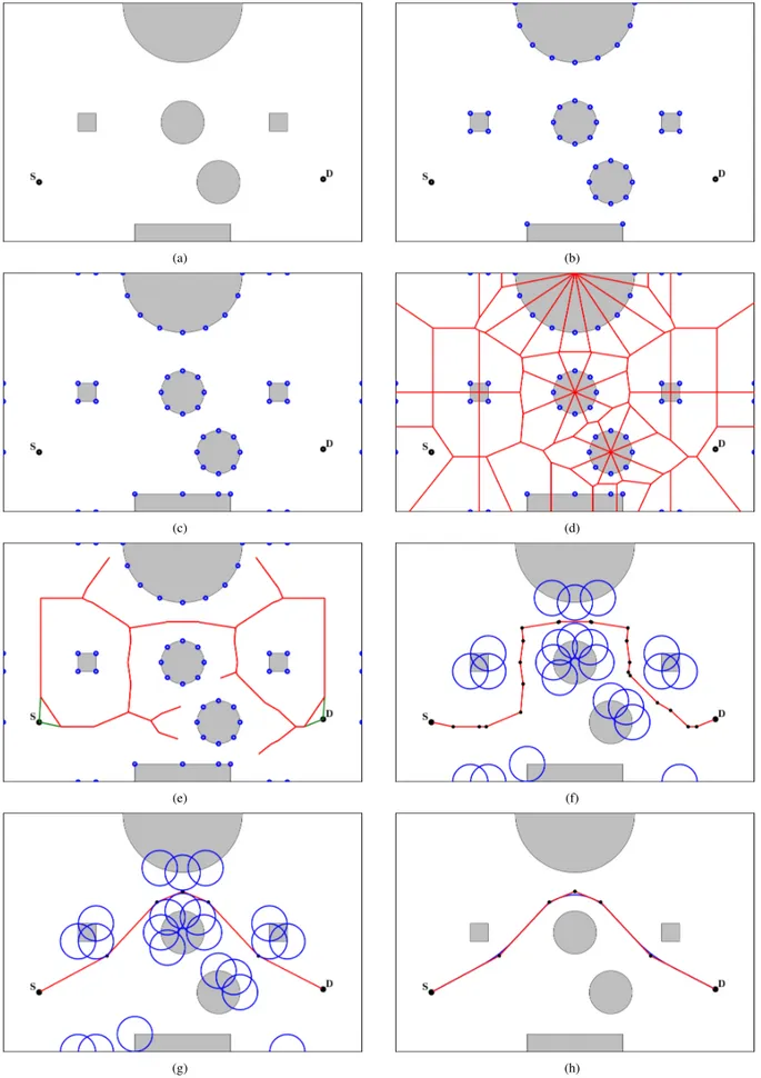
We illustrate the successive steps of our path planning method in Fig. 1, on a problem taken from the Eurobot case study. Fig. 1(a) shows the area with the obstacles, source point S and destination point D. Fig. 1(b) and Fig. 1(c) show how the obstacles and the borders of the area are approximated by finite set of points and their projections. Fig. 1(d) gives the Voronoi diagram of the considered set of points. Fig. 1(e) illustrates the insertion of source and destination points, as well as the deletion of the edges that conflict with obstacles. Fig. 1(f) shows the result of the A∗ shortest path search. The string-pulling operation is illustrated in Fig. 1(g), and the final result is shown in Fig. 1(h). The complete algorithm executes on a i5-460M processor running at 2.53GHz in less than 500µs. Fig. 1(h) also shows the interpolated path produced by [15], which is computed in milliseconds on the same processor.
IV. REFINEMENTS ANDFUTUREWORK
We now discuss some possible refinements and improve-ments of our path planning method.
A. Dealing with the Shape of the Robot
Robots are not always symmetrical, and can not generally be accurately represented by a single point. For a differential
drive robot, it is usually sufficient to consider the smallest disk that covers the robot, centered at the midpoint of the segment that links the two locomotion wheels. Our path planning method can be adapted to such robots by adding the radius of this disk to the required clearance. The generated path then corresponds to the one that will be followed by the center of the robot. Whatever the orientation taken by the robot along the path, it will never come closer to an obstacle than the imposed clearance.
It should be stressed out, however, that this approximation leads to a path planning strategy that may not be complete anymore, in the sense that some feasible paths may be missed. A long rectangular robot moving along its longer border could, for instance, be prevented from moving be-tween two close obstacles. This problem could be alleviated by employing a refined criterion for detecting the edges of the Voronoi diagram that need to be deleted. In the Eurobot case study, approximating robot shapes by disks turned out to be sufficient.
One can however carry out the string-pulling operation using a smaller clearance than for the path discovery step. Indeed, it is sufficient to only consider the largest distance between the center of the robot and its border, measured perpendicularly to its direction of travel. Intuitively, since the path that is considered already avoids obstacles by construction, and the direction of travel of the robot is tangent to this path, only lateral clearance of the robot with respect to the obstacles has to be ensured.
B. Imposing Initial and Final Orientation
We have defined the source S and destination D of a path as the locations initially and finally taken by the robot but, in most applications dealing with nonholonomic robots, one additionally needs to impose the orientation at that points. This can easily be achieved by constructing small line segments [SS0] and [D0D] that are traveled in the appropriate directions, and that will respectively be prepended and appended to a path computed from S0 to D0. The lengths of such segments must be consistent with the physical constraints imposed on the robot, for instance, a reasonable strategy is to make |SS0| at least equal to the braking distance of the robot at its initial speed. These segments must also clear obstacles. This approach has the advantage of generating paths with zero initial and final curvatures, which simplifies chaining successive paths.
C. Misled Searches
Using a Voronoi-based roadmap graph has many advan-tages, but since edges of Voronoi diagrams are located at the largest possible distance from obstacles, this approach has the drawback of distorting the length of paths. This can sometimes mislead the search algorithm, as the shortest path in the roadmap does not necessarily translate into the optimal one after performing the string-pulling operation.
This issue is illustrated in Fig. 2, which shows a problem instance for which our path planning algorithm generates a
(a) (b)
(c) (d)
(e) (f)
(g) (h)
Fig. 1. Illustration of the path planning method. (a) Problem statement. (b) Approximation of obstacles. (c) Projections added to borders. (d) Voronoi diagram. (e) Insertion of source and destination & edge deletion. (f) A∗search. (g) String pulling. (h) Smoothed solution.
(a) (b)
(c) (d)
Fig. 2. Issue with the Voronoi-based search. (a) Voronoi-based roadmap. (b) Shortest path in the roadmap. (c) Solution. (d) Overall shortest path.
path that is not optimal. This problem is especially noticeable when Cfree contains large zones that are free from obstacles.
We propose three solutions for dealing with this issue. First, one can insert in large empty zones of Cfree virtual
obstacles that provide additional sites for constructing the Voronoi diagram, but are not considered during the edge deletion step. Second, the shortest path search algorithm can be tuned by using an heuristic that reduces the weight of the edges that are far from obstacles, since such edges are likely to benefit the most from reductions by the string-pulling operation. This solution has the advantage of being easy to implement, but does not guarantee optimality. A third approach would be to integrate the string-pulling operation inside the search for the shortest path in the roadmap, which would produce an optimal solution. This last technique and its efficient implementation are still work in progress.
V. CONCLUSIONS
In this work, we have introduced an efficient path planning method for mobile robots. The computed path is made up of straight line segments, and can then be interpolated into a feasible trajectory for a differential drive or a tricycle robot, taking into account its physical constraints [15].
Strictly speaking, our algorithm is only complete for perfectly cylindrical robots, but this limitation is not an issue for the vast majority of applications, especially when robots are nearly symmetrical. The method does not provide a guarantee of optimality, but always produces paths that are reasonably short.
The algorithm needs O(n log n) total time, where n de-notes the number of points considered for approximating the obstacles. Indeed, the corresponding Voronoi diagram can be computed in O(n log n) time, and contains O(n) nodes. Inserting source and destination points, and deleting
conflicting edges, is then performed in O(n) time. The search for a shortest path in the roadmap is carried out in O(n log n) time, and produces a path with at most O(n) nodes. This path is then refined in O(n) time by the string-pulling procedure. The results presented in this paper have been successfully implemented in the robots built for Eurobot at the University of Li`ege since 2008, together with the path interpolation algorithm introduced in [15]. In this framework, the very low computational cost of this approach made it possible to perform near-optimal trajectory planning in real-time, which provided a clear competitive advantage.
REFERENCES
[1] F. Aurenhammer and R. Klein, “Voronoi diagrams,” Handbook of computational geometry, vol. 5, pp. 201–290, 2000.
[2] M. d. Berg, O. Cheong, M. v. Kreveld, and M. Overmars, Compu-tational Geometry: Algorithms and Applications, 3rd ed. Springer-Verlag TELOS, 2008.
[3] P. Bhattacharya and M. L. Gavrilova, “Roadmap-based path planning-using the Voronoi diagram for a clearance-based shortest path,” Robotics & Automation Magazine, IEEE, vol. 15, no. 2, pp. 58–66, 2008.
[4] S. Fortune, “A sweepline algorithm for Voronoi diagrams,” Algorith-mica, vol. 2, no. 1-4, pp. 153–174, 1987.
[5] R. Geraerts and M. H. Overmars, “A comparative study of proba-bilistic roadmap planners,” in Algorithmic Foundations of Robotics V. Springer, 2004, pp. 43–58.
[6] K. E. Hoff III, J. Keyser, M. Lin, D. Manocha, and T. Culver, “Fast computation of generalized Voronoi diagrams using graphics hardware,” in Proceedings of the 26th annual conference on Computer graphics and interactive techniques. ACM Press/Addison-Wesley Publishing Co., 1999, pp. 277–286.
[7] S. Kambhampati and L. S. Davis, “Multiresolution path planning for mobile robots,” DTIC Document, Tech. Rep., 1985.
[8] S. Karaman, M. R. Walter, A. Perez, E. Frazzoli, and S. Teller, “Any-time motion planning using the RRT*,” in Robotics and Automation (ICRA), 2011 IEEE International Conference on, 2011, pp. 1478– 1483.
[9] O. Khatib, “Real-time obstacle avoidance for manipulators and mobile robots,” The international journal of robotics research, vol. 5, no. 1, pp. 90–98, 1986.
[10] Y. Koren and J. Borenstein, “Potential field methods and their inherent limitations for mobile robot navigation,” in Robotics and Automation, 1991. Proceedings., 1991 IEEE International Conference on, 1991, pp. 1398–1404.
[11] J.-C. Latombe, Robot Motion Planning. Kluwer Academic Publishers, 1991.
[12] S. M. LaValle, Rapidly-Exploring Random Trees A New Tool for Path Planning. TR 98-11, Computer Science Department, Iowa State University, 1998.
[13] ——, Planning algorithms. Cambridge University Press, 2006. [14] D. T. Lee and F. P. Preparata, “Euclidean shortest paths in the presence
of rectilinear barriers,” Networks, vol. 14, no. 3, pp. 393–410, 1984. [15] S. Lens and B. Boigelot, “Efficient path interpolation and speed profile
computation for nonholonomic mobile robots,” 2015, submitted for publication.
[16] M. Pocchiola and G. Vegter, “Computing the visibility graph via pseudo-triangulations,” in Proceedings of the eleventh annual sym-posium on Computational geometry. ACM, 1995, pp. 248–257. [17] R. Wein, J. P. Van Den Berg, and D. Halperin, “The visibility–Voronoi
complex and its applications,” in Proceedings of the twenty-first annual symposium on Computational geometry. ACM, 2005, pp. 63–72.