HAL Id: hal-00749115
https://hal.archives-ouvertes.fr/hal-00749115
Submitted on 6 Nov 2012HAL is a multi-disciplinary open access archive for the deposit and dissemination of sci-entific research documents, whether they are pub-lished or not. The documents may come from teaching and research institutions in France or
L’archive ouverte pluridisciplinaire HAL, est destinée au dépôt et à la diffusion de documents scientifiques de niveau recherche, publiés ou non, émanant des établissements d’enseignement et de recherche français ou étrangers, des laboratoires
Implementation of Morphological Operators for Surface
Segmentation
Marcel Alcoverro
To cite this version:
Marcel Alcoverro. Implementation of Morphological Operators for Surface Segmentation. 2007. �hal-00749115�
Implementation of Morphological Operators for
Surface Segmentation
Marcel Alcoverro Vidal
Supervisor : Sylvie Philipp-Foliguet
Ecole Nationale Sup´erieure de l’Electronique et de ses Applications
Acknowledgements
Dedico aquest treball a la Lara, sense tu no hagu´es estat possible. Gr`acies per haver-me escoltat els rotllos dels watersheds i skeletons, per haver-haver-me animat en els mohaver-ments dif´ıcils. Tamb´e el vull dedicar als meus pares, que sou els qui heu aguantat tants maldecaps, tants anys. Ja s’ha acabat per fi la carrera infinita !
Je veux remercier Sylvie Phillipp, Michel Jordan, Laurent Najman et Jean Cousty pour m’accuellir dans leur ´equipes. Merci pour m’avoir d´ecouvert le monde de la recherche et me permettre participer de tr´es bonnes discussions. Merci Jean pour consacrer ton temps `a m’aider a ne me perdre pas dans les chemins de la morphologie.
Resum
Aquest treball forma part del projecte Eros3d, el qual tracta la gesti´o de bases de dades d’obres d’art. El C2RMF (Centre de Recherche et de Restauration des Musees de France) ha organitzat durant uns anys les tasques de digitalitzaci´o dels museus francesos i actual-ment es disposa d’una base de dades de 650 objectes 3D. El seu objectiu ´es dissenyar una arquitectura de software capa¸c d’emmagatzemar i manejar (visualitzar, cercar, comparar) les dades per diferents nivells d’usuari. Concretament el treball realitzat forma part d’un sistema de recuperaci´o de dades segons el contingut.
Un sistema de recuperaci´o de dades segons el contingut (content-based retrieval system) recupera els objectes de la base de dades basant-se en la similaritat entre els objectes. La base de dades ha d’indexar-se per tal de dur a terme la classificaci´o i cerca, i per realitzar la indexaci´o s’utilitzen vectors de caracter´ıstiques per a cada objecte. El plantejament adoptat per a l’obtenci´o de les caracter´ıstiques de cada objecte ´es la segmentaci´o de la superf´ıcie del model en diferents regions significatives. Posteriorment es realitza un c`alcul de diferents trets caracter´ıstics per a cada regi´o. Aquestes diferents caracter´ıstiques obtingudes per a cada model 3D serviran tant per a comparacions basades en l’objecte sencer, com tamb´e per realitzar consultes parcials consistents en la cerca a partir d’un conjunt de regions de la superf´ıcie de l’objecte.
La divisi´o de la superf´ıcie de l’objecte es realitza partint d’un mapa de curvatura calculat sobre la malla triangular que representa l’objecte. L’operador utilitzat per fer la partici´o ´es la transformada watershed (l´ınia divis`oria d’aig¨ues) aplicada sobre el mapa de curvatura. El watershed ´es un operador morfol`ogic molt utilitzat en el processament d’imatge. Si imaginem una funci´o com un relleu topogr`afic on els valors de cada punt s´on l’al¸cada d’aquest punt en el relleu, un regi´o seria el conjunt de punts on si i caigu´es una gota d’aigua, aquesta baixaria fins al fons d’una mateixa vall. Partint d’una funci´o en un espai determinat, el watershed obt´e regions que extenen els m´ınims regionals de la funci´o. En el nostre cas, representem la funci´o curvatura sobre la malla 3D amb un graf valuat en les seves arestes. Apliquem la transformada watershed sobre aquest graf utilitzant l’algorisme presentat per Jean Cousty [5] de c`alcul de watersheds en grafs valuats en les arestes.
La transformada watershed aplicada sobre una funci´o obt´e un nombre de regions equi-valent al nombre de m´ınims regionals de la funci´o de partida. El resultat ens pot portar a una sobre-segmentaci´o no desitjada. Per tal de controlar el nombre de regions obtingudes pel watershed aix´ı com les caracter´ıstiques d’aquestes regions, abans del c`alcul d’aquest, filtrem la funci´o original per tal de reduir-ne el nombre de m´ınims regionals. L’operador que implementem per al filtratge de la funci´o de curvatura original ´es l’arbre de
compo-nents. La combinaci´o arbre de components + watershed ha estat ampliament utilitzada en
processat d’imatge, v´ıdeo i senyal, i aporta robustesa als resultats de segmentaci´o obtinguts amb el watershed. L’algorisme implementat ´es una adaptaci´o original de l’algorisme per al c`alcul de l’arbre de components presentat per Najman i Couprie [14].
L’arbre de components ´es un estructura que ordena els components connexos d’un graf. Considerem un graf valuat G. Un component connex d’aquest graf G ´es un subgraf de G connex en que els seus nodes o arestes tenen el mateix valor. L’arbre de
compo-nents estableix una jerarquia entre els diferents compocompo-nents connexos d’un graf. Aleshores mitjan¸cant aquest arbre podem modificar els valors del graf de manera que eliminem els components connexos que no desitgem. En el nostre cas els valors del graf son els valors de curvatura de la superf´ıcie de l’objecte que analitzem. Si per exemple considerem un component connex petit de valor molt petit, aquest correspondr`a a una zona de la su-perf´ıcie de l’objecte petita amb molta curvatura. Aquesta zona pot correspondre a una irregularitat poc significativa de la superf´ıcie, o a sorolls en el proc´es d’obtenci´o del model. Mitjan¸cant l’arbre de components els valors de curvatura d’aquesta zona prendran els va-lors dels punts adjacents, de manera que la irregularitat de la funci curvatura desapareix. Mentre la transformada watershed obtindria una regi´o per aquesta zona petita del mapa de curvatura original, al aplicar-la al mapa filtrat per l’arbre de components aquesta zona no significativa ja no apareix.
Un cop obtingudes les diferents regions de la superf´ıcie es calculen tres caracter´ıstiques diferents per cada regi´o. Per una banda un histograma de la longitud de les cordes (dist`ancia d’un punt al baricentre) i angle amb els eixos principals de l’objecte. Un altre s un histograma de valors de curvatura. Per ´ultim, l’histograma EGI (Extended
Gaus-sian Images). Considerem una esfera de Gauss de l’objecte, l’histograma EGI compta les
projeccions de cada punt de l’objecte en aquesta esfera. En el nostre cas el recompte es realitza per cada regi´o.
A partir dels histogrames de cada regi´o es poden construir els vectors de caracter´ıstiques necessaris per la indexaci´o de la base de dades d’objectes. El m`etode presenta avantatges respecte t`ecniques d’extracci´o de caracter´ıstiques geom`etriques globals ja que permet trobar similaritats i difer`encies en objectes que tenen la mateixa forma i on els trets caracter´ıstics es troben en detalls de la superf´ıcie. Aquest ´es el cas per exemple de les escultures antigues que trobem a la base Eros3d provinents del Museu del Louvre, on la forma d’aquestes ´es pr`acticament cil´ındrica, mentre que les particularitats es troben esculpides sobre la superf´ıcie.
Abstract
A content-based retrieval system needs feature vectors for database indexation. We adopt the surface segmentation approach to obtain several features for a 3D object which can be used to retrieve objects in a database from a partial request composed from a set of regions. To achieve the segmentation of the surface into several regions we apply the watershed transform on a curvature map computed on the 3D surface mesh. The watershed applied directly on the original curvature map produces an over-segmentation of the object surface. Thus, we previously filter the original curvature map by using the component tree. After this filtering, the watershed transform is computed on the filtered curvature map and we obtain the desired number of regions. Then we proceed by computing some features for each region obtained, which will serve as feature vectors for a content-based search and retrieval system. The techniques we apply on the surface of 3D objects have been presented for image applications.
Consider a 3D triangular mesh (a set of points, triangles and sides of triangles). We build an edge weighted graph to represent the mesh. Weights on edges of the graph corre-spond to the curvature map computed on the mesh. The component tree is a structure to order the connected components of a weighted graph. We implement an original algorithm to build the component tree of an edge weighted graph based on the one presented by Najman and Couprie [14]. This structure allows to reduce the number of minima of the original map on edges of the graph. We implement the algorithm proposed by Cousty [5] to compute the watershed transform on an edge weighted graph. By using the watershed transform we obtain a number of regions of the map which equals the number of minima of the input map.
Once we obtain the partition of the mesh into several regions we compute features of each region. These features consist in histograms for each region considering three differ-ent approaches: Extended Gaussian Images (EGI) [8]; a cords histogram (considering the cords lenght and a principal angle); a curvature histogram (considering principal curva-tures). These histograms form feature vectors for each region which will help the database indexation and classification.
Contents
1 Introduction 7
2 Mesh characterization and surface analysis 7
2.1 Edge-weighted graphs . . . 8
2.2 Simplicial complexes . . . 9
2.3 Curvature . . . 10
2.4 Vertex per-face graph . . . 12
2.5 Mesh Repair . . . 12
3 Watershed 14 3.1 Extensions and graph cuts . . . 15
3.2 Watersheds and catchment basins . . . 15
3.3 Minimum spanning forests and watershed optimality . . . 17
3.3.1 Minimum spanning forests and minimum spanning trees . . . 18
3.4 Watershed algorithm . . . 19
3.5 Border thinning on simplicial complexes . . . 21
4 Component tree 23 4.1 Connected components notions . . . 24
4.2 Component tree definition . . . 25
4.3 Component tree and minimum spanning tree . . . 25
4.4 The Union-Find method . . . 27
4.5 Component tree algorithm . . . 28
4.5.1 High-level view . . . 28 4.5.2 Detailed view . . . 29 4.5.3 Example . . . 32 4.6 Node Attributes . . . 35 4.7 Filtering . . . 37 5 Region attributes 38 5.1 Cords histogram . . . 38
5.2 Extended Gaussian Images . . . 39
5.3 Curvature histogram . . . 40
6 Experimental results 40
1
Introduction
The recent development of 3D object acquisition methods involve a need to handle this kind of information. Nowadays 3D object databases appear in various areas for leisure as well as for scientific applications (medical, industrial part catalogues, cultural heritage, etc.). Large database can be quickly populated using 3D mesh acquisition and reconstruction tools which have become easy to use. As database size is growing, tools to retrieve infor-mation as indexing methods, search algorithms and data classification techniques become more and more important.
A significant amount of work has been done in the past two decades on text-based document retrieval. The Google search engine has become a standard as text-based search engine. Indexing by keywords and search achieved through text retrieval techniques has the advantage that it is “high level” (semantic level), but keywords are external information which is often manually assigned. More recently content-based retrieval systems have been developed for images, audio, and video to automatically index and retrieve information from digital libraries. Content-based retrieval systems retrieve objects based on the integral similarity of objects.
In search-by-similarity, the goal is to find objects which are “close” to the example. It is done with respect to a given similarity measurement and thanks to object indexes computed on object features. These features may be of various kinds (points, segments, regions, etc.) and may have different properties such as scale invariance, rotation invariance, etc.
Different techniques can be used to extract features of the 3D object, that can be obtained from a shape representation (Global feature-based techniques, graph-based tech-niques, recognition-based techniques). Surface segmentation can be applied also for feature detection.
This work is part of the Eros3d project. The Eros3d project deals with artwork database management. C2RMF (Centre de Recherche et de Restauration des Musees de France) has organized digitalization lobbying in french museums for some years. 650 3D objects are available in the database. Its aim is to design a software architecture that is supposed to store and handle (view, research, compare) data at different user levels.
2
Mesh characterization and surface analysis
Segmentation of a polygonal mesh is a method of splitting the mesh into regions in a “meaningful” manner. A mesh consists of a set of n points (xi ∈ E3; 0≤ i < n) and a set
of planar convex polygons made up of these points. A first question to consider in order to partition the mesh is to define which components of the mesh will form the regions and how their boundaries will be defined. Two different approaches that have been used before are summarized in [17], called vertex based method and edge based method.
The vertex based methods consider a value associated at each vertex (i.e curvature) and define the segmentation as regions that consist of connected vertices that have the same property. A major drawback in this approach is that no boundaries are created
for the regions and each vertex has its own region information. Therefore triangles have multi-region information, so the three vertices of a triangle can be part of three different regions, whereas the triangle itself would not belong to any region.
The edge based methods define an edge as boundary if it is shared by two planes whose normal vectors make an angle greater than a certain threshold. This results in disconnected boundary edges and thereby open regions.
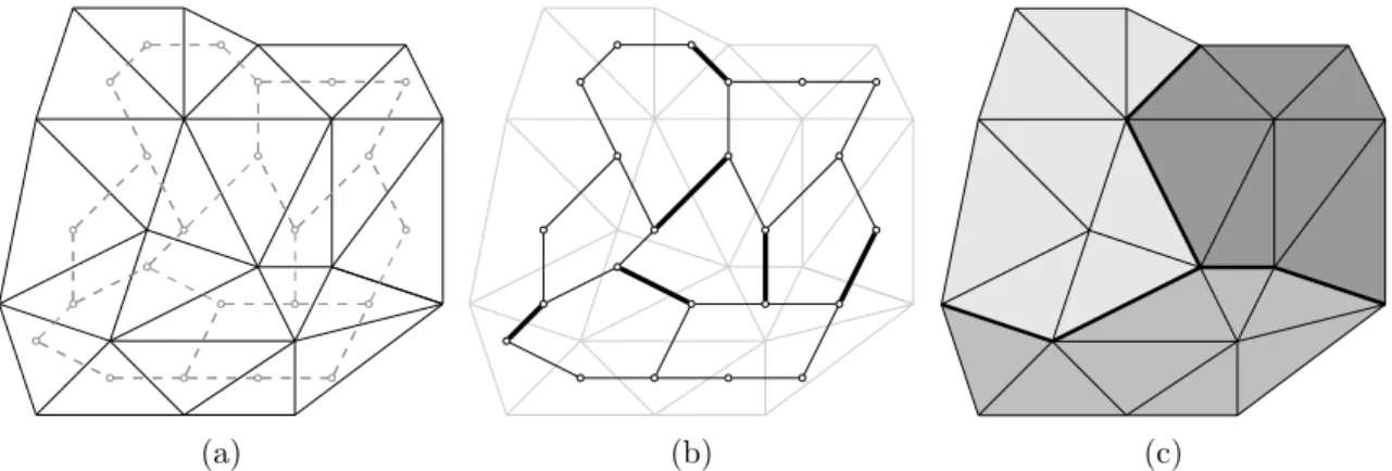
Our approach defines regions as sets of connected faces with edges as their boundaries, that leads to obtain a surface divided in closed independent regions consisting of connected triangles after the segmentation process. We illustrate our approach in fig. 3.
We represent the mesh by a graph, and the curvature will we defined as a weight function on edges, so we will introduce some notations for edge-weighted graphs. Also we will introduce some notions on simplicial complexes, since it is a structure that allows to describe the topological properties of a mesh.
2.1
Edge-weighted graphs
We define a graph as a pair X = (V (X), E(X)) where V (X) is a finite set and E(X) is composed of unordered pairs of V (X),i.e, E(X) is a subset of {{x, y}⊆ V2(X) | x$= y}.
Each element of V (X) is called a vertex and each element of E(X) is called an edge. Let X be a graph. Let x and y be vertices of X. We say that x and y are adjacent if {x, y} is an edge of X. A sequence π =%x0, . . . , xl& of vertices of X is a path in X (from
x0 to x1) if xi and xi+1 are adjacent for each i = 0, . . . , l− 1. We say that X is connected
if, for any pair of vertices (x, y) in X, there is a path in X from x to y.
Let X and Y be two graphs. If V (Y ) ⊆ V (X) and E(Y ) ⊆ E(X), we say that Y is
a subgraph of X and we write Y ⊆ X.
Let X and Y be two graphs and Y ⊆ X, Y a subgraph of X. We say that Y is a
connected component of X, or simply a component of X, if Y is a connected subgraph of
X which is maximal for this property, i.e, for any connected graph Z, Y ⊆ Z ⊆ X implies Z = Y .
Throughout this paper G denotes a connected graph.
We denote by F the set of all maps from E to R. Let F ∈ F. If u is an edge of G, F (u) is the altitude of u. In our application the curvature will define the altitude of the edges of the graph. We also will denote by F the map from V to R such that for any x∈ V , F (x) is the minimal altitude of an edge at x, i.e., F (x) = min{F (u) | u ∈ E, x ∈ u} Let X ⊆ G and k ∈ R. A subgraph X of G is a minimum of F (at altitude k) if:
- X is connected;
- the altitude of any edge adjacent to X is strictly greater than k.
We denote by M(F ) the graph whose edge set is the union of the edge sets of all minima of F .
2.2
Simplicial complexes
We extract from [2] and [3] some notions and notations of complexes.
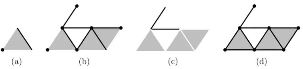
A (finite simplicial) complex X is a finite family composed of finite nonempty sets such that, if f is an element of X, then every nonempty subset of f is an element of X. Each element of a complex is called face. The dimension of a face f is the number of its elements minus one. We call an m-face a face of dimension m. We denote by K the collection of all complexes.
In fig. 1(a) we ilustrate a graphical representation of a 0-face, a 1-face and a 2-face.
(a) (b) (c) (d)
Figure 1: (a) A set of faces (one 2-face, one 1-face, one 0-face). (b) A set of faces X which is not a complex. (c) The set X+, all the facets of X. (d) The set X−
, the closure of X, which is a complex.
Let f be a finite nonempty set. We set ˆf = {g|g ⊆ f, g $= ∅} and ˆf∗
= ˆf \ {f }. Any g ∈ ˆf is a face of f , and any g ∈ ˆf∗
is a proper face of f. If X is a finite set of faces in Fn
2, we write X −
=∪{ ˆf |f ∈ X}, X−
is the closure os X. Thus, a finite family X of finite nonempty sets is a complex if and only if X = X−
.
Any subset Y of a complex X which is also a complex is a subcomplex of X, and we write Y * X. If X is a complex in K we also denote X * K.
Let X * K. A face f ∈ X is a facet of X if there is no g ∈ Y such that f ∈ ˆg∗
. We denote by X+ the set composed of all facets.
In fig. 1 we ilustrate these notions. The set of faces X of fig. 1(b) are not a complex. As it can be observed, X does not equal its closure X−
2.3
Curvature
The computation of the curvature has been done with the software Trimesh provided by Princeton University [18]. This software provides a method based on computing first the curvature per-face and then estimates the value at each vertex as a weighted average over the immediately adjacent faces.
The normal curvature κn of a surface in some direction is the reciprocal of the radius
of the circle that best approximates a normal slice of surface in that direction. The normal curvature can be expressed as κn= κ1s2+κ2t2 where κ1and κ2 are the principal curvatures
and (s, t) are the principal directions, which are the directions where the normal curvature reaches its minimum and maximum. These directions are ortogonal.
The Gaussian curvature K is equal to the product of the principal curvatures: K = κ1κ2, and the mean curvature H is their average: H = (κ1+ κ2)/2.
(a) (b) H (c) K
(d) D (e) Hinv (f) M
Figure 2: Curvature scalar functions of the object in (a) in grayscale.
κ2 on each vertex of the mesh. These values increase with the convexity of the surface.
They decrease into negative values on concave zones , getting low absolute values on flat zones. Considering the combination of the principal curvatures κ1 and κ2 on a surface we
have convex zones when both values are great positive, concave zones when both are great negative and saddle zones when one value is great positive and the other great negative, meaning convexity in one direction and concavity in the other. The flat zones have both values low.
As the curvature map will be used to partition the surface by using the watershed operator, a single scalar function is desired. Several approaches can be done to obtain this height function by combining values κ1 and κ2. Mainly, the choice will depend on the
desired further applications. Also the class of objects or their shape characteristics may determine which are the “meaningful” regions. For example, if we are dealing with objects made of flat smooth poligonal parts (cars, manufactured pieces, furniture, etc.), we should be interested in obtaining regions of this flat parts, thus the divide line between regions would be placed on high curvature edges. In the case of art objects, the pieces could be characterized by their carved features, thus it would be interesting to place the lines on the concave zones dividing convex parts.
Mangan and Whitaker [11] use as magnitude for curvature the deviation from flatness D =√4H2− 2K2
where H is the mean curvature and K the gaussian curvature. This function gives high values on convex and concave zones, while it is low on flat and saddle zones.
Other approach we adopted is to use mean curvature H in the form Hinv = arctan (−H + π/2)
This function has the behavior of the inverse of the mean curvature, but taking always positive values. It gives high values to concave zones and low values to convex zones.
We consider also a max curvature as
M = max(κ21, κ22)
and that gives high values on convex and concave zones, as H2. The max curvature has
also high values on zones that are flat in one direction, and convex or concave in the other. This zones are commonly the edges that divide planes of an object, as the division between the roof and the doors of a car.
We have used this different treatments of the principal curvatures and, for the art objects we deal with, the Hinv function is the one with which we obtained the best results,
while the max curvature M gives better results for manufactured objects.
In fig. 2 are depicted the values of these scalar functions in grayscale for the sculpture in fig. 2(a). Low values are black, while great values are white.
(a) (b) (c)
Figure 3: (a) A triangle mesh and a vertex per-face graph. (b) Segmentation on edges of the graph (in bold). (c) Segmentation on the mesh.
2.4
Vertex per-face graph
Consider a 3D surface mesh M (composed of points,triangles, sides of the triangles) so that for any side e in M there is exactly one pair of triangles (g, h) such that e ∈ g and e ∈ h. We build a graph G = (V, E, F ) with one vertex for each face of M and an edge connecting two vertices if the corresponding two faces share a side. We will call this graph
a vertex per-face graph. An example of a vertex per-face graph is depicted in fig. 3(a).
Let be e any side of a triangle in M and (x, y) the pair of points such that e = {x, y}. As described in section 2.3 we have computed the curvature values in each point of the mesh. We denote them as κ1x, κ2x and κ1y, κ2y for the points x and y respectively. Then
we will compute for each e in M, κ1 =
κ1x+ κ1y
2 κ2 =
κ2x+ κ2y
2
Considering then the scalar curvature functions explained above (section 2.3) we obtain then a map from E into R that we denote by F , that will represent the curvature between each two adjacent faces of the mesh.
2.5
Mesh Repair
The triangle meshes obtained from acquisition of real-objects and also CAD generated models often have defects that may cause problems in further processing. In our case the condition that will allow us to proceed properly would be a triangular surface mesh that forms a manifold without boundaries. Thus, the set of points, edges and triangles that form a mesh should be a complex K, in which ∀ 1-face u ∈ K there exists exactly two 2-faces f ∈ K, g ∈ K, such that f ∩ g = u. If this is acomplished we can obtain the vertex per-face graph described previously.
The degeneracies that usually appear may be holes, tubes, duplicated faces, intersecting faces or borders, and not all of them can be solved in the same way. We have tried different
approaches, which have been based on available software, as it was out of our scope to implement a new application for mesh repairing purposes.
The application ReMESH [1] provides an interactive environment for repairing meshes. A visualization tool is provided, and the software allows to detect several degeneracies, as duplicated faces, holes, intersecting triangles. It provides also tools to remove the defects, to fill holes after, and also has utilities to build again the mesh. We have not used this application for repairing our objects, as with it meshes should be repaired manually, and for our purposes the approach should be automatic. Even though, it has been useful to visualize the kind of degeneracies we deal with, to plan other approaches and to test if the other approaches worked well.
In order to get the proper meshes, we use two different automatic approaches. Both of them rebuild the mesh as it assures that the definitive mesh acomplishes our conditions. Also for both of them the steps involved have been the same, voxelization, isosurface
extrac-tion, mesh smoothing and mesh size optimization similar as it is presented by Nooruddin
and Turk [15] . The differences are on the techniques adopted on the voxelization step. Voxelization Voxelization means converting a polygonal model into a volume. The first approach used to reach the volume from the original mesh has been using the library Pink [4] to proceed with the following steps:
- obtain the points (i.e vertices of each triangle) of the mesh, and build a 3D grid where we place the points.
- calculate a distance map of this grid. Each cell of the grid get a value which is the minimum distance to a point, while point cells get 0 value.
- apply a watershed segmentation on the inverse of the distance map. We use markers for the watershed that are: a point in the interior of the object; a frame of the grid as marker for the exterior.
The watershed operator produces a divison of the grid into two regions, that are the interior and the exterior of the object. We found problems in this approach due to the need for automatisation. One problem comes from obtaining a point of the interior of the object as marker for the watershed. A implementation of a method in a step before the extraction of the vertices of the mesh into the grid is needed. We used the barycenter of the object as marker, but it fails as it is not always in the interior. Other problem is that the resulting volume may have broken parts corresponding to thin parts of the original mesh.
The other approach we tested for the voxelization is the one presented at [15], which has been implemented at Princeton [13]. The method used is called parity count which consists in classify a voxel V by counting the number of times that a ray with its origin at the center of V intersects polygons of the model. An odd number of intersections means that V is interior to the model and even number means that it is outside. To improve the technique for models that have cracks or holes, that will cause a bad classification, a voting scheme is adopted, by using more directions for the rays, and classifying by a
majority vote. This approach worked well, even though it creates some tunnels due to degeneracies not solved by the voting scheme. At [15] is proposed to apply morphological operators to fill this tunnels, as erosion and dilation, but it has not been tested.
Isosurface extraction After the voxelization step we extract an isosurface from the volumetric representation to create a manifold polygonal model. We used the library Pink for this computing, which implements a topologically correct Marching Cubes algorithm [10].
Mesh smoothing The isosurfaces extracted after the marching cubes algorithm result in a staircase surface. We use Taubin’s smoothing technique implemented in Trimesh [18] wich creates a new surface smoother than the original by using a low-pass filter over the position of the vertices.
Mesh size optimization The surface mesh produced by the marching cubes algorithm is usually over-tessellated. We used the software Yams [6] to optimize the triangle count of the mesh. The remeshing algorithm produce a mesh where elements size is related to local curvature.
After these steps we obtain a new mesh free of degeneracies that acomplishes our conditions of a maniflod without boundaries. Even though, the method should be improved to perform better in some cases, as when it generates tunnels in the resulting object, or broken thin parts. Also the automatisation of resolution related parameters should be improved.
3
Watershed
The watershed transform has been widely used as a fundamental step in many segmenta-tion procedures. This algorithm operates on a height funcsegmenta-tion which is defined over the corresponding domain. It was introduced for image segmentation and also has been used on 3D surfaces [11]. We use the algorithm introduced by Cousty [5] which is defined on the framework of edge-weighted graphs.
The watershed method derives the name from the manner how it segments its height function domain in catchment basins. Imagine a drop of water falling on a relief described by the height function. It will follow the steepest descent path until it reaches a local minimum. The set of points whose steepest descent paths terminate at the same minimum of the function forms a catchment basin. The watershed line will be the line that separates the different catchment basins.
In our case the height function F is the curvature defined on the edges of a graph G = (V, E, F ) and the regions of the watershed are computed as a extension of the minima of that graph.
3.1
Extensions and graph cuts
The notions of extension and graph cut are important to define the method used to compute the watershed. The following definitions are extracted from [5] and formalize both notions for the framework of graphs.
Definition 1. Let X and Y be two non empty subgraphs of G. We say that Y is an
extension of X (in G) if X ⊆ Y and if any component of Y contains exactly one component
of X.
The subgraphs drawn in bold in Fig.4(b) and Fig.4(c) are extensions of the subgraph in Fig.4(a).
Producing an extension until it covers all the vertices of the graph will form a separation that is called a graph cut.
Definition 2. Let X ⊆ G and S ⊆ E. We say that S is a (graph) cut for X if S is an
extension of X and if S is minimal for this property, i.e., T ⊆ S and T is an extension of X imply T = S.
The set S depicted in Fig.4(d) is a cut for the subgraph X in Fig.4(a). S in Fig.4(c) is an extension of X, and it can be seen that it is a maximal extension.
(a) (b) (c) (d)
Figure 4: A graph G where in bold there is: (a) a subgraph X of G. (b) an extension of X. (c) an extension Y of X which is maximal. (d) a cut S for X such that S = Y .
3.2
Watersheds and catchment basins
The notion of a watershed can be defined by its catchment basins or by the properties of the divide line. Usually the first approach is used on a vertex-weighted graph framework, and the catchment basin of a minimum M is defined as the points from which M is reached by a steepest descent path. Following this definition, several catchment basins may overlap each other, as some points could have a steepest descent path to different minimas. To avoid this situation, some autors define the catchment basins as the points from which only a unique minimum is reached by a path with steepest descent, but in this latter definition some sets of points appear not belonging to any catchment basin.
From the notions of extension and graph cut we will introduce the watershed cut, as the “lines” that separate catchment basins, and their properties will be formalized by the drop of water principle. Later we will show that the watershed can be defined by the divide lines or the catchment basins. The following definitions are extracted from [5].
Let π =%x0, . . . , xl& be a path in G. Path π is descending (for F) if, for any i ∈ [1, l−1],
F ({xi−1, xi})≥ F ({xi, xi+1}).
Definition 3 (drop of water principle). Let S ⊆ E. We say that S satisfies the drop of water principle (for F ) if S is an extension of M(F ) and if for any u = {x0, y0}∈ S,
there exist π1 = %x0, . . . , xn& and π2 = %y0, . . . , ym& which are two descending paths in S
such that:
- xn and ym are vertices of two distinct minima of F ; and
- F (u)≥ F ({x0, x1}) (resp. F (u)≥ F ({y0, y1})), whenever π1 (resp. π2) is not trivial.
If S satisfies the drop of water principle, we say that S is a watershed cut, or simply a
watershed of F .
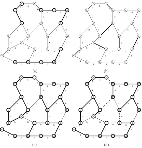
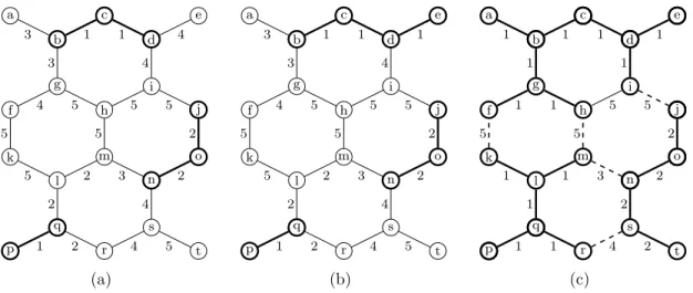
We will illustrate the previous definition with the graph G and the map F depicted in Fig. 5. In Fig. 5(a) it can be observed the set that composes the minima M(F ) (in bold). Consider the set of edges S at Fig. 5(b). It can be seen that S (Fig. 5(c)) is an extension of M(F ). Let s0 = {e, f } ∈ S the edge at altitude 6 at the corner bottom left of the graph
G. There exists a descending path π1 =%f, k, o& with o a vertex of the minima at altitude
1. Also there is the path π2 =%e, a& with a a vertex of a different minima at altitude 3. The
first edge of π1 (resp.π2) is lower than s0, F (s0) > F ({f, k}) (resp. F (s0) > F ({e, a})). As
this properties can be verified for each edge in S, S satisfies the drop of water principle. Thus S is a watershed cut of F .
In the framework of edge-weighted graph, we define a catchment basin as a component of the complementary of a watershed. In the following we will show that the watershed can be defined equivalently by the catchment basins or by the divide lines. We will introduce the notion of a path with steepest descent in order to later establish the consistency of the watershed cuts.
From now on, we also denote by F the map from V to R such that for any x∈ V , F (x) is the minimal altitude of an edge which contains x.
Let π = %x0, . . . , xl& be a path in G. The path π is a path with steepest descent for F
if, for any i∈ [1, l], F ({xi−1, xi}) = F (xi−1).
Definition 4 (steepest descent). Let S ⊆ E be a cut for M(S). We say that S is a basin cut of F if, from each point of V to M(F ), there exists, in the graph induced by S,
a path with steepest descent for F .
Theorem 1 (consistency). Let S ⊆ E. The set S is a basin cut of F if and only if S is
a watershed cut of F .
Consider the three components of the set depicted in bold in Fig. 5(c). It can be seen that there is a path with steepest descent from each vertex V to the minima, thus these
a b c d e f g h i j k l m n o p q r s t u v w 4 3 3 3 5 6 7 5 5 6 4 4 6 5 3 4 5 6 7 2 3 7 6 5 6 1 5 4 1 (a) a b c d e f g h i j k l m n o p q r s t u v w 4 3 3 3 5 6 7 5 5 6 4 4 6 5 3 4 5 6 7 2 3 7 6 5 6 1 5 4 1 (b) a b c d e f g h i j k l m n o p q r s t u v w 4 3 3 3 5 6 7 5 5 6 4 4 6 5 3 4 5 6 7 2 3 7 6 5 6 1 5 4 1 (c) a b c d e f g h i j k l m n o p q r s t u v w 4 3 3 3 5 7 5 5 4 4 5 3 4 5 2 3 6 5 6 1 5 4 1 6 6 6 6 7 7 (d)
Figure 5: A graph G and a map F where in bold there is. (a) The minima M (F ). (b) S a watershed cut of F . (c) An extension of M (F ) which is also S. (d) A MSF relative to M (F ) where dashed edges represent the induced cut.
components are the catchment basins (regions) and its complementary (Fig. 5(b)) the basin cut.
3.3
Minimum spanning forests and watershed optimality
We will introduce the notion of minimum spanning forests. From this notion we will derive in next sections the algorithm for the watershed computation. Also, as we will see, as minimum spanning forests of the minima of a map induce the watershed of the map, we will be able to state an optimality of the watershed cuts.
X if:
i) Y is an extension of X; and
ii) for any extension Z ⊆ Y of X, we have Z = Y whenever V (Z) = V (Y ).
We say that Y is a spanning forest relative to X (for G) if Y is a forest relative to X and V (Y ) = V .
Usually the notion of forest is defined as a graph which does not contain any cycle. Let X a subgraph of G, the weight of X (for F ) is the value F (X) =!
u∈E(X)F (u).
Definition 5. Let X and Y be two subgraphs of G. We say that Y is a minimum spanning forest (MSF) relative to X (for F , in G) if Y is a spanning forest relative to X and if the
weight of Y is less than or equal to the weight of any other spanning forest relative to X. In this case, we also say that Y is a relative MSF.
The minimum spanning forest (MSF) relative to the minima (depicted in bold in fig. 5(a)) is depicted in bold in the graph G of fig. 5(d).
The following statement will help to intuitively establish later the optimality of water-sheds.
Let X be a spanning forest relative to M(F ). The graph X is a MSF relative to M(F ) if and only if, for any x in V , there exists a path in X from x to M(F ) which is a path with steepest descent for F .
Let X be a subgraph of G and let Y be a spanning forest relative to X. There exists a unique cut S for Y and this cut is also a cut for X. We say that this unique cut is the
cut induced by Y . Furthermore, if Y is a MSF relative to X, we say that S is a MSF cut for X.
Theorem 2 (optimality). Let S ⊆ E. The set S is a MSF cut for M(F ) if and only if S is a watershed cut of F .
In fig. 5(d) dashed edges represent the cut induced by the MSF, which is also the watershed of G (fig.5(b)).
3.3.1 Minimum spanning forests and minimum spanning trees
A tree is usually defined [21] as a connected graph with no circuits, and a spanning tree of a connected graph G is a tree in G which contains all nodes of G. If we define the weight of a tree as the sum of the weights of its constituent edges, the minimum spanning tree of a graph G is a spanning tree whose weight is minimum among all spanning trees of G.
We can derive a definition of the tree from the notion of forest.
Let X ⊆ G. We say that X is a tree (resp. spanning tree) if X is a forest (resp. spanning forest) relative to the subgraph ({x},∅), x being any vertex of X.
Let X ⊆ G. The graph X is a minimum spanning tree (for F , in G if X is a MSF relative to the subgraph ({x},∅), x being any vertex of X.
We will present a construction that allows to give an equivalence of finding the minimum spanning tree and finding a MSF rooted on any subgraph X of G.
Let us consider first a subgraph X ⊆ G composed of isolated vertices. Let us construct a new graph G′
= (V′
, E′
) which contains an additional vertex z /∈ V linked by an edge to each vertex of X, thus V′ = V
∪ {z} and E′ = E
∪ Ez, where Ez = {{x, z}|x ∈ V (X)}.
Let us consider the map F′
from E′
to R such that, for any u ∈ E, F′
(u) = F (u), while for any u∈ Ez, F′(u) = kmin− 1, where kmin is the minimum value of F .
Let Y be any subgraph of G and let Y′ be the graph such that V (Y′) = V (Y )
∪ {z} and E(Y′
) = E(Y )∪ Ez. It may be seen that Y′ is a minimum spanning tree for F′ in G′ if
and only if Y is a MSF relative to X for F in G.
Following this construction we can extend it to the case of X being any subgraph of G. In this case, first we will contract each component of X into a single vertex, and if two vertices of this resulting graph must be linked by more than one edge we will keep only the one with minimal value. After we will proceed with the construction explained above. The minimum spanning tree computational construction has been widely studied. Con-sidering this construction the relative MSF can be computed using any minimum spanning tree algorithm.
3.4
Watershed algorithm
In order to introduce the method used to compute the watershed we will define first an edge classification based on local properties. Then we will also define the lowering operation and the thinning that will let us understand the strategy used to compute the watershed.
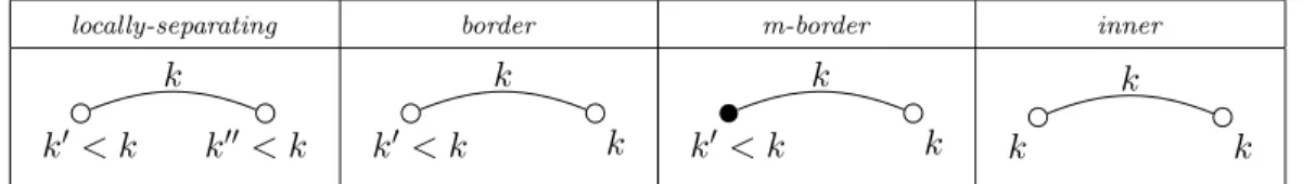
As we said before if x is a vertex of G, F (x) is the minimal altitude of an edge at x. Definition 6. Let u = {x, y}∈ E.
We say that u is locally separating (for F ) if (F (u) > max(F (x), F (y)).
We say that u is border (for F ) if (F (u) = max(F (x), F (y)) and (F (u) > min(F (x), F (y)). We say that u is minimum-border (for F ), written M-border if u is border and if exactly one of the vertices in u is a vertex of M(F ).
We say that u is inner (for F ) if F (x) = F (y) = F (u).
Fig. 6 illustrates this classification. In fig. 5(a) edges {k, f } or {l, g} are examples of border edges, {e, f } or {m, i} are locally-separating, {k, o} or {q, n} are m-border, and {a, b} or {w, q} are examples of inner edges.
locally-separating border m-border inner
k k′ < k k′′< k k k′ < k k k k′ < k k k k k
Figure 6: Edge classification in a weighted graph. In the m-border case the black vertex means that belongs to a minimum.
Definition 7. Let u ∈ E. The lowering of F at u is the map in F, denoted by [F \ u],
such that:
-[F \ u](u) = minx∈u{F (x)}; and
-[F \ u](v) = F (v) for any edge v∈ E \ {u}.
Definition 8 (border cut (and M-border cut)). Let H ∈ F. We say that H is a border thinning of (resp. M-border thinning of) F if:
i) H = F ; or
ii) there exists I ∈ F a border thinning of F (resp. M-border thinning of F ) such that H is the lowering of I at a border (resp. M-border) edge for I.
If there is no border (resp. M-border) edge for H, we say that H is a border kernel (resp.
M-border kernel). If H is a border thinning (resp. M-border thinning) of F and if it is a
border kernel (resp M-border kernel), we say that H is a border kernel of F (resp. border
kernel of F ).
If H is a border kernel (resp. M-border kernel) of F , any cut for M(H) is called a border
cut for F (resp. M-border cut for F ).
Consider the illustrations at fig. 7. The map H of fig. 7(b) is a border thinning of the map F of fig. 7(a). It is also a M-border thinning as the edge {d, e} lowered has the vertex d∈ M(F ). The map I of fig. 7(c) depicts a M-border kernel of F . Edges in dashed show the M-border cut for F induced by M(I).
o f a e s n g i t k h j p c q b d m l r 1 4 2 2 4 5 1 4 2 5 5 3 5 5 3 1 2 4 5 5 2 3 4 (a) o f a e s n g i t k h j p c q b d m l r 1 4 2 2 4 5 1 1 2 5 5 3 5 5 3 1 2 4 5 5 2 3 4 (b) o f a e s n g i t k h j p c q b d m l r 4 5 5 3 5 5 1 2 1 1 1 1 1 1 2 1 1 1 2 1 2 1 1 (c)
Figure 7: Graphs where the minima of the corresponding functions is depicted in bold. (b) A M-border thinning of (a). (c) An M-border kernel I of (a), where dashed edges correspond to the cut induced by M (I).
It can be proved [5] that the border thinning transformation preserves some MSF relative to the minima of the original map. The border kernels allow the extraction of the MSF relative to the minima, as the minima of a border kernel is itself a MSF relative to the minima of the original map. As we state above (theorem 2) a MSF relative to the minima induces a unique cut that is a watershed cut of the original map. Thus, obtaining
a border kernel, as it is a sequence of local operations, is a promising approach to produce a globally optimal structure as the MSF relative to the minima, hence the watershed cut. A possible algorithm to compute the border kernel would be: 1) take an edge of the graph, check if it is a border, and lower its value; 2) repeat step 1) until no border edge remains. Due to the cost of this approach, the particular case of border kernel, M-border kernel, is considered. As an edge which is in a minimum in a given step of the border thinning sequence, will never become border again in later steps, the strategy will be to lower first the edges adjacent to the minima.
As well as the minimum of a border kernel of a map F is a MSF relative to M(F ), the minimum of a M-border kernel is also a MSF relative to M(F ). Hence, it can be stated the following theorem.
Theorem 3. Let S ⊆ E. The following statements are equivalent:
(i) S is a M-border cut for F ; (ii) S is a border cut for F ; (iii) S is a watershed cut for F ;
The following algorithm presented by Cousty [5] computes the M-border kernel, hence the watershed cut, using these previous notions.
Algorithm 1: M-Border
Data: (V, E, F ) - edge-weighted graph
Result: F , a M-border kernel of the input map and M its minima. L← ∅;
1
Compute M(F ) = (VM, EM) and F (x) for each x∈ V ; 2
foreach u∈ E outgoing from (VM, EM) do L← L ∪ {u}; 3
while there exists u∈ L do
4
L← L \ {u};
5
if (u is border for F ) then
6
x← the vertex in u such that F (x) < F (u);
7
y← the vertex in u such that F (y) = F (u);
8
F (u)← F (x); F (y) ← F (u);
9 VM ← VM ∪ {y}; EM ← EM{u}; 10 foreach v = {y′ , y}∈ E such that y′ / ∈ VM do L← L ∪ {v}; 11
3.5
Border thinning on simplicial complexes
In this section we will introduce some notions on operators defined in [3] on the framework of simplicial complexes, and then we will be able to extend the notions introduced for border thinnings on edge weighted graphs into the case of simplicial complexes. Let us first introduce some notions for complexes, not considering weights in their faces for the moment.
Let X be a complex in K and let f ∈ X+. The face f is a border face for X if there
exists one face g ∈ ˆf∗
such that f is the only face of X which contains g. Such a face g is said to be free for X and the pair (f, g) is said to be a free pair for X. We say that f ∈ X+ is an interior face for X if f is not a border face.
Let X be a complex, and let (f, g) be a free pair for X. The complex X \ {f, g} is an elementary collapse of X.
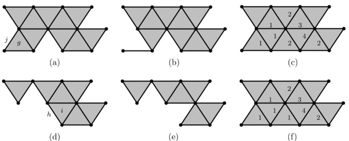
We ilustrate in fig. 8(a) a complex X where g is a border face of X and j is a free face of X. Fig. 8(b) depicts the set X \ {g, j} an elementary collapse of X.
Let us consider weights on the 1-faces of a complex. Let X * K, we denote by A the set of all 1-faces of X, and T the set of all 2-faces of X. Let us denote by F the set of all maps from A to R. Let F ∈ F, we will denote also by F the map from T to R such that for any g ∈ T , F (g) is the minimal weight of its 1-faces, i.e F (g) = min{F (u)|u ∈ A, u ∈ ˆg∗}.
j g (a) (b) 1 4 2 1 3 1 2 2 (c) h i (d) (e) 1 4 2 1 3 1 1 2 (f)
Figure 8: (a) A complex X and a free pair (j, g) for X. (b) An elementary collapse for X. (c) A weighted complex K with the map F on 1-faces (consider the 1-faces with no weight that have a weight greater than 4). (d) The section F2 of F . (h, i) is a free pair of F2. (e)
An elementary collapse for F2. (f) A border thinning of K.
We will define also for weighted complexes the lowering operation on 1-faces, as pre-sented for edge weighted graphs in def. 7.
Let u∈ A. The lowering of F at u is the map in F, denoted by [F \ u], such that: -[F \ u](u) = min{F (g), F (h)|g∩ h = u}; and
We denote Fk = {u ∈ A, g ∈ T |F (u) ≥ k, F (g) ≥ k} with k ∈ R, and we called it a
section of F .
Consider X be a complex in K and F ∈ F the weights on the 1-faces of X. Let Fk
be a section of F . We define also a 1-face u ∈ A a border 1-face for F if u is a free face for Fk with k = F (u). It can be seen an elementary collapse of a section Fk as a
low-ering operation on a border 1-face for F . Thus, we can observe an equivalence with the notions explained for border thinnings on edge-weighted graphs. Furthermore, this justify our choice of the vertex per-face graph as a representation for the mesh to proceed in a proper segmentation.
We illustrate with an example these previous notions. Consider the complex K depicted in fig. 8(c) with a map F . The figure only shows values on 1-faces which are lower than 4. 2-faces have the values corresponding to the minimal weight of its 1-faces. We illustrate in fig. 8(d) the section F2 of F , where h is a border 1-face for F , as it is a free face for
F2 and F (h) = 2. Fig. 8(e) depicts an elementary collapse of F2, and fig. 8(f) depicts
the lowering on the border 1-face h. In can be observed the equivalence with the border thinning explained in def. 8 applied on the vertex per-face graph of K.
4
Component tree
The component tree is a tree structure used to organize the connected components of a level function. It has been used for several image processing applications, although it was first introduced in statistics for classification and clustering. Different variations have been implemented as the Max-Tree introduced by Salembier et al. [19] used as a data structure for antiextensive connected operators, which is analysed and improved by Meijster and Wilkinson [12]. The algorithm we implemented is based on the one described by Najman and Couprie [14].
We will describe briefly the building process of the tree in order to give an idea of the properties of this structure, and later it will be introduced formally. The tree can be build as a Max-Tree (focusing on regional maxima) or a Min-Tree (focusing on regional minima), and for our purposes the Min-Tree approach has been used. Consider a discrete map as a topographical relief with the level of each point corresponding to its altitude. We will start flooding by water this surface starting at the lowest points. At beginning there will appear various lakes that will form the leafs of the tree. As water level increases the lakes will grow building the branches of the tree. By the time at some levels the lakes will merge into one connected piece becoming the forks of the tree. When the water reaches the highest level the process stops and the flooded area forms a unique component that is the root of the tree.
The tree can be used for filtering the original level function to obtain, for example as in our purposes, a new map with a reduced number of regional minima. Some attributes will be computed for each leaf and branches of the tree, and they will set an order of preference. As in the analogy explained before, the smaller valleys (considering their area for example)
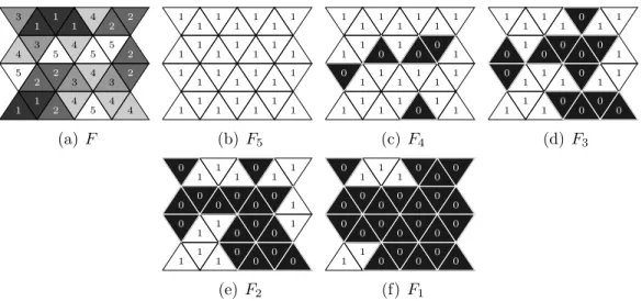
4 4 4 3 4 4 4 3 3 3 4 5 5 5 5 5 1 1 1 1 1 2 2 2 2 2 2 2 (a) F 1 1 1 1 1 1 1 1 1 1 1 1 1 1 1 1 1 1 1 1 1 1 1 1 1 1 1 1 (b) F5 1 1 1 1 1 1 1 1 1 1 1 1 1 1 1 1 1 1 1 1 1 1 1 0 0 0 0 0 (c) F4 1 1 1 1 1 1 1 1 1 1 1 1 1 1 1 1 0 0 0 0 0 0 0 0 0 0 0 0 (d) F3 1 1 1 1 1 1 1 1 1 1 1 1 0 0 0 0 0 0 0 0 0 0 0 0 0 0 0 0 (e) F2 1 1 1 1 1 0 0 0 0 0 0 0 0 0 0 0 0 0 0 0 0 0 0 0 0 0 0 0 (f) F1
Figure 9: A weighted face set F and its cross-sections at levels 5, 4, 3, 2, 1 (in white).
of the topographical relief will be removed. Hence, removing the corresponding branches of the tree.
We implemented a quasi-linear time algorithm for computing the component tree of functions defined on edge-weighted graphs that is based on the Tarjan’s union-find proce-dure [20]. We will define the component tree on the framework of graphs, and it will be illustrated with the case of a vertex-per-face graph on a complex as described in section 2.4. We will explain the union-find method and after introduce the algorithm to build the tree. Later we will describe the methods used for filtering the mesh curvatures values using the component tree in order to obtain the desired watershed segmentation.
4.1
Connected components notions
We introduce some notions and notations for connected components in weighted graphs in order to define properly the component tree in the following section.
We denote by F the set of all maps from E to R. For a map F ∈ F let us consider (V, E, F ) an edge-weighted graph. We also denote by F the map from V to R such that for any x ∈ V , F (x) is the minimal altitude of an edge which contains x. We define Fk = {u∈ E|F (u) ≤ k} with k ∈ R; Fk is called a (cross-)section of F . It can be noticed
that for any u ∈ Fk and x, y the vertices at u, also F (x) ≤ k,F (y) ≤ k. A connected
component of a section Fk is called a (level k) component of F . A level k component of
F that does not contain the level (k− 1) is called a (regional) minimum of F . We define kmin = min{F (u)|u∈ E} and kmax = max{F (u)|u∈ E}, which represent respectively the
minimum and the maximum level in the map F .
We illustrate this notions on the framework of triangular face sets with fig. 9 where the different cross-sections can be observed. In this case we have weights on faces, and their connectivity is determined by the vertex per-face graph explained in section 2.4.
4.2
Component tree definition
The following definition for the component tree is extracted from [14].
Let F ∈ F. For any component c of F we set h(c) = min{k|c is a level k component of F }. Note that h(c) = max{F (x)|x∈ c}. We define C(F ) as the set composed of all pairs [k, c], where c is a component of F and k = h(c). We call altitude of [k,c] the number k. Remark that any two distinct elements of C(F ) correspond to distinct subgraphs.
Let F ∈ F, let [k1, c1],[k2, c2] be distinct elements of C(F ). We say that [k1, c1] is the
parent of [k2, c2] if c2 ⊂ c1 and if there is no other [k3, c3] in C(F ) such that c2 ⊂ c3 ⊂ c1.
In this case we also say that [k2, c2] is a child of [k1, c1]. With this relation “parent”, C(F )
forms a directed tree that we call the component tree of F, and that we also denote by C(F ). Any element of C(F ) is called a node. An element of C(F ) which has no child is called a leaf, the node which has no parent is called the root.
We define the (vertex) component mapping CM as the map from V to C(F ) which associates to each vertex p∈ V the node CM(p), such that the altitude of CM(p) is F (p) and p ∈ CM(p). We also define the edge component mapping CME as the map from E to C(F ) which associates to each edge u∈ E the node CME(u), such that the altitude of CME(u) is F (u) and u∈ CME(u).
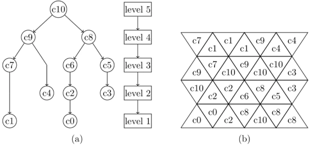
Fig. 10(a) shows the component tree of the vertex per-face graph of F the face weighted set of fig. 9 and fig. 10(b) shows the associated component mapping depicted on the faces of the set F . c10 c9 c7 c1 c4 c8 c6 c2 c0 c5 c3 level 5 level 4 level 3 level 2 level 1 (a) c8 c8 c9 c7 c9 c8 c8 c6 c5 c7 c9 c10 c10 c10 c10c10 c0 c1 c0 c1 c1 c2 c3 c4 c2 c2 c4 c3 (b)
Figure 10: The component tree (a) of the vertex per-face graph of the face weighted set of fig.9 and its associated component mapping (b).
4.3
Component tree and minimum spanning tree
As our work is settled on edge-weighted graphs, some considerations will be introduced in order to understand the algorithm for the construction of the component tree implemented, and its differences with the previous algorithms [14] [19].
We present the notion of line graph that will allow us to apply the notions for vertex-weighted graph on edge-vertex-weighted graphs.
Definition 9. The line graph of G = (V, E) is the graph (E, Γ), such that {u, v} belongs
to Γ whenever u∈ E, v ∈ E, and u and v are adjacent, i.e, |u ∩ v| = 1.
We can associate to each graph G whose edges are weighted by a cost function F , a line graph G′
. The vertices of G′
are weighted by F and thus any transformation can be performed either in G or in G′
.
We could apply the algorithm introduced by Najman [14], which focus on vertex-weighted graphs, on an edge-vertex-weighted graph G, by using the line graph of G, G′
. Then, once the component tree would be built, we would obtain the component mapping of the vertices E of G′
. Thus we would have the component mapping on the edges E of G. Then, by removing nodes of the tree, we would reduce the number of minima on the edge-weighted graph G.
The purpose of the filtering of a map F on edges of a graph G is to reduce the over-segmentation produced by the watershed operator. Considering this purpose our compo-nent tree will be computed only on the minimum spanning tree edges of the graph. On the following of this section we will explain this consideration.
As introduced in section 3.3 the watershed cut of F is induced by the minimum spanning forest relative of the minima of the map F . Furthermore, in section 3.3.1 we derived that the minimum spanning tree of a graph X is a MSF relative to the subgraph ({x},∅), x being any vertex of X.
Following the construction presented in section 3.3.1 we can state also the following. Let Y be the MSF relative to M(F ) for F in G. For any edge u ∈ Y \ M(F ) it can be observed that u belongs to a minimum spanning tree for F in G.
We will give some notations concerning minimum spanning trees (MST) in order to introduce later a theorem that will help us understand the approach adopted to construct the component tree.
Let us define a partition of the vertices of a graph G as a division into two disjoint non-empty subsets of vertices (P, Q). The distance ρ(P, Q) across a partition is the smallest weight among all edges which have one vertex in P and other in Q. The cut-set C(P, Q) is the set of edges that span a partition (P, Q). A link is any edge in C(P, Q) whose weight is equal to the distance ρ(P, Q), while the set of all links in C(P, Q) is called the link-set λ(P, Q).
A main theorem concerning a MST is the following.
Theorem 4. Any MST contains at least one edge from each λ(P, Q).
Let Y be a MSF relative to M(F ) for F in G, and X be any component of Y . Let P be the set V (X) and Q the set V (Y ) \ V (X). The cut-set C(P, Q) thus, belongs to the basin cut of F . By the theorem stated above it may be seen that the MST of F will contain the edge with lowest weight of C(P, Q).
Thus, by this latter considerations the MST will contain all edges of the MSF relative to M(F ) excluding the edges of M(F ) that make a cycle. Also, considering S the basin cut of F , the MST will contain any edge u ∈ S such that u is the lowest edge outgoing from a component of S.
Consider we obtain the component tree of G taking into account only the edges of the MST. Then we filter the map F by removing a branch of the tree. Hence we give at the nodes of the branch the level value of the parent of the highest node of branch. Let us call X the subgraph corresponding to the removed component. After the filtering, the edges not considered in the component tree, i.e edges that not belong to a MST, will get a ∞ value. We call this filtered map F′.
Consider now S the watershed cut of F , and S′
the watershed cut of F′
. Consider Y a component of S (a catchment basin). As the component X forms a branch of the tree, X ⊆ Y . We give to each edge of X the weight of the edge u ∈ S, such that F (u) is the lowest cost from the ones outgoing from Y , and also the edges of Y \ X get ∞ value. For this two latter reasons, there is no descending path from u in Y for F′
to M(F′
). Thus, Y is not a catchment basin for F′.
Our algorithm for the component tree is then based on a classical algorithm for the minimum spanning tree presented by Kruskal [9]. It consists in sorting first the edges of the graph by increasing order of their weight, and then selecting them, making sure to select only edges that do not form a circuit with the previously selected. In our case, during this stage we will proceed on the building of the component tree.
4.4
The Union-Find method
The Union-Find algorithm proposed by Tarjan allows keeping track of disjoint sets, per-forming three useful operations to manage a collection Q of disjoint sets. Each set is represented by an arbitrary member called the canonical element. The algorithm uses rooted trees to represent sets in which the root is chosen as the canonical element. Two objects x and y are members of the same set if and only if x and y are nodes of the same tree, which is equivalent to saying that they share the same root of the tree they are stored in. The collection is managed by the following operations:
• MakeSet(x): add the set {x} to collection Q. This operation assumes that x is not a member of any other set in Q.
• Find(x): return the canonical element of the set in Q which contains x.
• Link(x,y): let X and Y be two non empty set in Q represented by x and y (x and y must be different). Both sets are removed from Q, their union Z = X∪ Y is added to Q and a canonical element for Z is selected and returned.
The implementation of the algorithm is the one presented at procedure MakeSet and functions Find and Link. To each element x is associated a parent Par(x) and a rank
Rnk(x). A technique used to reduce the run cost of the function Find called path
com-pression consists, after finding the root r of a tree which contains x, in setting the parent
of each element of the parent path from x to r to be r. Another technique used is the one called union by rank. The rank Rnk(x) is incremented by one if x becomes parent of y. The technique consists in always choosing the representing element with the greatest rank while performing the Link operation. If both elements have the same rank one of them is chosen arbitrarly.
Procedure MakeSet(element x ) Par(x):=x; Rnk(x) :=0;
1
Function element Find(element x )
if (Par(x)$= x) then Par(x) := Find(Par(x));
1
return Par(x);
2
Function element Link(element x, element y) if (Rnk(x) > Rnk(y)) then exchange(x,y);
1
if (Rnk(x) == Rnk(y)) then Rnk(y) := Rnk(y) + 1;
2
Par(x):=y;
3
return Par(x);
4
4.5
Component tree algorithm
In this section we explain the algorithm implemented to build the component tree C(F ) on an edge-weighted graph in the context of a vertex per-face graph on a mesh surface. The algorithm is based on the one presented by Najman and Couprie with some modifications to better perform on edge-weighted graphs as explained in sec. 4.3. We first will describe the algorithm from a high point of view and later some details will be explained.
4.5.1 High-level view
The process will simulate a flooding as described before. This flooding is realized by scan-ning the edges of the graph by increasing order of their level. Two disjoint set collections Qnode and Qtree will be used to manage the merging of nodes and branches of the tree. As
edges are scanned by level increasing order, the vertices first time visited will get the mini-mum weight value of their adjacent edges. The elements needed to manage the collections Qnode and Qtree are build during the process. The Qnode collection will group vertices and
edges belonging to the same connected component and having the same altitude. Simul-taneously the Qtree collection will group the canonical nodes of each Qnode node to form
partial trees. At the end of the execution a unique tree groups all the canonical nodes, each of the nodes represents a component of the graph, and the whole tree represents the component tree.
4.5.2 Detailed view
The algorithm for the component tree computation is presented below BuildComponentTree, also with the complementary functions used, InitNode and MergeNodes. To represent a node of C(F ) we use a structure called node that contains its level and the list of nodes which are sons of this node. In a preprocessing step edges are sorted by increasing order of level (line 1). Then the process starts (line 3) proceeding by taking each edge of the graph starting by the lowest one. We use a label nblabs an the array CM (used for the resulting component mapping) to proceed properly on the generation of new nodes of C(F ) during the processing step.
The function InitNode creates new elements of collections Qnode and Qtree using the
procedure MakeSet described in section 4.4. It also creates a new node structure.
The array highestNode will help us to know the node with highest level from a partial tree during the processing, and it is necessary due to the particularities of the union-find algorithm.
From the algorithm we also obtain the edge component mapping CME. We do not describe this array on the text presented in BuildComponentTree but we give the precise assignments below.
The BuildComponentTree procedure have three main possible cases, which depend on the previously visited vertices. To know if a vertex has already been visited we use the array CM set at an initial value for all vertices, in a preprocessing step. Considering u∈ E the edge chosen and (x, y)∈ u the vertices at this edge, the three possibilities are:
• both vertices are visited for the first time; in this case (lines 4-6), as we proceed on edges by increasing order of their level, and vertices have the minimal value of their adjacent edges, both vertices have the same level and it equals the edge level F (u). Thus, a new node of level F (u) is build (function InitNode) and the vertices x, y will belong to this node, so the component mapping of x and y is set to the new label nblabs. The edge component mapping CME is set to the same label nblabs for u. • one vertex has been visited and the other is visited for the first time; in this case
(lines 7-13) we use the array CM to know which node the vertex x belongs to (x is the vertex already visited). Using then the function Find on the collections Qnode
and Qtree we get its canonical node xnode (line 8).
If the edge level is the same as xnode level, it means that the other vertex y should
have this level also, and it belongs to the same node (line 9). CME(u) is set to xnode.
In the other case if F (u) is greater than the level of xnode, a new node it is created,
and xnode (the node that represents x) becomes its son (lines 11-12). The elements of
new node as the highest on level of the partial tree recently build (line 13). CME(u) is set to the new node label.
• both vertices have been visited before; in this case we first find the canonical nodes that represent x and y (lines 15-16). In case that they are not in the same partial tree (line 17) we proceed differently depending on their levels.
If their level it is the same, nodes are merged (function MergeNodes)(line 22). CME(u) is set to the canonical node resulting from the merging.
If the edge level is equal than one of the nodes but greater than the other, the bigger becomes parent (line 24). CME(u) is set to the parent node.
If the edge level is greater than both nodes a new node is created, that becomes parent of both (lines 27-29). CME(u) is set to the parent node.
The partial trees are linked for this three preceeding cases.
The root of the component tree is found as the highest node of the resulting tree of the collection Qtree (line 33), while the component mapping is the resulting array CM.
Function node InitNode(int label, double level) Allocate a new node n with an empty list of children;
1
n→ level := level;
2
MakeSettree(label );MakeSetnode(label ); 3
return n;
4
Function int MergeNodes(int node1, int node2 ) tmpNode := Linknode(node1,node2 );
1
if (tmpNode == node2) then
2
Add the list of childrens of nodes[node1] to the list of children of nodes[node2];
3
else
4
Add the list of childrens of nodes[node2] to the list of children of nodes[node1];
5
return tmpNode;
Algorithm 7: BuildComponentTree
Data: (V, E, F ) - edge-weighted graph with N vertices Result: nodes - array [0 . . . N − 1]
Result: Root - Root of the component tree
Result: CM - map from V to [0 . . . N − 1] (component mapping) Local: highestN ode - map from [0 . . . N − 1] to [0 . . . N − 1] Sort the edges in increasing order of level for F ;
1
nblabs:=0;
2
foreach u∈ E in increasing order of level for F do
3
// u= (x, y)|x, y are vertices
if (both vertices are visited for the first time) then
4
nodes[nblabs]:=InitNode(nblabs,F (u));CM(x):= nblabs; CM(y):=nblabs ;
5
highestNode[nblabs]:=nblabs; nblabs ++ ;
6
else if (one vertex has already been visited an the other not) then
7
// considering x the vertex already visited
xtree := Findtree(CM(x));xnode := Findnode(highestNode[xtree] ); 8
if (F (u) == nodes[xnode]→ level) then CM(y):=xnode; 9
else if (F (u) > nodes[xnode]→ level) then 10
nodes[nblabs]:=InitNode(nblabs,F (u)); CM(y):=nblabs;
11
nodes[nblabs]→addChild(nodes[xnode]); 12
highestNode[Linktree(xtree,Findtree(nblabs))]:=nblabs; nblabs ++ ; 13
else if (both vertices already been visited) then
14
xtree := Findtree(CM(x));xnode := Findnode(highestNode[xtree] ); 15
ytree := Findtree(CM(y));ynode := Findnode(highestNode[ytree] ); 16
if (xnode $= ynode) then 17
if (nodes[xnode]→ level < nodes[ynode]→ level) then 18
temp:= ynode; xnode := ynode; xnode := temp ; 19
temp:= ytree; xtree := ytree; xtree := temp ; 20
if (F (u) == nodes[xnode]→ level == nodes[ynode]→ level) then 21
highestNode[Linktree(xtree,ytree)]:=MergeNodes(xnode, ynode); 22
else if ((F (u) == nodes[xnode]→ level)&&(F (u) > nodes[ynode]→ level)) 23
then
nodes[xnode]→addChild(nodes[ynode]); 24
highestNode[Linktree(xtree,ytree)]:=xnode; 25
else if (F (u) > nodes[xnode]→ level) then 26
nodes[nblabs]:=InitNode(nblabs,F (u));
27
nodes[nblabs]→addChild(nodes[xnode]); 28
nodes[nblabs]→addChild(nodes[ynode]); 29
highestNode[xtree]:=nblabs;highestNode[ytree]:=nblabs; 30
highestNode[Linktree(Linktree(xtree,ytree),Findtree(nblabs))] := nblabs; 31
nblabs ++;
32
foreach x∈ V do CM(x):=Findnode(CM(0)); 33
Root:= highestNode[Findtree(Findnode(CM(0)))]; 34