Dispersive prediction of single-screw extruder with mixing head using Boundary Element Method

HAL Id: hal-02056355

https://hal-mines-albi.archives-ouvertes.fr/hal-02056355

HAL is a multi-disciplinary open access

archive for the deposit and dissemination of sci-entific research documents, whether they are pub-lished or not. The documents may come from teaching and research institutions in France or abroad, or from public or private research centers.

L’archive ouverte pluridisciplinaire HAL, est destinée au dépôt et à la diffusion de documents scientifiques de niveau recherche, publiés ou non, émanant des établissements d’enseignement et de recherche français ou étrangers, des laboratoires publics ou privés.

Dispersive prediction of single-screw extruder with

mixing head using Boundary Element Method

Ibrahim Busuladzic, Fabrice Schmidt, Pierre Lafleur

To cite this version:

Ibrahim Busuladzic, Fabrice Schmidt, Pierre Lafleur. Dispersive prediction of single-screw extruder with mixing head using Boundary Element Method. International Conference of Polymer Processing Society„ Jun 2002, Guimarès, Portugal. �hal-02056355�

Distributive Mixing in a Single Screw Extruder Using

Boundary Element Method

Ibrahim Busuladzic (a), (b), Fabrice M. Schmidt (a), Pierre G. Lafleur (b), (a)Ecole des Mines d’Albi Carmaux (FRANCE),

(b)Ecole Polytechnique de Montreal (CANADA)

Abstract

The relationship between the mixing performance in extrusion and the process conditions is of great importance but is never easy to establish. Although experimental prototyping of mixing equipment provides insight into the mixing process, it is too time consuming and cost prohibitive to fully optimize the geometry and the process itself. Alternatively, numerical methods can be used to provide more detailed information on the mixing flows to alleviate the problems with experimental modeling.

The Boundary Element Method is an alternative technique which offers the possibility of modeling complex systems since it requires only the discretisation of the model boundaries. In this paper, we examine the use of a Boundary Element Method (BEM) model to predict the dispersive mixing performance of Maddock-like mixing heads on single screw extruders. We use this method to calculate the flow number on the middle plan of the studied geometries and compare it between different conditions of extrusion.

The experiments were conducted with a classical Maddock mixing head (in-house design). Two materials were extruded: a polypropylene/ calcium carbonate blend and a polyvinyl chloride/ red pigment blend. The numerical simulations were compared to the observed mixing behavior.

1- Introduction

Mixing is a very important process when we need final products with uniform properties. The state of dispersion (relative size of agglomerates) of filler minerals can be directly correlated to the dynamic and mechanical properties of composites (1-2). Such as in every polymer process, the mixing is a vital operation in single screw extrusion. Two types of mixing exist: Dispersive mixing and Distributive mixing.

Dispersive mixing involves the rupture of clumps and agglomerates of solid particles such as calcium carbonate or pigments. This rupture will happen only when the forces applied to the agglomerate or droplet exceed the forces keeping it together. In single screw extrusion, we use some devices to improve the mixing performance, like mixing heads, because dispersive mixing depends on the strain rates applied by the mixing devices. To realize our experiments we used Maddock like mixing heads. Classical Maddock mixing heads are primarily dispersive mixers. The material traveling through it is forced over the narrow flight gap before exiting the extruder. The other type of mixing, distributive mixing, spreads the dispersed or secondary phase throughout the primary phase or the mixture.

Beside the experimental studies to characterize mixing numerical analysis can be conducted. Various numerical methods have been used to simulate viscous creeping flows. In this numerical study we use The Boundary Element Method (BEM). The main attractiveness of BEM is that, for many applications, it provides the ability to reduce the dimensionality of the problem by one since only the boundary unknowns calculated in order to get the whole solution. Given the solution on the boundary, the unknowns inside the domain can be obtained.

2.1- Experimental study

The experiments were carried out on a 45 mm extruder. Two types of screw configuration are used: standard single screw and single screw with a Maddock mixing head Figure 1.

Figure 1. Geometry of spiral Madock head

The first test was to incorporate 5% of calcium carbonate into polypropylene. Then an extruded blown film was produced. The extruded film is transparent and can be observed with a microscope, see Figure 2.

Figure 2 – Sample of PPCOCa₃film

The dispersion is evaluated on 20 µm thick film. For the same conditions of extrusion we observed 30 samples from different parts of the film. In order to characterize the dispersion we used the model developed by Bories (3) to calculate the dispersion index f.

v f s i i i f W A d n f    6 3



Where

n

d

A

dispersion index f represents the volume ratio of agglomerates larger then 15μm and all secondary phase. agglomerat eral f  min   0

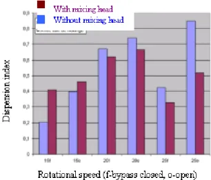
f can be greater then unity. Indeed, agglomerates are constituted of mineral, entrapped air and polymer, so their density is lower then the mineral’s density. The important extrusion parameters are: rotational speed, pressure and screw geometry. The average barrel temperature is 195°C. Rotational speeds are 15, 20 and 25 rpm. The results are shown in Figure 3. It can be noted that the effect of the mixing head is more important when we increase the rotational speed. Also, applying higher pressure leads to better dispersion states.

Figure3. Measured dispersion index for different conditions of extrusion

The second test was the extrusion of PVC band. The problem was to determine the dispersion of red pigment in PVC. The dispersion was determined counting the surface density of pigments. The average barrel temperature is 180°C. The rotational speeds used for those experiments are also 15, 20 and 25 rpm. The results are presented in Figure 4.

Figure 4. Experimental results quantifying dispersion of red pigment Best

dispersion

Worst dispersion

We note an important effect of the mixing head on the quality of the product ( i.e. dispersion of the red pigments).

2.2- Numerical study

The Boundary Element Method (BEM) offers the possibility of modeling complex systems since it requires only discretization of the model boundaries (4). BEM is also a convenient technique for modeling the rotating boundary problems such as the extrusion process because the domain only needs to be discretized once. The main disadvantage of BEM is the treatment of the non-linear problems. Where the method loses its principal’s advantages versus other numerical methods. Some techniques to deal with this problem exist such as Cell integration method or Dual reciprocity method (5).

In this study the polymer is assumed to be a Newtonian fluid and the flow process is considered isothermal. The momentum balance and continuity equation can be written as:

0    k jk x  (1) 0    k k x v ₍₂₎

Where jk is the total stress tensor and uk is the velocity vector. The stress tensor can be written as:

jk jk

jk p v

  2 (3)

Where p is the pressure, jkis the Kronecker symbol,  is Newtonian viscosity and vjkis the

rate of strain tensor. Finally we obtain the classical boundary integral equation.

0   

_

_

Where the multiplier ci depends on the location of point i and takes the value: ci 1when i is

inside the domain, ci 0.5on the boundary and ci 0 outside the domain.

*

jk

v and * jk

T are the velocity and traction components of fundamental solution respectively. The fundamental solutions correspond to the solutions in the j direction at a field point resulting from an infinite force applied in the k direction to the source point. In the case of viscous fluids for 3D problems we can write:









Where r is the distance between the source points and the points of calculation,

r

the projection of r in x, y and z direction. Knowing the external solutions we can obtain the solutions in every point of the domain (internal solutions) applying ci 1. In this study we

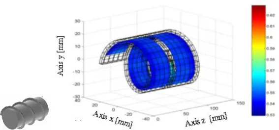
meshed the boundary using two dimensional quadrilateral isoparametric quadratic elements. We proceed to the BEM model assessment with the known analytical solution for a Couette flow. Rotational speed applied on the internal cylinder is 40rad/min. For this simulation we used 400

quadratic elements. CPU time is 1002 s. The total error comparing those two solutions for velocity are less then 0.25% and the same for velocity gradient are less then 3%, Figure 5.

Figure 5.Validation of the BEM simulation for Couette flow calculating the angular velocity error [%]

Numerical evaluation of mixing was done calculating the Flow number (6-7). The Flow number is a non-dimensional quantity that could be used to asses the flow type. The flow number is defined as:       _  (8)

Where  is the magnitude of the strain rate,  is the magnitude of the vorticity tensor. The maximum value for the flow number is 1 which represents an ideal elongational flow shown in Figure 6.

Figure 6. Elongational flow

Figure 7 shows the first simulation for the case of extrusion using single screw without mixing devices. The boundary conditions applied were simplified. The barrel is rotating and the screw is stationary (8). 802 quadratic elements were used for this simulation. We placed the internal points at the middle plane of channels where we calculate the flow numbers. CPU time is 140 min on IBM RS6000 station. In the case when we apply the rotating velocity of 20 rpm and the pressure difference of 300 kPa, one can see that the value of flow number is not more then 0.62. The average value of flow number is 0.54.

Figure 7 – Results for the flow number for the case of extrusion with single screw.

The geometry of a classical Maddock mixing head shown in Figure 1. can be divided into three identical section. Because the sections are identical the simulation is performed on two channels, as shown in Figure 8.

a). b).

Figure 8.-a) Geometry of mixing head, b) Part of the geometry to model and the boundary conditions.

We apply the following boundary conditions. The barrel is rotating and the mixing head is stationary. Because the flow rate is constant, we impose the known velocity of the polymer at the entrance and in the exit of the mixing head. The polymer is entering by the first channel, forced through the narrow gap and exiting by the second channel, Figure 8b. For this simulation we used 791 quadratic elements. 126 internal points were used and placed at the middle plane inside the geometry to calculate the flow number. For those simulations we worked with a constant flow rate and we used different rotational velocities to study the influence of this parameter on the flow number. CPU time is 125 min on IBM RS6000 station.

For the first simulation we worked with flow rate of 210g/min and we were applying the following rotational velocities a) – 15 rpm, b) – 40 rpm and c) – 25 rpm. The results are shown in Figure 9. We note that the flow number increases on the points entering the narrow gap. Inside this zone, the mixing head produces an elongational type of flow such as shown in Figure 6. The elongational deformation is more important then in others parts of mixing head. By increasing the rotational velocity, the flow number is increasing in the zone entering the narrow gap.

a) b)

c)

Figure 9 – Flow number distribution with flow rate of 210 g/min and different rotational velocities: a) – 30 rpm, b) - 40 rpm, c) - 50 rpm.

a) b)

c)

Figure 10 – Flow number distribution with the flow rate of 400g/min and with different rotational velocities: a) – 30 rpm, b) - 40 rpm, c) - 50 rpm

Figure 10 shows the flow number distribution where we used a constant flow rate of 400g/min. and different rotational velocities. In this case the factor of pressure difference is more important. With regard to the previous case, the average flow number is greater but is slightly weaker in the region of narrow entrance. Increasing rotational velocity yields higher flow numbers as in the previous case.

3- Conclusions

Experimental study on filler dispersions show that mixing heads are more efficient when we increase the rotational speed. Also increasing the pressure yields to better dispersions. For single screw without mixing head, increasing the rotational speed will result in a decrease of the quality of dispersion. A pressure decrease inside of extruder resulted in worse dispersion. PVC’s experiments show the necessities of using a mixing head. The rotational speed is a very important factor to get better dispersions, especially for the screw without mixing head.

Even though in this study the polymer is considered Newtonian, Boundary element method give us very quickly some useful information about the quality of mixing. For this study we have evaluated the dispersion calculating the flow number. Simulation for mixing heads shows that the presence of the elongational mode of the flow is important when the polymer is in the zone of the entrance in the narrow gap. Increasing the rotational speed will increase weakly the flow number. Also the effect of the flow rate caused by pressure difference is evident, producing higher flow number inside the overall geometry.

The numerical results highlight the dependence of the dispersion to pressure difference and to the rotational speed and are in god agreement with experimental results. These results are preliminary and a more elaborate dispersive model will be used to try to obtain quantitative comparison between the state of dispersion and the simulation.

4- References

1. Y.J. Suetsugu, Int. Polym. Proc., 5, 183 (1990).

2. Y.J. Lee and I. Manas-Zloczower, Polym. Eng. Sci., 35, 1037 (1995).

3. M. Boreis, “Influence des conditions opératoires d’extrusion sur la dispersion de carbonate de calcium dans une matrice de polypropilène”. (in French), M.A.Sc. Thesis, Ecole Polytechnique de Montreal, 1998.

4. C.A. Brebbia, J. Dominguez, “Boundary elements An introductory course”. Wit press/ Computational Mechanics Publications, 1992.

5. B.A. Davis, “Investigation of non-linear flows in polymer mixing using the boundary integral method”, Ph.D. Thesis 1995, University of Wisconsin-Madison.

6. P.J. Gramann, “Evaluating mixing of polymers in complex systems using the boundary integral method”, Ph.D. Thesis 1995, University of Wisconsin-Madison.

7. J. Cheng, I. Manas-Zloczower, Int. Polym. Proc., 5, 178, (1990).

8. C. Rauwendaal, T.A.Osswald, G. Tellez, P.J. Gramann, Int. Polym. Proc., XIII,(1998),4

With mixing head Without mixing head