Freeze/Thaw cycle monitoring using multi-scale SMAP products and hydrothermal modeling over the Canadian tundra: Final Research Report 2015-2019.

(1)

Freeze/Thaw cycle monitoring using multi-scale SMAP products

and hydrothermal modeling over the Canadian tundra

Final Reseach Report / 2015-2019

Presented to the Canadian Space Agency

Sheldrake Watershed, Nunavik

By

Monique BERNIER1_{, Ralf LUDWIG}2_{, Tahiana RATSIMBAZAFY}1_, Jimmy POULIN1_{, Lingxiao WANG}2_{, Philip MARZAHN}2_{and Chaima TOUATI}1

1_{Institut national de la recherche scientifique, Québec, Canada} 2_{Ludwig Maximilians Universitat, Munich, Germany}

INRS Research Report # R1854 May 31, 2019

(2)

ISBN : 978-2-89146-931-9 (version électronique)

Dépôt légal - Bibliothèque et Archives nationales du Québec, 2019 Dépôt légal - Bibliothèque et Archives Canada, 2019

(3)

3

Professeure Monique Bernier

Institut National de la Recherche Scientifique Téléphone : 418-654-2585

Télécopie : 418-654-2600

Courriel : Monique.Bernier@ete.inrs.ca

Final report / 2015-2019

Freeze/Thaw cycle monitoring using multi-scale SMAP products and hydrothermal modeling over the Canadian tundra

Abstract

The seasonal Freeze/Thaw (F/T) cycle is a major phenomenon in the climate system and plays an important role in ecosystem functioning by influencing the rate of photosynthesis and respiration of the vegetation, reducing evaporation, reducing the penetration of water into the soil and altering surface runoff. Boreal and arctic regions form a complex land cover mosaic where vegetation structure, condition and distribution are strongly regulated by environmental factors such as soil moisture and nutrient availability, permafrost, growing season length and disturbance. In these seasonally frozen environments, the growing season is determined primarily by the length of the non-frozen period. Variations in both the timing of spring thaw and the resulting growing season length have been found to have a major impact on terrestrial carbon exchange and atmospheric CO2 source/sink strength in boreal regions. The frozen soil mapping can be

improved by using the NASA SMAP instrument which has a Radiometer at L-band (1.20-1.41 GHz). In fact, SMAP is able to monitor the frozen soil because of its ability to sense the soil conditions through moderate land cover. The accuracy, resolution, and global coverage of the SMAP mission make possible a systematic updating of frozen ground maps and monitoring the seasonal F/T cycle. The main purpose of this project was to enhance the Canadian Plan for SMAP related F/T products by 1) Supporting a ground network in Northern Quebec as a Cal/Val site related to F/T products in Canada; by 2) Testing and validating the SMAP data to monitor F/T state over the Tundra and the Boreal Forest in Canada; and by 3) Developing a hydrothermal model to provide soil moisture and freezing/thawing information in high spatial and temporal resolution at a watershed level. The information is crucial to better understand small scale heterogeneities of F/T related landscape features and to close the scale gap between field monitoring data and SMAP F/T products.

(4)

(5)

5

List of Figures

Figure 1: Location of surface probes (green dots) operational in 2012-2013, Hudson Bay East Coast. ... 18 Figure 2: Surveyed sites near Umiujaq and along the Sheldrake River from 2014 to 2017 ... 19 Figure 3 Locations of temperature and soil moisture operational sensors in 2018 near the Nordic village of Umiujaq, in the Tasiapik valley and in the Sheldrake catchment, Nunavik, Quebec (Basemap Open StreatMap). ... 20 Figure 4: Annual Cycles of Soil Temperature and Soil Water Content retrieved from station “hum3” at 5-, 10-, and 25-cm depth (August 2017-August 2018). ... 22 Figure 5: Annual Cycles of Soil Temperature and Soil Water Content retrieved from station “hum4” at 5-, 10-, and 25-cm depth (August 2017-August 2018). ... 22 Figure 6: Annual Cycles of Soil Temperature and Soil Water Content retrieved from station “hum7” at 5, 10, and 25 cm depth (August 2017-August 2018). ... 23 Figure 7: Annual Cycles of Soil Temperature and Soil Water Content retrieved from station “Sheldrake4” at 5-cm and 10-cm depth (August 2017-August 2018). ... 23 Figure 8: PALSAR (L1.5) data processing ... 25 Figure 9 : PALSAR Freeze/Thaw algorithm processing ... 27 Figure 10 : Brightness temperature (TBh) correction for 27 August 2016 scene. (a) corrected with

the approach described in O’Neill and Chan (2012), Method A. (b) corrected with the

Normalization Method (Method B) . ... 32 Figure 11 : Brightness temperature correction per land cover type (Forest; Tundra; Wetland and Mixed vegetation) for August 27 2016, ascending orbit scene: (a) original TB data, (b) TB

corrected using Method B , (c) Original TB per land cover type and (d) final corrected TB using Method C. ... 33 Figure 12 : Brightness Temperature maps for August 27, 2016. (a) Original data, (b) Method A (O’Neill and Chan, 2012), (c) Method B, the proposed normalization approach, and (d) Method C (with land cover)... 35 Figure 13: WaSiM hydrological model framework ... 38 Figure 14: ERA-Interim reanalysis grid centers (red triangle) over the DEM of the watershed ... 39 Figure 15: Surface deposits map, generated by using previous surficial deposits maps (1:50,000) (Lévesque et al., 1988), (Jolivel and Allard, 2013), field data and high-resolution optical images. ... 39 Figure 16: Soil temperatures at 10 cm and 35 cm simulated by the WaSim Model at a lichen site from September 2015 to August 2016 and in-situ soil photographs. ... 40 Figure 17 : Processing steps: ① SMAP-L1C TB correction of water bodies per land cover type ② MOD10A1 aggregation ③ MODIS_IGB aggregation ... 46 Figure 18 : Brightness Temperature distribution for Forest and Tundra classes during

Freeze/Thaw cycle for July 01 (A), October 30 (B), February 29 (C), March 15(D), April 15 (E) and May 02 (F) 2016 ... 48

(8)

8

July 1st_{with MODIS snow cover fraction during 2016 Freeze/Thaw cycle... 49}

Figure 20 : 2016 Snow cover cycle deduced from installed in-situ camera at the Umiujaq

Northern Village (project Caiman, INRS). ... 50 Figure 21 : First runoff simulation results of WaSiM for the Sheldrake river watershed. ... 51 Figure 22 : Spatial WaSiM simulation results for thawing depth in the Sheldrake river watershed. Two states of the continuous modeling are shown (11 April 2015 vs. 08 October 2015). The dynamics of varying thawing depth are a function of climate forcing land cover and soil type. . 52

List of Tables

Table 1 : List of Canadian main products related to SMAP (Canadian Science Team, 2013) ... 13 Table 2 : Lichen and vegetation height measurements (cm) at each station. Three replicas were done by station except for the Sheldrake stations. ... 21 Table 3 : Freeze and thaw reference seasons (Backscatter coefficient, dB) ... 28 Table 4 : Validation results of SMAP F/T states classification at Umiujaq pixel with in situ soil temperature data (sensors: Hum-1 to Hum-5) compiled from October to December 2016: a) original ∆NPR and corrected ∆NPR with approaches A, B and C. ... 36 Table 5: ERA-Interim reanalysis dataset evaluation. ... 38 Table 6: Freezing and thawing periods length and dates from in-situ measurements at 6:00 PM and from SMAP ascending orbit images for the cycle 2016-2017. ... 42 Table 7 : Freezing and thawing periods length and dates from in-situ measurements at 6:00 AM and from SMAP descending orbit images for the year 2016. ... 42 Table 8 : Freeze/Thaw states extracted from the ratio HH/HV PALSAR images. ... 43

(9)

9

List of Abbreviations

AMSR-E Advanced Microwave Scanning Radiometer for EOS

SMAP Soil Moisture Active and Passive

SAR Synthetic-Aperture Radar

SMOS Soil Moisture and Ocean Salinity SSM/I Special Sensor Microwave Imager

MIRAS Microwave Imaging Radiometer using Aperture Synthesis PALSAR Phased Array type L-band Synthetic Aperture Radar NASA National Aeronautics and Space Administration

CSA Canadian Space Agency

EC Environment Canada

AAFC Agriculture and Agri-Food Canada

F/T Freeze/Thaw

RMS Root Mean Square

LPRM Land Parameter Retrieval Model

VWC Vegetation Water Content

JPL Jet Propulsion Laboratory CEN Center for Northern Studies

GIS Geographic Information System

GMAO Global Modeling Assimilation Office

NCEP National Centers for Environmental Prediction NCAR National Center for Atmospheric Research

NCDC National Climate Data Center

NNR (NCEP- NCAR) Reanalysis

STA Seasonal Threshold Approach

Teff Effective Temperature

TS Surface Temperature

TC Canopy Temperature

TBV Vertical Brightness Temperature

(10)

(11)

11

1. INTRODUCTION

1.1 PROBLEM DEFINITION

Seasonal terrestrial freeze/thaw (F/T) cycle is an important phenomenon in Earth’s climate system; it has a significant influence on ecosystem processes such as vegetation photosynthesis, soil respiration, evapotranspiration, soil water infiltration, surface runoff, frost heave, and annual ecosystem productivity (England, 1990, Way et al., 1997, Hayashi, 2013, McDonald and Kimball, 2005, McDonald et al., 2004, Nemani et al., 2003, Smith et al., 2004, Lagacé et al., 2002).

Boreal and arctic regions form a complex land cover mosaic where vegetation structure, condition and distribution are strongly regulated by environmental factors such as soil moisture and nutrient availability, permafrost, growing season length and disturbance. In these seasonally frozen environments, the growing season is determined primarily by the length of the non-frozen period. Variations in both the timing of spring thaw and the resulting growing season length have been found to have a major impact on terrestrial carbon exchange and atmospheric CO2 source/sink strength in boreal regions,

(Frolking et al., 1996, Randerson et al., 1999, Kim et al., 2011, McDonald et al., 2004). The timing of spring thaw in particular, can influence boreal carbon uptake dramatically through temperature and moisture controls to net photosynthesis and respiration processes (Jarvis and Linder, 2000, Tanja et al., 2003). With evergreen forests accumulating approximately 1% of annual net primary productivity each day immediately following seasonal thawing, variability in the timing of spring thaw can trigger total inter-annual variability in carbon uptake on the order of 30% (Frolking et al., 1996, Kimball et al., 2004, McDonald et al., 2004). Temporal variations in the onset of frozen conditions in the fall are also significant but generally have less impact on annual productivity due to the increased importance of other controls on vegetation photosynthetic activity such as photo-period length (Kimball et al., 2004). An accurate characterization of the spatial and temporal soil freeze and thaw state, e.g. the timing of F/T transitions and the duration of the frozen season, contributes substantially to the understanding of ecosystem function in northern biomes (Way et al., 1997, McDonald et al., 2004, Lagacé et al., 2002).

As conditions such as cloud cover and available sunlight do not influence the ability of satellite microwave remote sensing techniques to observe land surface properties, microwaves allow the potential for continuous, consistent acquisition of spatially explicit data that is useful for daily monitoring of the land surface properties, including soil conditions (e.g. humidity), vegetation water content and snow water equivalent at any time, day or night (Lagacé et al., 2002). Soil freezing refers to the process of the freezing of water in porous soil media. The water in the soil creates heterogeneity in electrical charge at the molecular level, which causes the molecule polarity. The soil freezing decreases the rotational energy of the molecule which has a positive linear relationship to the dielectric constant. Consequently, the soil dielectric constant is reduced as well as the backscattering energy. Frozen soil behaves like dry soil at the microwave frequencies.

Microwave sensors on board satellite are well adapted tools to monitor the F/T cycle over the Boreal and Arctic regions of North America (McDonald et al., 2004, Kim et al.,

(12)

12

like SSMI (Kim et al., 2011) or AMSR-E (Jones et al., 2007, Kalantari et al., 2009) have given encouraging results. The launch of SMAP mission in January 2015 is an opportunity to improve F/T mapping. It was initially designed to make coincident measurements of surface emission (Radiometer) and backscatter (Synthetic Aperture Radar) at L-band (1.20-1.41 GHz). These frequencies have the ability to sense the soil conditions through moderate land cover. After the technical failure of the radar component of the satellite in July 2015, the radiometer alone is operational for earth surface brightness temperatures measurements.

1.2 SMAP MISSION

The SMAP instrument which was designed to include both a Radiometer and a Synthetic Aperture Radar operating at L-band (1.20-1.41 GHz), operates on a near-polar, sun-synchronous orbit approximately 680 km above the Earth surface, with a 6AM/6PM Equator crossing and a 8-day repeat ground-track. The swath width is on the order of 1000 km, which provides global coverage every 3 days at the Equator, and every 1-2 days at mid and high latitudes. The 6-m diameter deployable mesh antenna with 40° incidence angle ensures a 40-km footprint for the radiometer and 30-km real aperture footprint for the radar which is no longer functional (Canadian Science Team, 2013).

The resolution and global coverage of the SMAP mission makes possible a systematic updating of frozen ground maps and monitoring the seasonal F/T cycle. The mission requirement is 80% classification accuracy over an annual cycle. This is actually not that stringent since most areas north of the 45 parallel are frozen for long continuous periods. Basic approach is to use classification agreement: % agreement; % false hits; % omission.

The post-launch phase was scheduled to start right after In-Orbit Checkout (IOC), 3 months after launch (May 2015). Validation of L1 products including brightness temperatures and backscatters was achieved 6 months after launch and the validated L1 products was delivered to data centers at October 2015. In contrast, the Cal/Val segment for L2 to L4 products last 12 months and end with delivery of soil moisture, F/T state and carbon fluxes products at Launch + 15 months (May 2016). Cal/Val of F/T and carbon products involves both pre- and post-launch activities. The items to be evaluated and calibrated were (Canadian Science Team, 2013):

• L1C_TB: Low-resolution brightness temperatures with a 40-km spatial resolution and available on a 36-km Earth grid;

• L1C_S0_HiRes: High-resolution radar backscatters with a 1 to 3-km spatial resolution and available on a 1-km Earth grid;

• L3_F/T_A: Daily global composite of the F/T state based on active data, with spatial resolution of 1 to 3 km, available on a 3-km Earth grid;

Led by JPL researchers, the selected SMAP FT algorithm would have required reference backscatter values for frozen and thawed states at 3 km resolution. The plan was to use Aquarius derived references for L3_F/T_A and update dynamically post-launch using SMAP SAR measurements. With the loss of the SMAP radar, strategies to

(13)

13

mitigate the loss of radar-based F/T product have been considered. Recent efforts have advanced techniques that use L-band passive microwave brightness temperature measurements to infer frost depth and landscape freezing and thaw using ground-based radiometers at the local scale and large-scale investigations with ESA’s Soil Moisture Ocean Salinity (SMOS) satellite (Kalantari et al., 2014, Rautiainen et al., 2012, Rautiainen et al., 2014, Rautiainen et al., 2016, Roy et al., 2015). This creates latency challenges in producing the L3 FT product during the Cal/Val period but also the importance to evaluate and calibrate the radiometer product (L1C_TB) over Canada tundra and boreal forest. As planned, the post-launch Cal/Val segment is followed by an extended monitoring phase that will last for the remainder of the SMAP mission.

1.3 CANADIAN SMAP PRODUCTS

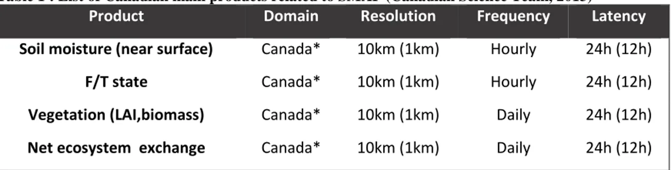
The science data products that are generated by the SMAP mission include; Level-1 Brightness Temperatures, Level-2 retrievals, Level 3- FT product and Level-4 modeling and data assimilation products. Although these official SMAP retrievals and data assimilation results are generated globally, some emphasis is expected for products over the US continental region which may not be optimal for the Canadian territory or for Canadian needs. It may therefore be advantageous for the Canadian project to generate another set of SMAP products specific to Canada. This products, listed in Table 1, are covering the Canadian territory and focus on targeted communities and scientific needs (e.g., agricultural risk assessment, numerical weather prediction, and hydrology). This imply application of different strategies for the generation of both retrievals and data assimilation products (soil moisture and F/T state), possibly involving the use of ancillary datasets more appropriate for Canada, as well as new (or at least different) retrieval algorithms and/or data assimilation techniques. The Canadian SMAP products includes retrievals for near-surface soil moisture and for the F/T state, as well as analyses (from data assimilation) of near-surface and root-zone soil moisture, F/T state, and carbon NEE. The Canadian Plan for SMAP (Canadian Science Team, 2013) includes a carbon component due to the crucial importance of northern regions in the global carbon cycle. For example, the considerable amount of carbon stored in permafrost may become available and be transferred to the atmosphere if thawing occurs. The F/T status of the soils also influences vegetation activity, to a degree even greater than that of soil moisture.

Table 1 : List of Canadian main products related to SMAP (Canadian Science Team, 2013)

Product Domain Resolution Frequency Latency

Soil moisture (near surface) Canada* 10km (1km) Hourly 24h (12h) F/T state Canada* 10km (1km) Hourly 24h (12h) Vegetation (LAI,biomass) Canada* 10km (1km) Daily 24h (12h) Net ecosystem exchange Canada* 10km (1km) Daily 24h (12h) *Global product will also be generated

(14)

14

The main purpose of this project (2015-2018) was to enhance the Canadian Plan for SMAP related to F/T products. The specific objectives were:

1. To support a ground network in Northern Quebec as the main Cal/Val site related

to F/T products in Canada. The main scientific objective of this core validation site is to provide field data for testing NASA SMAP products and to validate algorithms for monitoring F/T state over Canadian tundra and boreal forest sites.

2. To validate the effectiveness of L-band radar backscatters using PALSAR-2 to

monitor F/T state over the Tundra and the Boreal Forest in Canada.

3. To examine active/passive remote sensing synergies and assess sub-grid

heterogeneity in surface state and potential effects on soil frost dynamics over the Tundra and the Boreal Forest in Canada using radar data from PALSAR-2, RADARSAT-2 or Sentinel SAR and SMAP radiometer data.

4. To validate L1C_TB product (Low-resolution brightness temperatures with a

40-km spatial resolution and available on a 36-40-km Earth grid) to monitor F/T state at low resolution (40 km) over the Tundra and the Boreal Forest in Canada.

5. To develop (test) a hydrothermal model to provide soil moisture and

freezing/thawing information in high spatial and temporal resolution at a watershed level. The information is crucial to better understand small scale heterogeneities of F/T related to landscape features and to close the scale gap between field monitoring data and SMAP F/T products.

The Objective 2, 4 and 5 has been completed by March 31, 2018. For the extension year (2018-2019), the following activities were continuing:

- Objective 1 – To recover in situ data for testing NASA SMAP products and to

validate algorithms for monitoring F/T state over Canadian tundra and boreal forest sites.

- Objective 3 – To examine the active/passive remote sensing synergies,

integration of multi-sensors and multi-frequencies (TerraSAR-X, PALSAR-L, Sentinel-1 and SMAP radiometer data).

New objectives were also proposed for 2018-2019:

6. To publish in a Peer Review Journals the results of the validation of L-band radar

backscatters to map the F/T state and the assessment of the sub-grid heterogeneity (objectives 2 and 3) and the validation of the L1C_TB product (obj. 4) as well as the simulation results (obj. 5).

7. To address the problem caused by surface heterogeneity including the wet snow

cover during the thawing transitions in spring. We assume the SMAP radiometer data from the frozen soil underneath all land cover (snow cover, all type and size of vegetation covers) could be recovered by analysing backscattered echoes from PALSAR-2 and from other frequencies (C-band and X-band).

(15)

15

8. To use the hydrothermal model outputs by time step to close the scale gap between high resolution landscape features and satellite product, validate the results and assess the likely course of long-term permafrost dynamics in the region.

1.5 DOCUMENT ORGANIZATION

The next section presents the results achieved in relation with research Objectives 1 to 5. The third section described the results for the active/passive synergy and the objectives 6 to 8 which were specific for 2018-2019.

(16)

(17)

17

2. ACHIEVED RESULTS FOR OBJECTIVES 1 TO 5

2.1 OBJECTIVE 1 – CAL-VAL SITE IN DISCONTINUOUS PERMAFROST 2.1.1 Umiujaq-Sheldrake Cal-Val Site

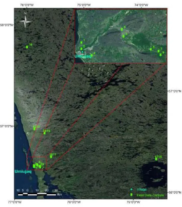
The validation site is located on the eastern shore of the Hudson Bay (QC) Canada in the Nunavik region (Fig. 1). It is a zone of discontinuous permafrost located at the tree line. This region has been the subject of more than 25 years of study by the Centre for Northern Studies (CEN). It is characterized by a complex landscape, including lakes, wetlands, marine, coastal, riparian, permafrost, streams. Back in 2010, data loggers were installed by INRS researchers near the village of Umiujaq (56.55° N, 76.55° O), to measure the water content and soil surface temperature over a few years. The soil texture was analyzed and land cover was also identified for each probe location (#1 to 9).

In summer 2012, soil temperature and TDR sensors were installed in three additional subarctic environments (Fig.1), dominated by thermokarst lakes and hollows; the Boniface River basin (#16) (57.45°N, 76.10°O), the Nastapoka valley (#12-14) (56.55°N, 76.22°O) and the Sheldrake River (#10-11) basin (56.36°N, 76.12°O), as well as in an open black spruce forest near Clearwater Lake (#17- 18) (56.51°N, 74.26°O). To access those watersheds, a helicopter was rented. A total of 17 specific sites were monitored from summer 2012 up to 2014. The sensors data were recovered in summer 2013, 2014 and 2015. Damaged sensors were replaced, except over the last two summers in the perspective of the end of the project in March 2018.

Near Umiujaq, two meteorological stations are operated by CEN, equipped with soil temperature probes for monitoring permafrost up to 20 m. Actually the recorded data are downloaded once a year during the onsite maintenance visit. In preparation of the launch of SMAP, a telecommunication system was installed to transmit the measurements in real time (daily) in a permanent meteorological station where soil temperature probes are already in place. The equipment shall be functional for a few years and the maintenance will be done by the CEN. Additional surveys were done in the summer of 2015, 2016 and 2017 and in winter 2016.

The purpose of those fieldworks were to get knowledge of the landscape in Sheldrake River catchment and Tursujuq National Park, to collect data about vegetation and soil properties, which has been used to parameterize the hydrological model (objective 5) and to simulate changes in the water balance in response to the dynamics in the hydro-thermal cycle of the subarctic region. Eight sites were surveyed along the Sheldrake River during summer 2014 (Fig. 2, green dots), all of them at helicopter reach. It is anticipated that each monitored site represents soil type and vegetation cover of one typical landscape. In these surveys, soil properties and land cover information were collected; thawing depths and soil moisture at several feature points were sampled through probing to provide additional data for the refinement and calibration of the hydro-thermal model (objective 5) and the high-resolution satellite imagery products (objective 2 and 3). In winter, snow cover properties were measured.

(18)

18

Figure 1: Location of surface probes (green dots) operational in 2012-2013, Hudson Bay East Coast.

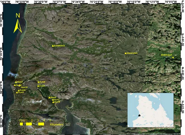
More sites being representative for typical local soil types, vegetation cover and snow cover properties were visited in summer 2015 to serve as ground control points for image analysis and point simulation results. Small black dots in Fig.2 show where photos were taken, either from the helicopter or on the ground. Those sites were re-visited during the summer 2016 and 2017 campaigns to monitor the annual thermal cycles.

(19)

19

Figure 2: Surveyed sites near Umiujaq and along the Sheldrake River from 2014 to 2017

2.1.2 Extension year in-situ activities

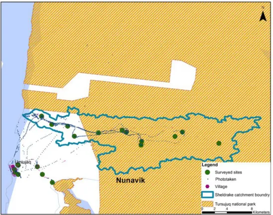
During the summer 2018, the team visited the Sheldrake River catchment. The main purpose of this fieldwork was to recover soil temperature data recorded at temporary stations since August 2017. Those data will be used to validate the 2016-2017 SMAP F/T maps and the WaSiM outputs. A helicopter was used to reach some surveyed sites. All the sensors in operation were kept in the soil for another year to increase the data sets for futher activities planned by the INRS-LMU team after March 2019. Fig. 3 shows the locations of the soil moisture and temperature sensors maintained by INRS in the Sheldrake catchment but also near the Nordic Village and in the Tasiapik Valley. Those later stations are accessible by the road.

(20)

20

Figure 3 Locations of temperature and soil moisture operational sensors in 2018 near the Nordic village of Umiujaq, in the Tasiapik valley and in the Sheldrake catchment, Nunavik, Quebec (Basemap Open StreatMap).

The aim of this fieldwork was first to verify the functionality of each of the mini-stations and to retrieve recorded temperature and soil moisture data from the previous year (Freeze/Thaw cycle 2017-2018). Vegetation height and mosses thickness over the soil were also measured during the field campaign at each station (Table 2). Three replicas were done by station within a distance of 10 m. These measurements are useful for analysing the satellite images, especially the radar (SAR) images for which the signal intensity is linked to the soil moisture, soil roughness and frozen state (PALSAR-2 L-band, Sentinel-1 C-Band, and TerraSAR X-Band). The objective 3 deals with the synergies between active (high resolution SAR data) and passive remote sensing (low resolution SMAP data) for assesing their complementarity for Freeze/Thaw monitoring, and evaluating heterogeneity in surface state.

Data collected in this survey will also be used to support the settings of a hydrothermal model to simulate water cycle and ground thermal conditions in the subarctic region with climate changing (objective 5).

(21)

21

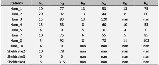
Table 2 : Lichen and vegetation height measurements (cm) at each station. Three replicas were done by station except for the Sheldrake stations.

Stations hl1 hv1 hl2 hv2 hl3 hv3

Hum_1 10 77 13 53 13 75

Hum_2 20 92 13 44 8 60

Hum_3 15 93 13 120 nan nan

Hum_4 15 58 8 60 10 53

Hum_5 4 0 5 0 4 0

Hum_7 10 75 6 55 5 85

Hum_8 5 92 8 78 11 103

Hum_10 4 0 nan nan nan nan

Sheldrake2 10 78 nan nan nan nan

hl and hv are lichen and vegetation height (cm) respectively.

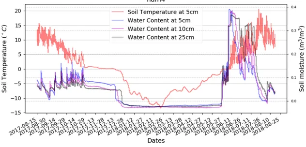
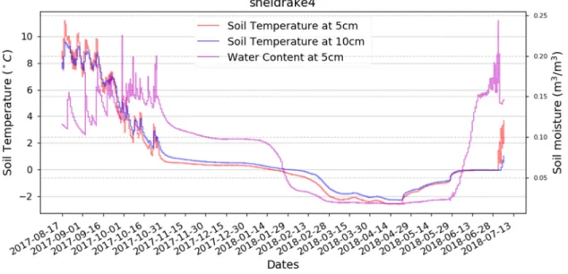
Figures 4, 5, 6 and 7, show the retrieved data from the stations “hum3”, “hum4”,

“hum7”, and “Sheldrake4” in August 2018. The Soil Temperature (TS) and Water Content (SWC) at different soil depths are presented in each of these figures. The retrieved data are time series of TS and SWC starting from August 2017 up to August 2018.

The SWC value at 5-cm depth is the double of the SWC at 10- and 25-cm depth at the station “hum3”. For the stations “hum4” and “hum7”, the SWC at 5-cm and 10-cm are approximatively the same during the freezing onset period. At 25-cm depth, the SWC is inferior to its values at 5- and 10-cm for “hum7”. The stations “hum3” and “hum7” are located near a stream. This would explain the higher value of SWC. At the “Sheldrake4” station, there is only one SWC sensor at 5-cm. The two TS values at 5-cm and 10-cm are close to each other. This station is beneath a grove of Black Spruce. The grove canopy acts as a shield from the cold air temperature in winter.

There are negative value of the SWC recorded during the freezing season in some soils. The sensor measuring the Water Content is not calibrated to measure absolute (accurate) values in clayey and/or organic soil. Nevertheless, the measured values were validated with soil sample collected from previous field works. The field work permitted to retrieve time series of Soil temperature and Soil Water content at different soil depth (5-, 10- and 25-cm). Each of the visited sensors were maintained and reinstalled to record data for the next Freeze/Thaw Cycle (2018-2019). The data would be recovered in summer 2019 and the sensors will recorded data at least up to August 2020.

Furthermore, all the soil temperature and soil water content data acquired since 2011 are now published and accessible openly on Nordicana-D (Bernier et al, 2019). Nordicana series D is a formatted, online data report series archived at the Centre d’études nordiques (CEN). It is freely and openly accessible. Nordicana-D has been conceived to ensure and maximize the exchange and accessibility of relevant data for the

(22)

22

situ data could be used by Environment Canada to validate the outputs quality of their new prevision system who assimilates surface data from SMOS, SMAP and GOES.

Figure 4: Annual Cycles of Soil Temperature and Soil Water Content retrieved from station “hum3” at 5-, 10-, and 25-cm depth (August 2017-August 2018).

Figure 5: Annual Cycles of Soil Temperature and Soil Water Content retrieved from station “hum4” at 5-, 10-, and 25-cm depth (August 2017-August 2018).

(23)

23

Figure 6: Annual Cycles of Soil Temperature and Soil Water Content retrieved from station “hum7” at 5, 10, and 25 cm depth (August 2017-August 2018).

Figure 7: Annual Cycles of Soil Temperature and Soil Water Content retrieved from station “Sheldrake4” at 5-cm and 10-cm depth (August 2017-August 2018).

(24)

24 2.2.1 PALSAR Data Processing

At microwave frequencies, liquid water and frozen have a large contrast. In fact, radar backscattering properties can be strongly sensitive to land F/T state. Active microwave data (Synthetic Aperture Radar (SAR) and Scattermeters) data has identified a sensitivity to near-surface soil moisture and land frozen or thawed states (Singhroy et al., 1992, Rignot et al., 1994a, Pulliainen et al., 1999, Bartsch et al., 2007, Kasischke et al., 2009). In fact, the water in the soil creates heterogeneity in electrical charge at the molecular level, which causes the molecule polarity. The soil freezing decreases the rotational energy of the molecule which has a positive linear relationship to the dielectric constant. Consequently, the soil dielectric constant is reduced as well as the backscattering energy (Wegmüller, 1990, Rignot et al., 1994b, Khaldoune et al., 2011, Park et al., 2011, Jagdhuber et al., 2014). Physical scattering models can explain successfully F/T transition but they are complex and require many input parameters and studies are limited to a small area. Radar data can be an effective tool to classify land state as freeze or thaw. Previous study prove that radar signal (co- and cross-polarization) can be useful to study thawed and frozen conditions (Kwok et al., 1994a, Kwok et al., 1994b).

Our validation of the F/T maps from the SMAP radiometer data (Obj. 4) shown the problem caused by surface heterogeneity within the satellite field-of-view including the snow cover during the freezing and thawing transitions in autumn and spring seasons and vegetation cover types. We would like to improve the F/T maps accuracy during the thawing transitions. We assume the SMAP radiometer data from the frozen soil underneath all land cover (snow cover, all type and size of vegetation covers) could be recovered by analysing backscattered echoes from PALSAR-2 (L-band, 1,27 GHz as SMAP). Though the combined analysis of F/T mapping result from sensors of different resolution (between 10m and 100m for PALSAR data and 36km for SMAP data), different working mode (active, PALSAR and passive, SMAP), it has potential to analyze and separate the different landscape and its component contributions to the signal. The PALSAR data were acquired to examine active/passive remote sensing synergies and assess sub-grid heterogeneity in surface state and potential effects on soil frost dynamics as well as mapping F/T states. PALSAR F/T mapping results will be used to validate SMAP F/T mapping and to understand what happen inside a particular 36km SMAP pixel, where high resolution PALSAR pixels don’t’ freeze or thaw at the same time. To validate passive and active F/T classification, Hobo- data loggers collected soil moisture and temperature from 5 cm depth were used.

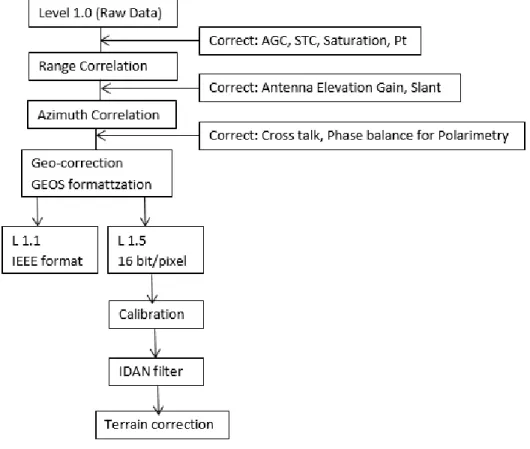
PALSAR data were acquired to examine active/passive remote sensing synergies and assess sub-grid heterogeneity in surface state and potential effects on soil frost dynamics. 100 PALSAR-1/2 images (L-band frequency) of the Japanese Advanced Land Observing Satellite (ALOS) over Turjusuk Park are investigated. Co-polarization (HH and VV) and cross-polarization channels (HV) signal sensitivity to vegetation and soil texture. PALSAR data (L1.5) are processed as shown in Fig. 8.

To convert digital number from PALSAR-2 products to backscattering coefficient (sigma naught, sigma zero) equations 1 and 2 are used. The radiometric and polarimetric calibration for the PALSAR-2 standard product (March, 2017) are:

(25)

25

For L1.5, L2.1 (1)

For L1.1 (2)

: Backscattering coefficient (Sigma naugh or Sigma zero) [db]

DN: Digital number (or raw pixel value)

CF1 and A: Calibration factors [db], respectively -83.0 and 32.0

In addition, polarimetric speckle filtering based on the Intensity-Driven Adaptive-Neighborhood (IDAN) filter was applied to obtain better performance in the change detection (Vasile et al., 2006, Fritz and Chandrasekar, 2008). Finally, we applied and validated for the Umiujaq-Sheldrake area the dynamic seasonal threshold from Kim et al. (2011).

(26)

26

The baseline SAR algorithm is established on a seasonal threshold approach (Rignot and Way, 1994, Way et al., 1997, Entekhabi et al., 2004, Khaldoune, 2006). Other SAR algorithms, based on moving window (Frolking et al., 1996, Kimball et al., 2001, Kimball et al., 2004, Rawlins et al., 2005, Kim et al., 2011) or temporal edge detection (McDonald et al., 2004) were also considered. The potential of ALOS-PALSAR data for F/T monitoring has been studied by McDonald (2011) in Alaska. This last algorithm examines the time series remote sensing signature relative to one or more reference signatures acquired during seasons when the signal is temporally stable, providing a seasonal reference state or states. This seasonal threshold approach works well for data with temporally sparse or variable repeat-visit observations such as SAR data and was to be used to produce an operational F/T product derived from L-band σ0_{every 3 days under}

the NASA SMAP mission (Entekhabi et al., 2010, Entekhabi et al., 2014).

Previous studies show that the seasonal changes of microwave backscatter can be subject to the vegetation types and their response to the temperature variation, rather than freezing of the ground soil (Park et al., 2011, Colliander et al., 2010). Colliander et al. (2012) evaluated the relative importance of the different landscape elements (vegetation stems and branches, soil of 5- and 10-cm depth) to the radar backscatter difference by tabulating the benchmarks of each backscatter-temperature combination (Colliander et al., 2012). Their evaluation shown the difficulty to clearly separate, from large footprint space borne observations, the different landscape contributions to the signal (Roy et al., 2015, Colliander et al., 2012).

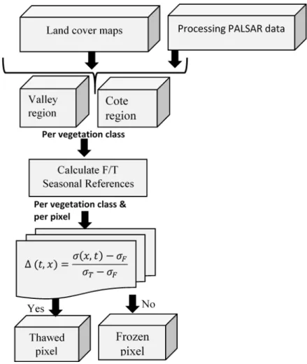
Freeze/Thaw cycle PALSAR-2 data algorithm (Fig. 4) is based on a seasonal threshold approach which has been adapted to match with Umiujaq land cover characteristics. Freeze seasonal references (January and February) and thaw seasonal references (July and August) are calculated per each vegetation type from Circa Land Cover of Canada (Latifovic et al., 2017). The algorithm examines the time series progression of PALSAR backscatter relative to backscatter values acquired during those seasonal references. A seasonal scale factor may be defined for a pixel x acquired at time t by equation 3:

(3)

Where:

is the measurement backscatter acquired at time t for a pixel x, is backscatter measurements corresponding to the frozen reference state (July, August),

is backscatter measurements corresponding to the thaw reference state for a pixel x (January, February).

(27)

27

Frozen if: (4)

Thawed if (5)

The algorithm is run on a cell by cell basis. The output is a dimensionless binary state variable: frozen or thawed condition for each PALSAR pixel.

Figure 9 : PALSAR Freeze/Thaw algorithm processing

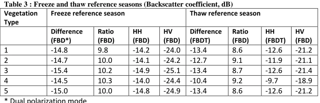
Table 3 shows freeze and thaw seasonal references for each vegetation type (1:

Shrubland, 2: Grassland, 3: Lichen/Moss, 4: Wetland, 5: Breen Land), for HH and HV polarizations. We also calculated the Difference and the Ratio values of the resultant HV and HV backscattering coefficient in decibel. The Ratio and the Difference are expressed as:

Ratio ₍₆₎

(28)

28

Table 3 : Freeze and thaw reference seasons (Backscatter coefficient, dB) Vegetation

Type Freeze reference season Thaw reference season Difference

(FBD*) Ratio (FBD) HH (FBD) HV (FBD) Difference (FBDT) Ratio (FBD) HH (FBDT) HV (FBD) 1 -14.8 9.8 -14.2 -24.0 -13.4 8.6 -12.6 -21.2 2 -14.7 10.0 -14.1 -24.2 -12.7 9.1 -11.9 -21.1 3 -15.4 10.2 -14.9 -25.1 -13.4 8.7 -12.6 -21.4 4 -14.5 10.3 -14.0 -24.4 -10.4 9.2 -9.7 -18.9 5 -15.0 10.0 -14.8 -24.9 -13.4 8.6 -12.6 -21.2 * Dual polarization mode

Results shows that backscatter coefficient (dB) decrease during the freezing season between 2 to 6 dB. A difference of 6 dB was measured for wetland pixels in HV polarization. Previous studies showed that C band backscatter coefficient (ERS and ENVISAT SAR data) decrease of about 3 dB between freezing and thawing states over tree species. A greater decrease was observed over tundra area (Rignot and Way, 1994, Wismann, 2000, Santoro et al., 2011). F/T maps are developed using PALSAR data.

Next steps are to validate the PALSAR results with in situ measurements, to compare PALSAR results with SMAP F/T classification for the Umiujaq pixel and write an article on the Active/Passive Synergy in L-band as proposed for Objective 3 for the extension year.

2.3 OBJECTIVE 3 - MULTIFREQUENCIES

2.3.1 Mapping permafrost landscape features with TerraSAR-X

In complement to Freeze-Thaw monitoring activities and modelling, the German collaborators mapped the permafrost landscape features with time-series TerraSAR-X images. Synthetic aperture radar (SAR)-based monitoring has become increasingly important for understanding the state and dynamics of permafrost landscapes at the regional scale. This study presents a permafrost landscape mapping method that uses multi-temporal TerraSAR-X backscatter intensity and interferometric coherence information. The proposed method can classify and map two important features in sub-arctic permafrost environments; 1) Permafrost-affected areas and 2) Thermokarst ponds. First, a Land Cover Map was generated through the combined use of object-based image analysis (OBIA) and classification and regression tree (CART) analysis. An overall accuracy of 98% is achieved for classifying rock and water bodies, and an accuracy of 79% is achieved for discriminating between different vegetation types with images in single-polarization acquired over one year. Second, the distributions of the permafrost-affected areas and thermokarst ponds are derived from the classified landscapes. Permafrost-affected areas are inferred from the relationship between vegetation cover and the existence of permafrost, and thermokarst ponds is a direct output of the land cover map. The two mapped features demonstrate good agreement with manually delineated references. This classification strategy can be transferred to other time-series SAR

(29)

29

datasets, like Sentinel-1 or PALSAR, and other heterogeneous environments. This research was published in the ISPRS Journal of Photogrammetry and Remote Sensing (Wang et al, 2018a).

2.3.2 Monitoring Thermokast pond dynamics with TerraSAR-X Data

Permafrost degradation can also be monitored through changes in the surface area and depth of thermokarst ponds. Radar remote sensing allows for discrimination of thermokarst ponds of different depths across large areas because different water depths produce different ice regimes in winter. In all, 28 TerraSAR-X images were used for this analysis, which covered a time range of 1 year. Fourteen images that were free of ground snow cover were regarded as summer acquisitions. The other 14 images with snow cover were regarded as winter acquisitions. The summer mean backscatter intensity image was used to distinguish the thermokarst ponds from other types of land cover. A supervised classification using the minimum distance classifier was applied. Because water bodies normally have lower backscatter intensities than land, high classification accuracy can be easily achieved (94% in our case study). The winter mean backscatter intensity image was used to classify the ice‐cover regimes of the thermokarst ponds. Because floating ice produces high backscatter intensity and grounded ice produces low backscatter intensity, the strong contrast allows these two ice‐cover regimes to be easily differentiated.

In this study, patterns in the spatial distribution of ice‐cover regimes of thermokarst ponds are first revealed. The ice‐cover regimes of thermokarst ponds are affected by soil texture, permafrost degradation stage and permafrost depth. In this study area, the first stage of the thermokarst process is the appearance of many small, shallow ponds with grounded‐ice in winter. Then, as all the ponds reach “maturity” (become fully developed), the average pond depth across the landscape increases, as does the proportion of ponds with floating ice. The segregation ice content and thawing depth of the permafrost, rather than the thermokarst pond age, control the water level of the thermokarst pond. The older ponds are greater in surface area than the younger ones but are not necessarily deeper (i.e., more ponds have the floating‐ice regime). The underlying soil texture (hydraulic conductivity) influences the speed of thermokarst pond drainage. Over the impermeable deposits, floating‐ice ponds generally have larger surface areas than the grounded‐ice ponds.

Permafrost degradation is difficult to assess directly from the coverage area of floating‐ice ponds and the percentage of all thermokarst ponds consisting of such floating‐ice ponds in a single year. Therefore, continuous monitoring of ice‐cover regimes and surface areas can help to elucidate the hydrological trajectory of the thermokarst process and. Using the freely available Sentinel‐1 SAR imagery and future RADARSAT Constellation data, the ice‐cover regimes and surface extents of thermokarst ponds can be recorded continuously. This studies is published in Permafrost and Periglacial Processus (Wang et al, 2018b).

(30)

30 2.4.1 Freeze-Thaw mapping algorithms

We acquired and analysed the SMAP 36-km spatial resolution brightness temperatures data (L1C_TB) over the study area from April 01, 2015. Previous approaches have used the TB (Brightness Temperature) or its spectral gradient to determine the soil frozen or non-frozen with satellite passive microwave images. The primary purpose of these techniques is to identify the transitions between frozen and non-frozen states. The commonest approach is temporal change detection. This approach supposes that observed large changes in microwave emissions are caused by the F/T transition and not by other factors, such as changes in the canopy structures, biomass, or precipitation.

Kim et al. (2011) have applied temporal change classification algorithm based on a seasonal threshold scheme to classify daily F/T states from time series TB measurements derived from SSMI images. They have used the 19 GHz and 37 GHz channels for deriving daily F/T classifications and selected the channel frequency, polarization, and channel combination having the highest global F/T classification accuracy relative to in situ air temperature measurements. According to their accuracy analysis, the best performance is achieved by a single frequency-based classification (37GHz V, pm, am).

The Seasonal Threshold Approach (STA) proposed by Kim et al. (2011) was then adapted to produce F/T maps to the SMOS TB time series. This dynamic threshold was estimated daily, pixel by pixel, using least-square linear regression between ΔTBp (x,t)

and the soil surface temperature as the independent variable, instead of the NCEP-NCAR reanalysis - air temperature at 2 m data in Kim et al. (2011) model. Kalantari et al. (2014) used a dynamic threshold level (ΔTB) derived for each year, on a grid cell-by-cell basis, using least-square linear regression relationship between surface temperature (independent variable) and ΔTB; then applied linear regression (mLR) to derive the negative slope between the TB and the water percentage of the ‘Lakes and Reservoirs’ (P) from the analyzed images. The estimated slope is then used for all pixels, but should be recalculated for each day. After testing and failing different scenarios, Kalantari et al. (2014) have used the weighting factor (a) for the class "Lakes and Rivers to eliminate the error caused by water emission from numerous lakes and rivers in each pixel. Then, after introducing the weighting factor (a) and processing separately the AM and PM data set, the Agreement Factor was improved to 81% for the SMOS AM data set.

In contrast from SMOS, the SMAP implementation allows 6:00 AM and 6:00 PM satellite overpasses to be used in combination to identify AM/PM difference in TB and classify those portions of the surface transitioning between frozen and thawed states. The SMAP radiometer data could then provide time series estimates of seasonal frost dynamics. For the low resolution data (L1C_TB), we used an INRS adaptation of the seasonal threshold approach proposed by Kim et al. (2011).

The NASA radiative transfer based approach proposed to correct the effect of water bodies on SMAP radiometer measurements (O’Neill and Chan (2012), Method A) is presented by equation 8.

(31)

31

(8)

TBgrid_{: raw brightness temperature in the data L1C_TB}

TBwater_{: Brightness temperature from water bodies}

TBland_{: Brightness temperature from land (Corrected TB).}

α: water proportion in each pixel of 36-km by 36-km (0%<α<100%)

By rearranging the equation to extract the , the factor (1-α) comes to the denominator side. As the water proportion α increase, the extracted TB from land tends to diverge when the water proportion starts to approach the value 50%. Then, we proposed two approaches to correct the SMAP L1C brightness temperature for the damping effect of water bodies inspired by Kalantari et al. (2014). The Temperature Brightness is known to decrease linearly within a region with high value of water proportion.

(9)

The first algorithm normalizes TB with the intercept of its linear regression versus the water fraction of each pixel within a scene (Normalization approach, Method B). Each TB values are presented as clouds of dots alongside the straight line presented by the equation 9. The new TB corrected is the normalized version of the old TB by respecting each of their orthogonal Euclidian distance from the regression straight line when they are normalized according to the intercept.

(10)

(11)

A second algorithm used Tb regression with water fraction by vegetation classes for each scene (Method C). An enhanced version of our method was conceived by applying the above correction for each of group of pixels sharing the same vegetation cover type as the vegetation density may disturb the thermal radiation emission coming from the first 5 centimeter of the soil surface. After being corrected from the “Lakes and Reservoirs” effect, the Normalized Polarization Ratio (NPR) is calculated for each pixel using the corrected Temperature Brightness in each polarization:

(12)

2.4.2 SMAP products used

SMAP L-band Brightness Temperatures (TB) in format Level-1C (L1C) were downloaded from the SMAP mission website. TB values are available in horizontal (TBH) and vertical (TBV) polarization and in fore- or aft-looking mode according to the antenna orientation along its track. The L1C products are the calibrated and geolocated version of TB in L1B. They are available on an Earth-fixed grid system with a spatial

(32)

32

(EASEv2) projection developed by the NSIDC (Brodzik et al., 2012). Two scenes of TB are recorded daily, which correspond to the satellite passes at 6:00 am (descending orbit) and 6:00 pm (ascending orbit) at local time respectively. The incidence angle of all acquisition is 40 degrees. Three years (2015, 2016, and 2017) of L1C TB were downloaded for the present study.

2.4.3 Freeze-Thaw mapping results

Figure 10 shows the results from the correction of the brightness temperature

according to NASA (Method A) and our approach (Method B). The TB values begin to diverge from the regression straight line when the water proportion inside the pixels grows to 30%. We suspect this divergence is a direct effect of (1-α) in the expression of

(equation 8). These artefact are not shown in the result of Method B. This is a particular advantage compared to the NASA approach.

Figure 10 : Brightness temperature (TBh) correction for 27 August 2016 scene. (a) corrected with the

approach described in O’Neill and Chan (2012), Method A. (b) corrected with the Normalization Method (Method B) .

The original TB values (red dots) varied between 143K and 259K with a std_diff of 4.44. After applying Method A, their values ranged from 172K to 317K with a std_diff value of 8.09. However, when Method B was applied, the new Tb ranged from 218K to 264K with a std_diff of 4.4. The corrected TB using Method A showed greater dispersion when compared to the non-corrected values for water fractions of 20% and greater. The visible dispersion of the TB values corrected with Method A is confirmed by the high value of the associated std_diff (8.09 for the corrected TB versus 4.4 for the original TB). Method B preserved the same dispersion parameter (std_diff = 4.4) before and after the

(33)

33

correction process. In fact, all pixels were corrected equally (with one regression line). This explains the conservation of the observed std_diff through the correction process in Method B.

Correcting brightness temperature from water surfaces effect depends on pixel land cover type. As illustrated by a previous study (O’Neill and Chan, 2012), correcting brightness temperature for bare soil pixels is easier than pixels with a dense vegetation.

Figure 11 shows the original SMAP brightness temperature data for August 27, 2016

(top left) covering Quebec and the TB values after normalization correction (top right). The original TB values for each of the four land cover classes (Forest, Tundra, Wetland, and Mixed Vegetation Cover) are shown individually in Figure 11c. After applying Method C, the TB values (TBC) ranged from 207K to 266K compared to 143K and 259K

for original data. Instead of being unchanged as in Method B, the standard deviation of the orthogonal distances of the corrected TB values was slightly higher (std_diff = 5.86 versus std_diff = 4.4). This was due to the number of regression lines used to produce TBC. Each intercept of pixels belonging to a given vegetation class was used to normalize

the original Tb values from those pixels. The TBC values of the “Forest” class had the

highest mean and those of the “Tundra” class had the lowest. Unlike soil covered with Forest, which acts as a temperature shield retaining heat in the soil underneath, soil covered with Tundra can easily lose its thermal energy. The differences between the corrected brightness temperature values of the soil within the four land cover classes explain the small increase seen in std_diff in the final TBC.

Figure 11 : Brightness temperature correction per land cover type (Forest; Tundra; Wetland and Mixed vegetation) for August 27 2016, ascending orbit scene: (a) original TB data, (b) TB corrected using Method B , (c) Original TB per land cover type and (d) final corrected TB using Method C.

(34)

34

Figure 12 shows brightness temperature maps for TB, TBA, TBB, and TBC. The

original data showed low TB values in the region north of 55 degrees (Fig. 12a). This region is characterized by a dense hydrological network (wetlands, lakes, rivers, and transient flooding). In addition to experiencing the damping effect of water surface on TB values, this region belongs to the “Tundra” land cover class, which is characterized by treeless and rocky land, where the heat energy in the soil can be transferred more easily to the atmosphere compared to soil under forests. The damping effect of water surface is more pronounced in the pixels located along the water/land boundaries in the north-west of the region (Kuujuarapik, Umiujaq, Inukjuak, Puvirnituq, Akulivik, Salluit, Quaqtaq and Kangipsualujjuaq). These pixels contain relatively high water fraction values compared to most inland pixels. The water fraction value reaches 40.5% for the Umiujaq pixel. This explains the necessity of masking ocean from land cover using high-resolution Landsat data. For brightness temperature map produced by the O’Neill and Chan (2012) approach (Fig. 12b), extremely high values of TB (represented by red pixels) can be seen in regions with a high water fraction. These values were caused by the greater dispersion of TBA noted earlier (Fig. 10a). This problem is not observed in the results from

proposed approaches B and C (Fig. 12c and Fig. 12d), where TB gradually decreases from south to north. The problem of low TB values observed along the north-west coastline boundaries is also solved.

Freeze/Thaw cycle monitoring for Umiujaq pixel using SMAP-L1C brightness temperature was validated using the field data from the installed probes. The probes recorded the physical temperature of the soil at 5cm depth hourly from August 23, 2015, to August 18, 2016, at five core sites. Probes sites are selected based on area representativeness (land cover, topography and soil texture). F/T classification produced from radiometer data collected during the two daily overpasses at 6 AM and 6 PM was validated using probe data recorded at the same time. For validation, stations with a sol temperature less than -1 degree Celsius or greater than 1 degrees Celsius at 6 PM or 6 AM were classified respectively as frozen or thawed. Between -1 and 1 degrees Celsius, the soil has been considered in F/T or T/F transition states (Wang et al. 2017). Table 4 summarizes the validation results of the estimated SMAP F/T states at the Umiujaq pixel against in situ F/T classification based on five soil temperature sensors installed in different locations (see table 1) in the ~36km SMAP pixel. The over level of agreement was calculated for ascending (A) and descending (D) overpasses using as input original brightness temperature (∆NPR) and corrected values with approaches A (∆NPRA), B

(35)

35

Figure 12 : Brightness Temperature maps for August 27, 2016. (a) Original data, (b) Method A (O’Neill and Chan, 2012), (c) Method B, the proposed normalization approach, and (d) Method C (with land cover)

(36)

36

Table 4 : Validation results of SMAP F/T states classification at Umiujaq pixel with in situ soil temperature data (sensors: Hum-1 to Hum-5) compiled from October to December 2016: a) original ∆NPR and corrected ∆NPR with approaches A, B and C.

Results illustrate that SMAP brightness temperature corrected with TB normalization per land cover type (approach C) shows better F/T agreement compared to approaches A (O’Neill and Chan approach) and B (Normalization approach) both for ascending (PM) and descending (AM) satellite overpasses. For the five sensors, the best agreement was obtained when land cover class information was incorporated in the brightness temperature correction process. Use of land cover type improved F/T agreement with the in situ data. F/T overall accuracy with approach C reaches 91% and 84% respectively for ascending and descending orbits. An improvement of up 24 % was measured on PM overall accuracy when approach C was used instead of approach A. In fact, as shown before method B conserves the same dispersion parameter value (std_diff) before and after TB correction from water effects. As expected, F/T agreement was higher than with the original TB, increasing from 70% to 74% for the ascending orbit and from 68% to 72% for the descending orbit. For some sensors, the results obtained from original ∆NPR showed better agreement than those with ∆NPR corrected using Method A (Hum-1 (PM), Hum-2 (PM) and Hum-5 (AM and PM). For Hum-5, the agreement decreased from 86% for original ∆NPR to 74% for corrected ∆NPRA acquired in ascending orbit and from

85% to 71% for descending orbit. This was a consequence of the divergence of the corrected TB values shown in Figure 10a since the water fraction used in the correction of Tb (see Equation 9) is relatively high (40%) in the pixel covering Umiujaq. Water surfaces such as lakes freeze progressively from their boundary to the middle, a process that the water fraction value used in Equation (9) does not take into account. By contrast, Methods B and C implicitly consider the overall variation of the TB values through the linear regression model used to normalize the TB values within a scene.

Sensors Original ∆NPR Corrected ∆NPR

Approach (A) Approach (B) Approach (C) Overpasses A(PM) D(AM) A(PM) D(AM) A(PM) D(AM) A(PM) D(AM)

Hum-2 71% 65% 67% 72% 74% 68% 90% 79% Hum-4 70% 67% 66% 74% 72% 73% 90% 85% Hum-5 64% 60% 67% 73% 71% 69% 90% 80% Hum-6 59% 65% 59% 78% 65% 72% 91% 86% Hum-7 86% 85% 74% 71% 86% 77% 96% 88% Overall accuracy 70% 68% 67% 74% 74% 72% 91% 84%

(37)

37

The same behaviour with respect to PM and AM F/T classification agreement results with in situ data has also been observed in previous studies, agreement with the PM F/T classification being generally stronger. For approach C, an overall accuracy of 91% was estimated for PM F/T classification instead of 84 % for AM F/T classification. Kim, Kimball et al. (2017) estimated mean annual agreements of 90.3% and 84.3% for PM and AM overpasses, respectively, for 36 years (1979–2014) over the global domain based on comparison of daily F/T classifications at 25 km using Special Sensor Microwave Imager (SSM/I), Scanning Multichannel Microwave Radiometer (SMMR), and SSM/I Sounder (SSMIS) data with F/T observations from global WMO weather stations. A previous version of the same study (Kim et al. 2011) showed mean annual agreements of 89.7% (PM) and 82.4% (AM). The sensitivity of these F/T state dynamics to the time of day of the overpass is related to the carbon cycle and the surface energy balance (McDonald and Kimball, 2005; Kim et al., 2011). The lower agreement for F/T classifications associated with AM overpasses may be explained by the drop in surface air temperature (SAT) during night-time (i.e. net radiation) and more significant variation in annual TB recorded in the AM overpass compared to the warmer TB in the PM overpass (Owe and Van De Griend 2001).

2.5 OBJECTIVE 5 - MODELING AT THE WATERSHED SCALE

The modeling studies was conducted in the wider Umiujaq area, including the Sheldrake River watershed, which is a 220 km² river catchment in the discontinuous permafrost zone on the east coast of Hudson Bay. The test site is selected due to its ideal suitability for the research question, a long research history(Allard and Seguin, 1987) (Allard et al, 1987; Lévesque et al, 1988, Jolivel and Allard, 2013), lots of cumulated ground observation data in this area, and its proximity to the CEN research station in Umiujaq. Hydrological model WaSiM with heat transfer module is adopted to describe hydro-thermal processes in watershed at 30m*30m resolution. It is a physically based, spatially distributed model, using the Richards-equation to describe water fluxes in the unsaturated soil zone, integrated with a multi-layered 2D-groundwater calculation. Snow accumulation and melt will be simulated using temperature-index-approach or an energy balance scheme, taking an accounting for wind-driven lateral snow redistribution (Warscher et al., 2013). Fig. 13 shows work flow of hydro-thermal model.

Input data includes meterological data and spatial grids. Facing the data scarcity, continous reanalysis dataset was adopted as meteorological inputs. The performance of two reanalysis datasets (ERA-Interim and NARR) were evaluated. They were compared with the measurements from Envionment Canada and CEN monitoring network in the eastern shore of Hudson Bay. ERA-Interim dataset got superior perfermance (Table 5). Its grid centers are shown in Fig. 14. For model calibration, the parameters were adjusted to fit measurements at the Sheldrake gauging station (Jolivel and Allard, 2013) using the NSE efficiency criterion.

(38)

38

Figure 13: WaSiM hydrological model framework

To calibrate the parameters in the heat transfer module, temperature profiles from boreholes (near Umiujaq airport) or deep temperature loggers (Nordicana D dataset, CEN), were used as well as a surface deposits map (Fig. 15) (Jolivel and Allard, 2013) and the active layer thicknesses measured in field campaigns.

Table 5: ERA-Interim reanalysis dataset evaluation.

Term

Number of Meteorological

stations for evaluation

Daily Weekly Monthly

NSE NSE NSE

Temperature 15 0.96 - 0.99 0.97 - 1.00 0.98 - 1.00 Precipitation 3 0.39 - 0.46 0.57 - 0.65 0.64 - 0.78 Relative humidity 6 -0.54 - 0.68 -0.06 - 0.66 -0.30 - 0.63 Radiation 3 0.79 - 0.85 0.87 - 0.93 0.86 - 0.94 Wind speed 10 -0.04 - 0.79 -0.04 - 0.75 -0.05 - 0.87

(39)

39

Figure 14: ERA-Interim reanalysis grid centers (red triangle) over the DEM of the watershed

Figure 15: Surface deposits map, generated by using previous surficial deposits maps (1:50,000) (Lévesque et al., 1988), (Jolivel and Allard, 2013), field data and high-resolution optical images.

This physically based and spatially explicit hydrological and hydrothermal modeling, built upon high-resolution remote sensing retrievals and field campaigns, can provide soil moisture, soil temperature and thawing depth information at daily step and 30 m resolution. Fig. 16 shows an exemple of outputs. The simulation of the soil temperatures at 10 cm and 50 cm from Septembre 2015 to August 2016.

The simulated soil temperature, moisture and thawing depths will serve as reference dataset when comparing the SMAP F/T products and F/T states retrieved from high-resolution ALOS2/PALSAR data for analyzing their consistency/inconsistency (Objective 8).

(40)

40

Figure 16: Soil temperatures at 10 cm and 35 cm simulated by the WaSim Model at a lichen site from September 2015 to August 2016 and in-situ soil photographs.

(41)

41

3. EXTENSION SPECIFIC ACTIVITIES

3.1 OBJECTIVE 3: ACTIVE/PASSIVE SYNERGIE and MULTIFREQUENCIES DATA INTEGRATION

3.1.1 Potential of C-band Sentinel-1 data to monitor F/T states

In 2017, the German collaborators started to study the potential of C-band Sentinel-1 data to monitor F/T states and this activity was pursued with INRS colleagues in 2018-2019. Recent research done by (Duguay et al., 2015) in this shrub tundra environment shows that soil moisture and temperature play a significant role in the backscattering coefficients, even in the presence of shrub vegetation and snow, which reveals that ground scattering remains a major component of the total backscattered power at C-band. The interferometric wide swath (IW) and extra-wide swath (EW) modes of Sentinel-1 offer 250km and 400km swath widths respectively. The pixel spacing is 10 × 10 m for the IW model Full resolution GRD product, 25 × 25 m for the EW mode Full resolution GRD product (Torres et al., 2012). The temporal repeat cycle is 6 days, when using Sentinel-1A and Sentinel-1B satellites.

A least square fitting of piecewise step function is used to determine F/T transition dates. The concept is to determine the transition date by minimizing the sum of squared residuals between time-series backscatter and the piecewise step function (Park et al., 2011). This method is adopted because of the weekly temporal repeat cycle of Sentinel-1. Some factors like wet snow and ice crusts formed by the melting and refrozen of surface snow layers introduce false F/T state result for a given scene. Previous studies demonstrated the approach could provide accurate FT transition timing from the noisy time series backscatter (Park et al., 2011). If the time-series backscatter has a gradual change during the finite time window, the break point in piecewise fitting infers a mean date of the variation period (Park et al., 2011). The team improved the method by using the backscatter evolution pattern instead of the noisy backscatter time series to determine the function parameters. Moreover, we are taking account of open water bodies which have a particular behavior and areas having an ambiguous F/T transition signal, like rock outcrops and the bare sandy area where soil moisture level and change is very low.

This study has not been published yet but the INRS-LMU team wishes to submit a manuscript over the next months who will compare the F/T transition dates of C-band Sentinel-1 data with the L-band sensors results (Objective 2 – PALSAR, Objective 4 - SMAP) to study the influence of frequency on the signal penetration depth and the scale effect brought by the landscape horizontal heterogeneity (water bodies, rock outcrops, wetland, sandy area,…) and vertical heterogeneity (soil/snow/vegetation) within the large satellite footprint observations (Derksen et al., 2017). We are exploring the synergy between C-band and L-band in shrubs and tundra environments. Time series backscatter data from each sensor is validated with soil temperature in situ measurements (Section 2.1).