Pépite | Identification des principales sources et origines géographiques de PM10 dans le nord de la France

Texte intégral

(1)Thèse de Diogo Miguel BARROS de OLIVEIRA, Lille 1, 2017. Nº d’ordre : 42289. THESE présentée en vue d’obtenir le grade de. DOCTEUR en : Spécialité : Optique et Lasers, Physico-Chimie, Atmosphère. par. Diogo Miguel BARROS de OLIVEIRA Titre de la thèse :. « Identification of the main sources and geographical origins of PM10 in the northern part of France » Soutenue le 27 Janvier 2017 Jury: Rapporteur Rapporteur Examinateur Encadrante Encadrant Encadrant Directrice de Thèse. Willy MAENHAUT Jean-Luc JAFFREZO Matthias BEEKMANN Esperanza PERDRIX Stéphane SAUVAGE Olivier FAVEZ Véronique RIFFAULT. Professeur, Ghent University Directeur de Recherche CNRS LGGE Directeur de Recherche CNRS LISA Maître-Assistante, Mines Douai Maître-Assistant, Mines Douai Ingénieur d'Etude et Recherche, INERIS Professeure, Mines Douai. Laboratoire d’accueil : Département Sciences de l’Atmosphère et Génie de l’Environnement, IMT Lille Douai. Ecole Doctorale SMRE 104 (Lille I, Artois, ULCO, UVHC, Centrale Lille, Mines Douai). © 2017 Tous droits réservés.. lilliad.univ-lille.fr.

(2) Thèse de Diogo Miguel BARROS de OLIVEIRA, Lille 1, 2017. © 2017 Tous droits réservés.. lilliad.univ-lille.fr.

(3) Thèse de Diogo Miguel BARROS de OLIVEIRA, Lille 1, 2017. Para a minha família Em especial para o meu avô, Victor Oliveira. © 2017 Tous droits réservés.. lilliad.univ-lille.fr.


(5) Thèse de Diogo Miguel BARROS de OLIVEIRA, Lille 1, 2017. ACKNOWLEDGEMENTS I would like to start by thanking Ecole des Mines de Douai and INERIS for co-funding this thesis and trusting in me to embrace this project. A special thanks to Mines Douai in the form of its Director, Patrice Coddeville and its Research Director, Nadine Locoge for having me during these 3 years. To the jury committee, Matthias Beekmann, Willy Maenhaut and Jean-Luc Jaffrezo a thank you for accepting to review my work and for your comments and advices on it. A special thank you to all my supervisors, Véronique Riffault, Olivier Favez, Esperanza Perdrix and Stéphane Sauvage, for being much more than that. To Véronique, for all the knowledge shared, the help and the time provided, but also for being someone to whom I could go to and talk about everything. To Olivier, for his help on my introduction to the subject, advices and guidance during this work and his friendliness and kindness shown since day 1. To Stéphane, for his valuable help on PMF and all its mysteries. Finally, a special thanks to Esperanza, not only for the incredible work support that always showed, for the always interesting scientific discussions we had, but also for being there since the beginning, helping me adjusting to this new reality. I also have to thank Aude Pascaud, for her help, kindness and patience during these 3 years. To Laurent Alleman, for his knowledge and advices on ICP and EC/OC analysis, uncertainties and PMF. To Bruno, for his help with the EC/OC instrument and always the funny conversations had (even if I was just understanding half). A big thank you to all my colleagues in the Department SAGE, and special thanks to those that became so much more than that - Thérése, Malak, Alexandre, Waed, Habib, Berenice, Shouwen, Evi, Antoine, Laura, Roger – this last for his insights on the troubled political situation in Cataluña and “gains” motivation. To my friends, a group that stuck together since university and was a huge support during these 3 years – no need to name anyone, vocês sabem quem são. A special and the most important aknowlegment goes to my family, my parents Jorge e Inês, and my brothers Joka, Rico and Kuka, for the constant support and love. And to Sofaki, I’m leaving Douai and Lille complete. We did it.. © 2017 Tous droits réservés.. lilliad.univ-lille.fr.


(7) Thèse de Diogo Miguel BARROS de OLIVEIRA, Lille 1, 2017. TABLE OF CONTENTS Acknowledgements .................................................................................................................... 5 Table of figures ........................................................................................................................ 13 List of tables ............................................................................................................................. 17 General introduction ................................................................................................................. 21 CHAPTER 1 - Bibliography on Composition and sources of tropospheric aerosols .............. 27 1.1. Particulate matter ....................................................................................................... 27. 1.1.1. Sources of PM10 ................................................................................................. 28. 1.1.2. PM10 composition ............................................................................................... 30. 1.2. Impacts and Regulation ............................................................................................. 37. 1.2.1. Climate impact of PM ........................................................................................ 37. 1.2.2. Health impact of PM .......................................................................................... 39. 1.2.3. Regulations ......................................................................................................... 41. 1.3. Source apportionment ................................................................................................ 42. 1.3.1. Source apportionment studies worldwide .......................................................... 45. 1.3.2. Source apportionment in Northwestern Europe ................................................. 47. 1.4. Geographical location of sources .............................................................................. 54. 1.5. Objectives of the thesis and scientific strategy .......................................................... 56. 1.5.1. Objectives of the thesis ...................................................................................... 56. 1.5.2. Scientific strategy ............................................................................................... 57. CHAPTER 2 - PM10 chemical speciation: measurements and results ..................................... 61 2.1. The CARA program .................................................................................................. 61. 2.2. Sampling sites ............................................................................................................ 62. © 2017 Tous droits réservés.. 2.2.1. Lens (urban site) ................................................................................................. 63. 2.2.2. Nogent-sur-Oise (urban site) .............................................................................. 65. 2.2.3. Rouen (urban site) .............................................................................................. 66. 2.2.4. Revin (remote site) ............................................................................................. 67. lilliad.univ-lille.fr.

(8) Thèse de Diogo Miguel BARROS de OLIVEIRA, Lille 1, 2017. 2.2.5 2.3. Roubaix (traffic site) .......................................................................................... 68. PM10 characterization methodologies ........................................................................ 69. 2.3.1. Filter sampling.................................................................................................... 69. 2.3.2. PM10 automatic measurement ............................................................................ 70. 2.3.3. Offline chemical analyses .................................................................................. 70. 2.3.4. Limits of detection ............................................................................................. 71. 2.3.5. Measurement uncertainties ................................................................................. 73. 2.3.6. Ion balance ......................................................................................................... 79. 2.3.7. Mass closure ....................................................................................................... 83. 2.4. PM10 chemical composition at each site .................................................................... 88. 2.4.1. Carbonaceous aerosols ....................................................................................... 92. 2.4.2. Organic species .................................................................................................. 95. 2.4.3. Ions ................................................................................................................... 101. 2.5. Exceedance episodes ............................................................................................... 104. 2.6. Conclusions of Chapter 2 ........................................................................................ 109. CHAPTER 3 - “Combination of Positive Matrix Factorization and Concentration Field methodologies to investigate the sources and geographical origins of PM10 chemical species: a French urban site case study” (Publication 1) ........................................................................ 113 3.1. Summary of Publication 1 ....................................................................................... 113. 3.1.1. Chemical analysis – Methods and results ........................................................ 113. 3.1.2. Source apportionment ...................................................................................... 115. 3.1.3. Source location ................................................................................................. 116. Combination of Positive Matrix Factorization and Concentration Field methodologies to investigate the sources and geographical origins of PM10 chemical species: a French urban site case study ............................................................................................................................... 117 1. Introduction .................................................................................................................... 119. 2. Methodology .................................................................................................................. 120 2.1. © 2017 Tous droits réservés.. Sampling site ........................................................................................................... 120. lilliad.univ-lille.fr.

(9) Thèse de Diogo Miguel BARROS de OLIVEIRA, Lille 1, 2017. 2.2. Measurements and instrumentation ......................................................................... 122. 2.3. Data validation ......................................................................................................... 123. 2.4. Source apportionment using PMF ........................................................................... 124. 2.5. Geographical allocation ........................................................................................... 126. 3. 2.5.1. NWR................................................................................................................. 127. 2.5.2. Concentration Field method ............................................................................. 127. Results and discussion .................................................................................................... 128 3.1. PM10 mass and composition .................................................................................... 128. 3.2. PMF general solution and validation ....................................................................... 133. 3.3. Local factors ............................................................................................................ 136. 3.3.1. Traffic factor .................................................................................................... 136. 3.3.2. Biomass burning factor .................................................................................... 137. 3.3.3. Land biogenic aerosols ..................................................................................... 138. 3.4. Regional factors ....................................................................................................... 139. 3.4.1. Aged marine aerosols ....................................................................................... 142. 3.4.2. Nitrate-rich aerosols ......................................................................................... 143. 3.4.3. Oxalate-rich aerosols ........................................................................................ 145. 3.4.4. Sulfate-rich aerosols ......................................................................................... 146. 3.4.5. Marine biogenic aerosols ................................................................................. 147. 4. Conclusion ...................................................................................................................... 148. 5. Acknowledgments .......................................................................................................... 149. References .............................................................................................................................. 150 Supplementary material .......................................................................................................... 156 3.2. © 2017 Tous droits réservés.. Complement of Publication 1 .................................................................................. 169. 3.2.1. Source apportionment ...................................................................................... 169. 3.2.2. Source location ................................................................................................. 173. lilliad.univ-lille.fr.

(10) Thèse de Diogo Miguel BARROS de OLIVEIRA, Lille 1, 2017. CHAPTER 4 - Multi-site receptor oriented approach for a comprehensive source apportionment of PM in the North of France (Publication 2) ................................................ 179 4.1. Summary of Publication 2 ....................................................................................... 179. 4.1.1. Chemical composition ...................................................................................... 179. 4.1.2. Source apportionment ...................................................................................... 180. 4.1.3. Source location ................................................................................................. 181. Multi-site receptor-oriented approach for a comprehensive source apportionment of PM10 in the north of France ................................................................................................................. 183 Introduction ............................................................................................................................ 185 Methodology .......................................................................................................................... 188 Sites, sampling and chemical analysis ............................................................................... 188 Source apportionment using Positive Matrix Factorization (PMF) ................................... 190 Geographical location of nearby sources using the Non-parametric Wind Regression (NWR) and distant sources using the Concentration Field (CF) model ............................ 191 Results and discussion ............................................................................................................ 194 Local factors ....................................................................................................................... 205 Regional factors .................................................................................................................. 207 Natural sources ............................................................................................................... 207 Anthropogenic sources ................................................................................................... 209 Conclusion .............................................................................................................................. 213 Acknowledgements ............................................................................................................ 214 References .......................................................................................................................... 216 4.2. © 2017 Tous droits réservés.. Complement of Publication 2 .................................................................................. 231. 4.2.1. Meteorological data .......................................................................................... 231. 4.2.2. Factors chemical composition .......................................................................... 232. 4.2.3. Seasonal contribution of factors ....................................................................... 235. 4.2.4. Contribution during high concentration episodes ............................................ 239. 4.2.5. Local and regional sources. Natural and anthropogenic sources ..................... 242. lilliad.univ-lille.fr.

(11) Thèse de Diogo Miguel BARROS de OLIVEIRA, Lille 1, 2017. Conclusions and perspectives................................................................................................. 257 Perspectives ........................................................................................................................ 260 References .............................................................................................................................. 265 Annex 1: Uncertainties and correlations ................................................................................ 288 Uncertainties....................................................................................................................... 288 Uncertainties and detection limits for the site of Lens ................................................... 288 Uncertainties and detection limits for the site of Nogent-sur-Oise ................................ 291 Uncertainties and detection limits for the site of Revin ................................................. 293 Uncertainties and detection limits for the site of Rouen ................................................ 295 Uncertainties and detection limits for the site of Roubaix ............................................. 297 Correlations ........................................................................................................................ 299 Lens ................................................................................................................................ 299 Nogent-sur-Oise ............................................................................................................. 300 Revin .............................................................................................................................. 301 Rouen ............................................................................................................................. 302 Roubaix .......................................................................................................................... 303 Annex 2: PMF solutions ......................................................................................................... 304 Qtrue/Qexp value for PMF solutions ................................................................................. 304 IM and IS values for PMF solutions .................................................................................. 305 Bootstrap ............................................................................................................................ 306 Lens ................................................................................................................................ 306 Nogent-sur-Oise ............................................................................................................. 307 Revin .............................................................................................................................. 307 Rouen ............................................................................................................................. 308 Roubaix .......................................................................................................................... 308 PMF solution in Lens ......................................................................................................... 309 PMF solution Nogent-sur-Oise .......................................................................................... 314. © 2017 Tous droits réservés.. lilliad.univ-lille.fr.

(12) Thèse de Diogo Miguel BARROS de OLIVEIRA, Lille 1, 2017. PMF solution Revin ........................................................................................................... 319 PMF solution Rouen........................................................................................................... 324 PMF solution Roubaix ....................................................................................................... 328 Correlation between ionic compounds and factor contributions ........................................ 333 Lens (urban site) ............................................................................................................. 333 Nogent-sur-Oise (urban site) .......................................................................................... 333 Revin (remote site) ......................................................................................................... 334 Rouen (urban site) .......................................................................................................... 334 Roubaix (traffic site) ...................................................................................................... 335 Annex 3: Concentration fields................................................................................................ 336 Trajectory cluster analysis: ................................................................................................. 336 Each line represents the mean trajectory of a cluster, numbered from 1 to 5. A different color is given to each line for better visualization. The percentage of the total number of trajectories assigned to each cluster is indicated. ............................................................... 336 Comparison between trajectory density with and without trajectory cut-offs ................... 338 Lens ................................................................................................................................ 338 Nogent-sur-Oise ............................................................................................................. 339 Revin .............................................................................................................................. 339 Rouen ............................................................................................................................. 339 Roubaix .......................................................................................................................... 340 Fresh marine aerosols ......................................................................................................... 341 Aged marine aerosols ......................................................................................................... 342 Marine biogenic aerosols ................................................................................................... 343 Nitrate rich aerosols ........................................................................................................... 344 Sulfate rich aerosols ........................................................................................................... 345 Oxalate rich aerosols .......................................................................................................... 346. © 2017 Tous droits réservés.. lilliad.univ-lille.fr.

(13) Thèse de Diogo Miguel BARROS de OLIVEIRA, Lille 1, 2017. TABLE OF FIGURES Figure 1: Principal modes, sources, and particle formation and removal mechanisms shown for an idealized aerosol surface size distribution (Zieger 2011) .............................................. 29 Figure 2: Bar chart plots summarizing the mass concentration (μg m–3) of seven major aerosol components for particles with diameter smaller than 10 μm, from various rural and urban sites (dots on the central world map) in six continental areas of the world with at least an entire year of data and two marine sites (IPCC, 2013) ...................................................................... 31 Figure 3: Relative mass concentration of anhydrosugars in PM per source category (adapted from Pernigotti, Belis, and Spanò, 2016) ................................................................................. 34 Figure 4: Radiative forcing components (adapted from IPCC Fourth Assessment Report) .... 38 Figure 5: Deposition of particles in the respiratory tract as a function of their size, with inset illustrating the proximity of the air spaces (alveoli) to the vasculature (in pink) (source: Elder, Vidyasagar, and DeLouise 2009) ............................................................................................. 40 Figure 6: Scheme of the different methods for source apportionment (source: Belis et al., 2014)......................................................................................................................................... 43 Figure 7: Synthesis of different approaches for estimating pollution source contributions using receptor models (source: Viana et al., 2008) ............................................................................ 44 Figure 8: Population-weighted averages for relative source contributions to total PM10 in urban sites (source: Karagulian et al., 2015) ............................................................................ 46 Figure 9: Absolute contribution to total PM10 by region and source category (source: Karagulian et al., 2015) ............................................................................................................ 47 Figure 10: Contributions of the identified sources in % to total PM10 mass concentration for the full year and according to the seasons (a) and on a monthly basis along with weekdays-toweekends variations (b) (source: Waked et al., 2014) ............................................................. 50 Figure 11: Average source contribution during the JOAQUIN project ................................... 52 Figure 12: Sampling sites involved in the CARA program in 2014 ........................................ 62 Figure 13: Geographical location of the sampling sites of this work....................................... 63 Figure 14: Geographical location of the sampling site in Lens ................................................ 64 Figure 15: Meteorological data for the site of Lens (temperature and rainfall in the left and windrose in the right) ............................................................................................................... 64 Figure 16: Geographical location of the sampling site of Nogent-sur-Oise ............................ 65 Figure 17: Meteorological data for the site of Nogent-sur-Oise (temperature and rainfall in the left and windrose in the right) .................................................................................................. 66. © 2017 Tous droits réservés.. lilliad.univ-lille.fr.

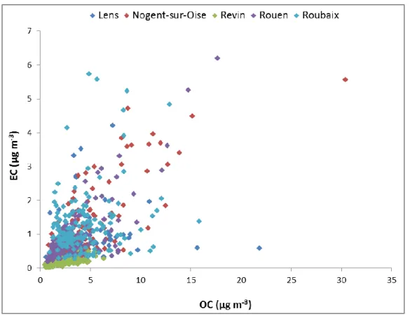
(14) Thèse de Diogo Miguel BARROS de OLIVEIRA, Lille 1, 2017. Figure 18: Geographical location of the sampling site in Rouen ............................................. 66 Figure 19: Meteorological data for the site of Rouen (temperature and rainfall in the left and windrose in the right) ............................................................................................................... 67 Figure 20: Meteorological data for the site of Revin (temperature and rainfall in the left and windrose in the right) ............................................................................................................... 68 Figure 21: Geographical location of the sampling site of Roubaix .......................................... 69 Figure 22: Meteorological data for the site of Roubaix (temperature and rainfall) ................. 69 Figure 23: High-volume sampler Digitel DA80 ...................................................................... 70 Figure 24: Scheme of the protocol to obtain uncertainties linked to measurements (source: Ellison et al. 2000) ................................................................................................................... 74 Figure 25: Uncertainties fishbone scheme for ICP measurements (source: Yenisoy-Karakaş 2012)......................................................................................................................................... 75 Figure 26: Uncertainties fishbone scheme for IC measurements (source: Leiva et al., 2012) . 76 Figure 27: Uncertainties fishbone scheme for metal measurements carried out in Mines Douai .................................................................................................................................................. 77 Figure 28: Balance between anions and cations on each sampling site ................................... 79 Figure 29: Correlation between anions and cations on all sampling sites (1:1 ratio) .............. 80 Figure 30: Seasonal variation of the ion balance on each sampling site .................................. 81 Figure 31: Difference between anions and cations on each sampling site per season ............. 83 Figure 32: Correlation between PM10 measurements and mass closure method ..................... 85 Figure 33: PM10 reconstructed mass and unaccounted fraction per season at each sampling site .................................................................................................................................................. 87 Figure 34: PM10 average concentration on each site per season .............................................. 90 Figure 35: Average chemical composition of PM10 on each sampling site ............................. 90 Figure 36: Average chloride per sodium ratio for each site according to their distance to the sea ............................................................................................................................................. 91 Figure 37: EC (top) and OC (bottom) average concentrations on each sampling site, per season ....................................................................................................................................... 92 Figure 38: Correlation between EC and OC on all sampling sites ........................................... 94 Figure 39: OC/EC ratio at each sampling site per season ........................................................ 95 Figure 40: Average contribution of the organic species measured on each sampling site ....... 96 Figure 41: Organic species concentrations on each sampling site, per season ........................ 98 Figure 42: Ion contribution to PM10 mass on each sampling site .......................................... 101 Figure 43: Ion concentrations on each sampling site, per season .......................................... 102. © 2017 Tous droits réservés.. lilliad.univ-lille.fr.

(15) Thèse de Diogo Miguel BARROS de OLIVEIRA, Lille 1, 2017. Figure 44: Average contributions of the calculated species of NaCl, NaNO3, NH4NO3 and (NH4)2SO4 for each sampling site .......................................................................................... 104 Figure 45: Seasonal distribution of exceedance episodes on each site .................................. 105 Figure 46: Time distribution of exceedance episodes on each sampling site ........................ 106 Figure 47: Average chemical composition during exceedance episodes on each sampling site ................................................................................................................................................ 107 Figure 48: Chemical composition of the samples of March 30, 2013 at all sites, except Nogent-sur-Oise sampled on the 29th ..................................................................................... 108 Figure 49: Chemical composition of the samples of March 6, 2013 to all sites .................... 109 Figure 50: Qtrue/Qexp values for different number of factors in Nogent-sur-Oise............... 172 Figure 51: IM and IS values for different number of factors in Nogent-sur-Oise ................. 172 Figure 52: ZeFir interface for wind (top) and trajectory (bottom) calculations ..................... 174 Figure 53: Correlations between wood smoke concentrations obtained from levoglucosan and biomass burning contributions calculated from PMF on each sampling site ......................... 233 Figure 54 & 55: Primary traffic (top) and biomass burning (bottom) average and seasonal contributions in µg m-3 ........................................................................................................... 235 Figure 56 & 57: Land biogenic (top) and marine biogenic (bottom) average and seasonal contributions in µg m-3 ........................................................................................................... 236 Figure 58 & 59: Fresh marine (top) and aged marine (bottom) average and seasonal contributions in µg m-3 ........................................................................................................... 237 Figure 60, 61 & 62: Nitrate rich (top), sulfate rich (middle) and oxalate rich (bottom) average and seasonal contributions in µg m-3 ...................................................................................... 238 Figure 63: Average source contribution during days with PM10 mass concentration above 50 µg m-3 in Lens, Nogent-sur-Oise, Revin, Rouen and Roubaix .............................................. 240 Figure 64: Average source contribution during the 6th of March of 2013 in Lens, Nogent-surOise, Revin, Rouen and Roubaix ........................................................................................... 241 Figure 65: Average source contribution during the 30th of March of 2013 in Lens, Nogent-surOise, Revin, Rouen and Roubaix ........................................................................................... 242 Figure 66: Regional and local (top) and natural and anthropogenic sources (bottom) average contributions on the urban sites (Lens, Nogent-sur-Oise and Rouen) ................................... 243 Figure 67: Regional and local (left) and natural and anthropogenic sources (right) average contributions on the traffic site (Roubaix) ............................................................................. 244 Figure 68: Regional and local (left) and natural and anthropogenic sources (right) average contributions on the remote site (Revin) ................................................................................ 245. © 2017 Tous droits réservés.. lilliad.univ-lille.fr.

(16) Thèse de Diogo Miguel BARROS de OLIVEIRA, Lille 1, 2017. Figure 69: Average contribution of the different sources to PM10 mass concentration in Lens in Oliveira et al (left) and Waked et al (right) ........................................................................ 247 Figure 70: Relative contribution of Natural, Anthropogenic and Mixed sources to PM10 mass concentration in 6 sites in the north of France ....................................................................... 249 Figure 71: Relative contribution of marine sources to PM10 mass concentration in 6 sites in the north of France ................................................................................................................. 250 Figure 72: Relative contribution of Natural, Anthropogenic and Mixed sources to PM10 mass concentration in 5 European cities ......................................................................................... 252 Figure 73: Relative contribution of Natural, Anthropogenic and Mixed sources to PM10 mass concentration in 9 sites spread across the north of France and Belgium ............................... 253. © 2017 Tous droits réservés.. lilliad.univ-lille.fr.

(17) Thèse de Diogo Miguel BARROS de OLIVEIRA, Lille 1, 2017. LIST OF TABLES Table 1: Main anthropogenic sources of metals in atmospheric particles (source: Riffault et al. 2015)......................................................................................................................................... 37 Table 2: WHO database on local source apportionment studies of particulate matter in air. The studies performed with PMF are highlighted in green (source: WHO) ................................... 48 Table 3: Comparison of the meteorological conditions between the winter of 2013 and the winter of 2014 .......................................................................................................................... 82 Table 4: OM/OC ratio used in each sampling site ................................................................... 84 Table 5: Unaccounted masses for each sampling site .............................................................. 84 Table 6: Number of samples for each sampling site - total and per season ............................. 88 Table 7: Validated (checked) species used at each sampling site ............................................ 89 Table 8: EC and OC average concentrations and standard deviations (µgC m-3) at each sampling site, per season .......................................................................................................... 93 Table 9: Between site correlation coefficients for levoglucosan contributions during the studied period from the 5 sites ................................................................................................. 99 Table 10: Average and seasonal ratios of L/M and L/(M+G) for each sampling site ............ 100 Table 11: Number of exceedance episodes on each site, during the sampling period ........... 105 Table 12: MeteoFrance stations used for each sampling and their corresponding distance .. 231 Table 13: Contributions to PM10 mass of wood smoke (calculated from levoglucosan by a factor of 10.7), biomass burning factors (obtained from PMF) and the new calculated factor ................................................................................................................................................ 232. © 2017 Tous droits réservés.. lilliad.univ-lille.fr.


(19) Thèse de Diogo Miguel BARROS de OLIVEIRA, Lille 1, 2017. GENERAL INTRODUCTION. © 2017 Tous droits réservés.. lilliad.univ-lille.fr.


(21) Thèse de Diogo Miguel BARROS de OLIVEIRA, Lille 1, 2017. GENERAL INTRODUCTION Air quality is a major environmental, social and economical issue in this day and age. It is a complex problematic hard to manage and mitigate, and has been proven to be the largest environmental health risk in Europe (WHO, 2016). Although particulate matter (PM), also commonly referred to as ‘aerosols’, is present naturally in the atmosphere, its number greatly increased with the Industrial Revolution in the end of the 19th century due to anthropogenic activities. However, just in 1980 the first legislation concerning PM limit values was put in place in Europe with the Directive 80/779/EEC (Kuklinska, Wolska, and Namiesnik 2015). In order to control and reduce PM emissions it became crucial to understand the nature and sources of these particles in the atmosphere. PM can then be distinguished by being from natural origin (marine sea salt, biogenic particles, crustal matter from soil erosion, volcanic activity, wild fires, etc.) or anthropogenic origin (industrial activity, processes of fossil fuel combustion, agriculture, traffic, etc.). The nature of the aerosols is directly related with their impact on human health with several studies reporting links between PM chemistry and respiratory and cerebrovascular diseases (Anderson, Thundiyil, and Stolbach 2012), heart disease (Pope III and Dockery 2006) and even carcinogenic potential (Sun et al. 2004; Giakoumi et al. 2009). Driven by evidence of the ill effects of PM to human health, a limit value of 40 µg m -3 of PM10 as an annual average is now imposed in the European Union by the Air Quality Directive 2008/50/EC. A limit daily average value of 50 µg m-3 is also imposed and it shouldn’t be exceeded more than 35 days in one year. These limits encourage local governments to invest on the knowledge of these particles and their sources in order to reduce its values. PM can also be characterized as primary or secondary particles. Primary particles are emitted directly to the atmosphere. Secondary particles are formed in the atmosphere from chemical or photochemical reactions and/or physical modification. These secondary particles are associated with precursor gases like sulfur dioxide, NOx (nitrogen oxide and nitrogen dioxide), ammonia or volatile organic compounds. The dispersion, transport and deposition of these particles are key parameters to understand the impact of air pollution not only on a local scale but also on regional and global scale. Starting by the latter, deposition of aerosols can occur by dry deposition (gravity effect 21. © 2017 Tous droits réservés.. lilliad.univ-lille.fr.

(22) Thèse de Diogo Miguel BARROS de OLIVEIRA, Lille 1, 2017. (Sehmel 1980)) or by wet deposition (particles may either serve as condensation nuclei for droplet formation or they collide with droplets either within or below clouds (Seinfeld and Pandis 2006). Dispersion and transport are linked with meteorological conditions and particles properties, where the first also depends on emission patterns. Although PM10 levels have been gradually decreasing over the last 10 years, the constant urban growth of developed and developing countries poses major concerns in terms of the impact of air pollution in citizens. In fact, the exceedance of the daily limit value of PM10 mentioned above was observed in 22 Member States of the EU at one or more stations in the year of 2015. A stricter value of 20 µg m-3 is suggested by the World Health Organization (WHO) and this was exceeded at 67% of the stations and in 27 European countries, according to the “Air Quality in Europe” report (EEA, 2016). In France, where an estimated 42 000 premature deaths per year occur due to air pollution exposure, PM10 is monitored in over 338 stations, most of them inserted in urban environments (~60%), some in close distance to intense traffic activity (~20%) and in rural areas (~7%). Just 4 of these stations exceeded the annual limit value for PM10 levels in 2013 (all in traffic sites), however 12% of all the stations recorded more than 35 days where the average daily value was exceeded, mostly urban and traffic stations. In fact, PM10 levels in France have barely decreased during the last 5 years, and 8 of the 41 largest metropolitan areas (over 250k inhabitants) exceeded PM10 daily limit values (LCSQA, 2016). The north of France in particular is characterized by short but frequent pollution episodes. In fact, a study from LCSQA identified the Nord-Pas de Calais region as one of the most polluted in France, where about 90% of its population was exposed to more than 35 daily exceedance episodes in the year of 2007. Although the average annual value is below the EU limit (24 µg m-3 in 2014) it is still above the one recommended by the WHO, and the number of daily exceedance episodes is concerning (over 35 in 6 urban areas). To understand and better tackle this issue, information on all these aspects needs to be gathered and measures on the controllable parameters have to be put in place. This requires to assess what are exactly the sources of PM on a given place/region, and to do so several mathematical methods of data treatment are put in place. This work will be based on the ones that are receptor-oriented, meaning that PM is collected at a given sampling site, characterized and this information is used to calculate its probable sources. Based on observations on. 22. © 2017 Tous droits réservés.. lilliad.univ-lille.fr.

(23) Thèse de Diogo Miguel BARROS de OLIVEIRA, Lille 1, 2017. chemical speciation, our approach will aim at apportioning and locating source of PM impacting the north of France. This document will start with a first chapter dedicated to the state of art in order to introduce the main issues and present the objectives and approaches of this work. A second part will present the material and methods used during this work, with a first presentation of the results obtained for the chemical characterization of the samples collected. A third chapter, based on a publication already submitted, aims to present the methodology used on a full source apportionment study on a single sampling site in the north of France. Finally a fourth chapter based on a publication as well, will present the main results of a multi-site approach of the methodology suggested in chapter 3. This manuscript ends with the conclusion where the summary of the main results will be provided and with the suggestion of some perspectives for future improvements.. 23. © 2017 Tous droits réservés.. lilliad.univ-lille.fr.

(24) Thèse de Diogo Miguel BARROS de OLIVEIRA, Lille 1, 2017. 24. © 2017 Tous droits réservés.. lilliad.univ-lille.fr.

(25) Thèse de Diogo Miguel BARROS de OLIVEIRA, Lille 1, 2017. CHAPTER 1 BIBLIOGRAPHY ON COMPOSITION AND SOURCES OF TROPOSPHERIC AEROSOLS. 25. © 2017 Tous droits réservés.. lilliad.univ-lille.fr.


(27) Thèse de Diogo Miguel BARROS de OLIVEIRA, Lille 1, 2017. CHAPTER 1 - BIBLIOGRAPHY ON COMPOSITION AND SOURCES OF TROPOSPHERIC AEROSOLS. 1.1. Particulate matter. Particulate matter (PM) is a mixture of solid or liquid particles suspended in air. PM, also commonly referred as “aerosols”, is found in the atmosphere with a multitude of shapes and sizes, originated from wide range of sources which are important characteristics that will determine the lifetime of these particles in the atmosphere. Spanning from a few hours to a few weeks, the lifetime of aerosols (and their link to very specific sources) explains the highly non-uniform distribution of concentrations seen around the globe. In direct relation, the size distribution of PM can range from hundreds of micrometers down to just a few nanometers and it can be used to categorize aerosols by different size modes and relate them with specific sources, chemistry and removal processes. To do so, one can use the aerodynamic diameter of PM as physical property to characterize size modes. Aerodynamic diameter is defined for an irregularly shaped particle in terms of the diameter of an ideal spherical particle of unit density that has an aerodynamic behavior identical to that of the particle in question (Hinds 1982). Based on the equality of their settling velocities, equation 1 gives the relationship between the characteristics of a real particle (effective diameter, particle density, shape coefficient) and its aerodynamic diameter: 𝜌𝑝. 𝑑𝑎 = 𝑑𝑒 ∙ √𝜌. 0 ∙𝜒. da de p 0 . (Eq. 1). aerodynamic diameter of a sphere of unit density (µm) effective diameter of the real particle (µm) real particle density (g cm-3) unit density (1 g cm-3) shape coefficient of the real particle ( of a sphere equals to 1). According to the International Standards Organization (ISO), PM10 is defined as particles which pass through a size-selective inlet with a 50 % efficiency cut-off at 10 μm aerodynamic diameter. PM10 is therefore a standard size fraction where the median diameter is 10 microns. Similarly with other size fractions, 50% of the PMx have a diameter greater than x microns (Seinfeld and Pandis 2006). 27. © 2017 Tous droits réservés.. lilliad.univ-lille.fr.

(28) Thèse de Diogo Miguel BARROS de OLIVEIRA, Lille 1, 2017. 1.1.1. Sources of PM10. Atmospheric particles can be classified according to their origin. This term can however encompass different meanings, that is to say geographical origin, emitting source or formation process. Before discussing the sources of particles, it is necessary to distinguish between primary and secondary aerosols. Primary aerosols are directly released as particles in the atmosphere. On the other hand, secondary aerosols are formed by gas-to-particle conversion processes from semi-volatile gaseous species or precursor gases through physical or chemical processes. Concerning sources of particles or their gaseous precursors, two main origins can be distinguished in the atmosphere: natural and anthropogenic sources. 1.1.1.1. Natural sources. The main natural primary aerosols are sea salt particles with contributions that can range from 10% up to 60% (Carslaw et al. 2010), and on average sea spray accounts for half of the natural PM10 (IPCC, 2013) – about 4100 Tg yr-1, which are emitted from the oceans by evaporated sea spray. Mineral dust, originating from arid and semi-arid regions of the world (mainly Saharan and Gobi deserts), is the second important contributor of natural primary particles on average – 2500 Tg yr-1 (IPCC, 2013) and the main contributor in continental regions like South Asia and China. Because mineral desert dust can be transported over thousands of kilometers, it has a global impact. The chemical composition of mineral particles is highly variable and depends on the source region and transport pathways. The main constituents are silicon oxides (SiO2), carbonates like calcite (CaCO3) and dolomite (CaMg(CO3)2), sulfates, phosphates and iron oxides like hematite (Trochkine et al. 2003). Volcanic dust and biogenic particles (e.g. pollens) are other natural primary particles. All these natural primary particles are mainly found in the coarse mode (i.e. over 2.5 µm) of the aerosol size distribution (see figure 1). Typical natural sources of secondary aerosols are the biosphere and volcanoes that emit sulfur (e.g. in form of dimethyl sulfide, DMS, and sulfur dioxide into the atmosphere) which can be oxidized to sulfate and form sulfuric acid nuclei. These nuclei may then coagulate and grow by water uptake to form small droplets in the accumulation mode. The biosphere can also emit volatile organic compounds (VOCs) that can be oxidized and form new particles, with emissions ranging from 20 up to 380 Tg yr-1 (IPCC, 2013; Kanakidou et al. 2005).. 28. © 2017 Tous droits réservés.. lilliad.univ-lille.fr.

(29) Thèse de Diogo Miguel BARROS de OLIVEIRA, Lille 1, 2017. Figure 1: Principal modes, sources, and particle formation and removal mechanisms shown for an idealized aerosol surface size distribution (Zieger 2011). 1.1.1.2. Anthropogenic sources. Anthropogenic emissions of primary particles include black carbon (ranging from 3.6 up to 6 Tg yr-1, averaging 4.8 Tg yr-1 around the globe, according to the IPCC report (2013)) from incomplete combustion and organic matter, which can be the main contributor of anthropogenic emissions in urban areas in the American continent – 20% or more, or around 16% in other regions being the second or third contributor (IPCC, 2013). Dust emissions, although still ill quantified, also have a significant anthropogenic component mainly originating from agricultural and industrial processes and road traffic, with contributions of 20% to 25% of the PM (Ginoux et al. 2012). Secondary aerosol sources of anthropogenic 29. © 2017 Tous droits réservés.. lilliad.univ-lille.fr.

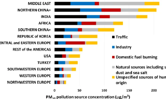
(30) Thèse de Diogo Miguel BARROS de OLIVEIRA, Lille 1, 2017. origin include sulfates from SO2, nitrates from NOx and ammonium from ammonia emissions, as well as biomass burning and organics from anthropogenic VOCs. These gases can be emitted, for example, through domestic heating systems based on coal or wood combustion, industrial plants, vehicle emissions and agricultural activities. Although the global emissions are dominated by the natural sources, Seinfeld and Pandis (2006) give an estimate of 3100 Tg yr-1, and more recently IPCC (2013) ranged this emissions from 2920 up to 13000 Tg yr-1, they are mainly related to contributions from the coarse mode, while the emissions from anthropogenic sources (Seinfeld and Pandis, 2006, estimate 450 Tg yr-1) are mainly contributions from the fine mode (with correspondingly higher number concentration). However anthropogenic emissions are mostly seen either in highly populated areas either near them, having a direct effect on inhabitants of these regions.. 1.1.2. PM10 composition. As mentioned above regarding the main origins of tropospheric aerosols, PM can be classified as primary or secondary aerosols, as previously mentioned. From an analytical point of view, they can also be mentioned as organic or inorganic aerosols. The IPCC report of 2013 on air quality compiled studies where PM was sampled and chemically analyzed, identifying the major components to its mass and their dependence with site typology and region of the world (figure 2).. 30. © 2017 Tous droits réservés.. lilliad.univ-lille.fr.

(31) Thèse de Diogo Miguel BARROS de OLIVEIRA, Lille 1, 2017. Figure 2: Bar chart plots summarizing the mass concentration (μg m–3) of seven major aerosol components for particles with diameter smaller than 10 μm, from various rural and urban sites (dots on the central world map) in six continental areas of the world with at least an entire year of data and two marine sites (IPCC, 2013). 1.1.2.1. Carbonaceous aerosols. The organic fraction represents a major component of PM, contributing between 20 and 80% of the total mass of PM in urban and industrialized areas (Cheung et al. 2011; Jacobson 2002; Nunes and Pio 1993; Stone et al. 2010). Organic matter (OM) or organic aerosols (OA) can be emitted directly into the atmosphere in the form of particles (POA), or can be formed in the atmosphere due to oxidation reactions of volatile organic compounds (VOCs) followed by gas-particle conversion processes (Seinfeld and Pandis, 2006) forming secondary organic aerosols (SOA). OM mass is not measured directly, but can be estimated by multiplying the measured organic carbon by a determined factor (OM = OC × α) to take into account the level 31. © 2017 Tous droits réservés.. lilliad.univ-lille.fr.

(32) Thèse de Diogo Miguel BARROS de OLIVEIRA, Lille 1, 2017. of organic carbon functionalization in the particle (mass of hydrogen and hetero-atoms). This factor has been first estimated by White and Roberts (1977), calculating a ratio of 1.4 for specific organic compounds measured in Los Angeles (USA). Later, Turpin and Lim (2001) concluded that this ratio should be higher than 1.4 and around 1.6 for more urban areas, whereas 1.9–2.3 were suggested for aged aerosols. Unfortunately, there are only a very few experimentally derived conversion factors reported. The main sources of POA are biomass burning, fossil fuel combustion (industry, domestic, traffic), and wind-driven or traffic-related suspension of soil and road dust, biological materials (plant and animal debris, microorganisms, pollen, spores, etc.), and spray from the sea or other water surfaces with dissolved organic compounds (O’Dowd et al. 2004). SOA is formed by chemical reaction and gas-to-particle conversion of volatile precursors within the atmosphere. The SOA precursors can be both anthropogenic and biogenic. Current knowledge of precursor emissions and the aerosol formation potential of the individual precursors suggest that SOA formation from biogenic precursors dominates (Andersson-Sköld and Simpson 2001; Mattias Hallquist et al. 2009). Elemental carbon (EC) is actually a mixture of graphite-like particles and light-absorbing organic matter. Moreover, the surface of EC particles contains numerous adsorption sites that are capable of enhancing catalytic processes (Cao et al. 2004). As the result of its catalytic properties, EC may intervene in some important chemical reactions involving atmospheric sulfur dioxide (SO2), nitrogen oxides (NOx), ozone (O3) and other gaseous compounds (Gundel et al. 1984). On the atmosphere EC is primarily emitted from combustion processes related with anthropogenic activities, such as fossil fuel combustion and biomass burning as house heating method, and naturally also from biomass burning but associated with wild fires. On urban environments, EC is associated with anthropogenic like traffic emissions associated both with exhaust emissions – diesel soot – and non-exhaust emissions – abrasion of tire wearing. 1.1.2.2. Organic tracers. OM contains numerous organic species, including alkanes, alcohols, carboxylic acids, carbonyl compounds, and aromatic compounds, some of which can be used as source, transport, or receptor tracers in conjunction with volatile and inorganic species (B. R. T. Simoneit 1984; B. R. T. Simoneit 1989; Rogge et al. 1996; Schauer et al. 1996). Is then 32. © 2017 Tous droits réservés.. lilliad.univ-lille.fr.

(33) Thèse de Diogo Miguel BARROS de OLIVEIRA, Lille 1, 2017. interesting to understand not only the chemistry associated with PM but also the close connection with between specific species and sources: . Alkanes (CnH2n+2) Particulate n-alkanes have been determined in vehicle exhaust (Rogge et al. 1993; Schauer et al. 1999; Schauer et al. 2002), tire abrasion, brake lining dust as well as in road dust (Rogge et al., 1993). They are emitted in natural gas combustion (Rogge et al., 1993), from boilers (Rogge et al. 1997), and are contained in smoke from coal combustion (Oros and Simoneit 2000). The smoke of wood and synthetic logs burning is another source of particulate n-alkanes (Rogge et al. 1998; Schauer et al. 2001; Didyk et al. 2000; Fine, Cass, and Simoneit 2001; Fine, Cass, and Simoneit 2002). A carbon preference index (CPI) has also been commonly used to quantify the relative abundance of odd versus even-numbered carbon chain n-alkanes. It is a key diagnostic parameter in tracking the origin of organic inputs to determine the biogenic and anthropogenic nature of n-alkane sources (Pietrogrande et al. 2010). In particular, anthropogenic emissions from utilization of fossil fuel generate a random distribution of odd vs even terms yielding CPI values close to 1. On the other hand, hydrocarbons originated from terrestrial plant material show a predominance of odd-numbered terms showing CPI ≈ 5-10 (Cheng et al. 2006; Bi et al. 2005; Cincinelli et al. 2007).. . Anhydrosugars Anhydrosugars (levoglucosan mannosan, galactosan) are derived from pyrolysis of cellulose and hemicellulose at high temperatures (>300°C) (B. R. Simoneit et al. 1999). They are better molecular tracers of biomass burning aerosols compared to traditional tracers (e.g. K+ and BC) because of their single source (figure 3). Levoglucosan presents the higher concentrations. Although it can be degraded in the atmosphere, especially oxidized by OH radicals as reported in some simulation experiments and model studies (M. Hallquist et al. 2009; Hennigan et al. 2010), it is still considered as an ideal tracer for biomass burning due to its relative stability and high emission factors. Levoglucosan has been widely used as a tracer of biomass burning aerosols in many studies in continental and coastal regions (Fraser and Lakshmanan 2000; Xiaolei Zhang, Yang, and Blasiak 2012; Fine, Cass, and Simoneit 2002; Giannoni et al. 2012; T. Zhang et al. 2008; Sang et al. 2011; Křŭmal et al. 2010; X. Zhang et al. 2010). 33. © 2017 Tous droits réservés.. lilliad.univ-lille.fr.

(34) Thèse de Diogo Miguel BARROS de OLIVEIRA, Lille 1, 2017. Figure 3: Relative mass concentration of anhydrosugars in PM per source category (adapted from Pernigotti, Belis, and Spanò, 2016). . Monosaccharides and Polysaccharides Polysaccharides are complex carbohydrates (sugars), composed of 10 up to several thousand monosaccharides arranged in chains. Monosaccharides like glucose, mannose and galactose are aldohexoses and can form six-membered rings. These compounds are important thermal degradation products of cellulose, and therefore used as tracers for biomass burning activities (Saffari et al. 2013). Also, B. R. Simoneit et al. (2004) suggested that monosaccharides can also be tracers of soil material and associated with microbiota, adding as possible sources other anthropogenic activities like ploughing during agricultural activities (K. E. Yttri et al. 2007). The same study also showed a close relation between the emission of these sugars and ruptured pollen emitted during late spring and early summer, later confirmed by (P. Q. Fu et al. 2012).. . Sugar alcohols Sugar alcohols are polyols in which the aldose or ketose forms get hydrogenated, keeping the same linear structure as in monosaccharides but with the aldehyde (-CHO) group replaced by an alcohol -CH2OH group in each unit. Recently, Bauer et al. (2008) suggested that mannitol and arabitol concentrations are correlated with the fungal spore counts in atmospheric PM10. This finding was confirmed by X. Zhang et al. (2010) who measured arabitol and mannitol during April and May 2004 in southern China. These sugar alcohols are common storage substances in fungal spores. Bauer et al. (2008) suggest that using these polyols for spores simplifies sampling, analytical 34. © 2017 Tous droits réservés.. lilliad.univ-lille.fr.

(35) Thèse de Diogo Miguel BARROS de OLIVEIRA, Lille 1, 2017. analysis and evades the need for parallel aerosol collection. Mannitol, although common in fungi, is also a common sugar alcohol in plants; it is particularly abundant in algae and has been detected in at least 70 higher plant families. . Oxalate Oxalic acid is the dominant dicarboxylic acid (DCA) in atmospheric PM followed by malonic and succinic acids (Kawamura and Ikushima 1993; Kawamura and Usukura 1993; Yao et al. 2002; Yao, Fang, and Chan 2002), and it constitutes up to 50 - 70% of total atmospheric DCA (Sempére and Kawamura 1994; Sempéré and Kawamura 1996). Main sources of oxalic acid are thought to be photochemical oxidation of anthropogenic, biogenic and oceanic emissions and/or primary traffic emissions (Kawamura and Kaplan 1987; Kawamura, Kasukabe, and Barrie 1996). Very high concentrations of oxalic acid were detected in biomass burning plumes, suggesting that either oxalic acid is directly emitted or formed in the plume from a biogenic precursor (Jaffrezo, Calas, and Bouchet 1998). Oxalic acid is likely an end-product of the photochemical oxidation reactions and can accumulate in the atmosphere (Chebbi and Carlier 1996; Kawamura and Ikushima 1993). Once formed, it is expected to be very stable and to exist as fine particles. Hence, the major removal mechanism is expected to be wet deposition.. 1.1.2.3. Inorganic PM. The inorganic fraction includes mainly the ionic species sulfate (SO42-), nitrate (NO3-) and ammonium (NH4+). Although these species are predominantly from secondary origin, they may also be directly emitted from primary sources such as ship engines (Agrawal et al., 2008) and sea salt (ssSO42-). This inorganic water-soluble fraction is generally present in the fine PM fraction as ammonium sulfate ((NH4)2SO4), and ammonium nitrate (NH4NO3), and are formed in the atmosphere from gaseous precursors, such as ammonia (NH3), nitric acid (HNO3), and sulfuric acid (H2SO4) (Seinfeld and Pandis, 2006). Ammonium nitrate is characterized by its semi-volatility and its presence in the particulate phase depends both on weather conditions and concentrations of its gaseous precursors (NOx and NH3). According to emission inventories, the sources of NH3 are almost exclusively related to agriculture (livestock, fertilizer use). The major identified sources of ammonia include excreta. 35. © 2017 Tous droits réservés.. lilliad.univ-lille.fr.

(36) Thèse de Diogo Miguel BARROS de OLIVEIRA, Lille 1, 2017. from domestic and wild animals, synthetic fertilizers, oceans, biomass burning, crops, human populations and pets, soils, industrial processes and fossil fuels (Bouwman et al. 1997). HNO3 is formed in the atmosphere from the oxidation of nitrogen oxides (NO and NO2), emitted during combustion processes (biomass burning, combustion of fossil fuel) and lightning (S. E. Bauer et al. 2007). Sulfuric acid is formed from oxidation reactions in the gas or aqueous phases, involving SO2 emitted directly into the atmosphere by fossil fuels rich in sulfur (oil, coal) and by volcanic activity, or by other sulfur-rich VOCs such as DMS (dimethyl sulfide) emitted by marine sources (Seinfeld and Pandis, 2006). 1.1.2.4. Inorganic tracers. Among the inorganic components of PM, metals are often used as markers of various sources (table 1), which can be found in different size fractions ranging from below 0.01 to 100 μm and larger. Metals such as As, Au, Cd, Co, Cr, Cu, Eu, Fe, Ga, Ni, Mn, Mo, Pb, Se, Sb, V, W, and Zn exist in both the coarse and fine fractions in ambient air. Al, Ca, La, Hf, Mg, Sc, Th, and Ti exist predominantly in the coarse fraction. Metals such as Ba, Cs and Se enrich the fine fraction of PM. The toxic metals arsenic (As), cadmium (Cd), lead (Pb), mercury (Hg) and nickel (Ni) are mainly emitted as a result of various industrial activities and the combustion of coal. In Europe, their concentrations in ambient air are monitored and regulated (4th Daughter Directive 2004/107/EC). Although the atmospheric concentrations of these metals are generally low, they still contribute to the deposition and build-up of heavy metal contents in soils, sediments and organisms. They bioaccumulate in the environment, causing a long-term poisoning of plants, animals and food chains (EEA, 2016).. 36. © 2017 Tous droits réservés.. lilliad.univ-lille.fr.

(37) Thèse de Diogo Miguel BARROS de OLIVEIRA, Lille 1, 2017. Table 1: Main anthropogenic sources of metals in atmospheric particles (source: Riffault et al. 2015). Sources Construction industry (building boards) Exhaust and non-exhaust emissions (combustion, brake/tire wear, etc) Industrial oil combustion (petrochemistry, refinery and power plants) Energy production. Metals Al, Fe, Mn, Si and Ti Ba, Br, Cd, Cr, Cu, Fe, Pb, Sb and Zn. La, Ni and V As, Bi, Cd and Hg. Coal combustion. Al, As, Co, Cr, Cu and Se. Metallurgy (steel and non-steel industry). As, Cu, Fe, Mn, Ni and Pb. Waste incinerators. 1.2. Cd, Cu, Hg, K, Pb, Sb and Zn. Impacts and Regulation. The impact of aerosols on the atmosphere is widely acknowledged as one of the most significant and uncertain aspects of climate change projections. The observed global warming trend is considerably less than expected from the increase in greenhouse gases, and much of the difference can be explained by aerosol effects. There is also a growing concern for the impact of aerosols on human health and interest by many sectors such as weather prediction, the green energy industry (regarding their influence on solar energy reaching the ground) and the commercial aircraft industry and military (regarding the impact of PM on visibility and of volcanic ash and dust storms on operations and aircraft).. 1.2.1. Climate impact of PM. Aerosols play a significant role in the global energy balance and especially in atmospheric and surface energy balances regionally. A combination of surface direct radiative cooling, atmospheric warming through adiabatic heating, and indirect effects of aerosols on clouds, all contribute to the net aerosol effect. They are represented in modern climate models, yet their magnitudes are highly variable in space and time, and all are highly uncertain. The term “radiative forcing” has been employed in the IPCC Assessments to denote an externally imposed perturbation in the radiative energy budget of the Earth’s climate system. Such a perturbation can be brought about by secular changes in the concentrations of radiatively active species (e.g., CO2, aerosols), changes in the solar irradiance incident upon 37. © 2017 Tous droits réservés.. lilliad.univ-lille.fr.

(38) Thèse de Diogo Miguel BARROS de OLIVEIRA, Lille 1, 2017. the planet, or other changes that affect the radiative energy absorbed by the surface (e.g., changes in surface reflection properties). This imbalance in the radiation budget has the potential to lead to changes in climate parameters and thus to result in a new equilibrium state of the climate system. Anthropogenic aerosols scatter and absorb short-wave and long-wave radiations, thereby perturbing the energy budget of the Earth/atmosphere system and exerting a direct radiative forcing (figure 4).. Figure 4: Radiative forcing components (adapted from IPCC Fourth Assessment Report). Aerosols also serve as cloud condensation and ice nuclei, thereby modifying the microphysics, the radiative properties, and the lifetime of clouds. The aerosol indirect effect is usually split into two effects: the first indirect effect, whereby an increase in aerosols causes an increase in droplet concentration and a decrease in droplet size for fixed liquid water content (Twomey 1974); and the second indirect effect, whereby the reduction in cloud droplet size affects the precipitation efficiency, tending to increase the liquid water content, the cloud lifetime (Albrecht 1989), and the cloud thickness (Pincus and Baker 1994). Finally, it has been also reported a semi-indirect effect of aerosols on the energy budget of the atmosphere linked with the chemical nature of these particles. The presence of light absorbing 38. © 2017 Tous droits réservés.. lilliad.univ-lille.fr.

(39) Thèse de Diogo Miguel BARROS de OLIVEIRA, Lille 1, 2017. compounds (black and/or brown material) leads to an increase of cloud temperature. This increase in cloud temperature then leads to a consequent decrease on the relative humidity of the cloud and increase on the evaporation process of droplets (Lohmann and Feichter 2005).. 1.2.2. Health impact of PM. PM10 corresponds to the so-called “thoracic convention” (ISO 7708:1995, Clause 6). The 10 micrometer size does not represent a strict boundary between breathable and nonbreathable particles, but has been agreed upon for monitoring of airborne PM by most regulatory agencies. Particles larger than about 10 microns are mostly deposited higher up in the respiratory system and removed on the mucociliary escalator and may then be swallowed and subsequently absorbed through the gastro-intestinal tract. Many health effects of PM remain unknown and are estimated by epidemiological studies. These studies have shown a strong correlation between mortality and exposure to PM10 or PM2.5, the mortality being due to bronchial, heart disease or cancer (Analitis et al. 2006; Pope III and Dockery 2006). Indeed, the number of deaths from lung cancer due to exposure to PM2.5 represents approximately 11% of total lung cancer (AFSSET, 2005). Furthermore, PM exposure is also associated with the occurrence of diseases such as asthma, chronic bronchitis or chronic obstructive pulmonary disease (COPD) (Sunyer 2001; Liu et al. 2009). Indeed, it appears that a fraction of inhaled particles in the lung persists despite pulmonary clearance mechanisms (Churg et al. 2003). Moreover, the effects of PM are associated with their pulmonary penetrability, PM10 are deposited primarily in the upper alveolar regions while smaller particles penetrate to the airways (figure 5).. 39. © 2017 Tous droits réservés.. lilliad.univ-lille.fr.

(40) Thèse de Diogo Miguel BARROS de OLIVEIRA, Lille 1, 2017. Figure 5: Deposition of particles in the respiratory tract as a function of their size, with inset illustrating the proximity of the air spaces (alveoli) to the vasculature (in pink) (source: Elder, Vidyasagar, and DeLouise 2009). A recent study (Quan et al. 2010) indicates that PM2.5 leads to high plaque deposits in arteries, causing vascular inflammation and atherosclerosis — a hardening of the arteries that reduces elasticity, which can lead to heart attacks and other cardiovascular problems. Nawrot et al. (2011) concluded that traffic exhaust – being responsible of 7.4% of all heart attacks in the general public – is the single most serious preventable cause. Recent studies have shown the influence of PM on short-term morbidity and annual mortality. It was also seen that the toxicity of PM is driven by a complex interaction of size, location, source and season (Lippmann et al. 2013). PM exposure has also shown to have a small but significant adverse effect on cardiovascular, respiratory and cerebrovascular diseases (Anderson, Thundiyil, and Stolbach 2012). The link with specific aerosol sources is also important to understand the ill effects of anthropogenic activities and Kelly and Fussell (2015) suggested that a higher degree of toxicity is associated with traffic-related PM emissions both on fine and ultrafine fractions leading to increased morbidity and mortality from cardiovascular and respiratory conditions. Penetration of particles is not wholly dependent on their size; shape and chemical composition also play a part. A further complexity that is not entirely documented is how the shape of PM 40. © 2017 Tous droits réservés.. lilliad.univ-lille.fr.