Design Strategies for the Geometric Synthesis of Orthoglide-type Mechanisms

HAL Id: hal-00168494

https://hal.archives-ouvertes.fr/hal-00168494

Submitted on 28 Aug 2007

HAL is a multi-disciplinary open access

archive for the deposit and dissemination of sci-entific research documents, whether they are pub-lished or not. The documents may come from teaching and research institutions in France or abroad, or from public or private research centers.

L’archive ouverte pluridisciplinaire HAL, est destinée au dépôt et à la diffusion de documents scientifiques de niveau recherche, publiés ou non, émanant des établissements d’enseignement et de recherche français ou étrangers, des laboratoires publics ou privés.

Design Strategies for the Geometric Synthesis of

Orthoglide-type Mechanisms

Anatol Pashkevich, Philippe Wenger, Damien Chablat

To cite this version:

Anatol Pashkevich, Philippe Wenger, Damien Chablat. Design Strategies for the Geometric Synthesis of Orthoglide-type Mechanisms. Mechanism and Machine Theory, Elsevier, 2005, 40 (8), pp.907-930. �hal-00168494�

Design Strategies for the Geometric

Synthesis of Orthoglide-type Mechanisms

Pashkevich A.1, Wenger P.2 and Chablat D.2* 1

Belarusian State University of Informatics and Radioelectronics P. Brovka str, 220027 Minsk, Republic of Belarus

pap@bsuir.unibel.by

Tel. 375 17 239 86 73, Fax. 375 17 231 09 14 2

Institut de Recherche en Communications et Cybernétique de Nantes1 1, rue de la Noë B.P. 6597, 44321 Nantes Cedex 3, France

{Philippe.Wenger, Damien.Chablat}@irccyn.ec-nantes.fr Tel. 33 2 40 37 69 54, Fax. 33 2 40 37 69 30

A

BSTRACT

The paper addresses the geometric synthesis of Orthoglide-type mechanism, a family of 3-DOF parallel manipulators for rapid machining applications, which combine advantages of both serial mechanisms and parallel kinematic architectures. These manipulators possess quasi-isotropic kinematic performances and are made up of three actuated fixed prismatic joints, which are mutually orthogonal and connected to a mobile platform via three parallelogram chains. The platform moves in the Cartesian space with fixed orientation, similar to conventional XYZ-machine. Three strategies have been proposed to define the Orthoglide geometric parameters (manipulator link lengths and actuated joint limits) as functions of a cubic workspace size and dextrous properties expressed by bounds on the velocity transmission factors, manipulability or the Jacobian condition number. Low inertia and intrinsic stiffness have been set as additional design goals expressed by the minimal link length requirement. For each design strategy, analytical expressions for computing the Orthoglide parameters are proposed. It is showed that the proposed strategies yield Pareto-optimal solutions, which differ by the kinematic performances outside the prescribed Cartesian cube (but within the workspace bounded by the actuated joint limits). The proposed technique is illustrated with numerical examples for the Orthoglide prototype design.

1

IRCCyN: UMR n° 6597 CNRS, École Centrale de Nantes, Université de Nantes, École des Mines de Nantes

*

1.

INTRODUCTION

Parallel kinematic machines (PKM) are commonly claimed to offer several advantages over their serial counterparts, such as high structural rigidity, better payload-to-weight ratio, high dynamic capacities and high accuracy [1-3]. Thus, they are prudently considered as promising alternatives for high-speed machining and have gained essential attention of a number of companies and researchers. Since the first prototype presented in 1994 during the IMTS in Chicago by Gidding&Lewis (the VARIAX), many other parallel manipulators have appeared. However, most of the existing PKM still suffer from two major drawbacks, namely, a complex workspace and highly non-linear input/output relations [4, 5].

For most PKM, the Jacobian matrix, which relates the joint rates to the output velocities, is not isotropic. Consequently, the performances (e.g. maximum speeds, forces, accuracy and rigidity) vary considerably for different points in the Cartesian workspace and for different directions at one given point. This is a serious disadvantage for machining applications [6, 7], which require regular workspace shape and acceptable kinetostatic performances throughout. In milling applications, for instance, the machining conditions must remain constant along the whole tool path [8]. Nevertheless, in many research papers, this criterion is not taken into account in the algorithmic methods used for the optimization of the workspace volume [9, 10].

In contrast, for the conventional XYZ-machines, the tool motion in any direction is linearly related to the motions of the actuated axes. Also, the performances are constant throughout the Cartesian parallelepiped workspace. The only drawback is inherent to the serial arrangement of the links, which causes poor dynamic performances. So, in recent years, several new parallel kinematic structures have been proposed. In particular, a 3-dof translational mechanism with gliding foot points was found in three separate works to be fully isotropic throughout the Cartesian workspace [11-13]. Although this manipulator behaves like the conventional Cartesian mechanism, its legs are rather bulky to assure stiffness. The latter motivates further research in PKM architecture that seeks for compromise solutions, which admit a partial isotropy in favour of other manipulator features. One of such compromise solutions is the Orthoglide proposed by Wenger and Chablat[14], which was derived from a Delta-type architecture with three fixed linear joints and three articulated parallelograms. As follows from the previous works, this manipulator possesses good (almost isotropic) kinetostatic performances and also has some technological advantages, such as (i) symmetrical design; (ii) quasi-isotropic workspace; and (iii) low inertia effects [15]. In a previous

work, the Orthoglide was optimised with respect to the Jacobian matrix conditioning and transmission factor limits throughout a prescribed Cartesian workspace [16].

This paper further contributes to the Orthoglide kinematic synthesis and focuses on the comparison of different design strategies and inherited criteria. It proposes a systematic design procedure to define the manipulator geometric parameters (the actuated joint limits and the link lengths) as function of the prescribed cubic workspace size and performances measure bounds. The reminder of the paper is organized as follows. Section 2 briefly describes the Orthoglide kinematics and defines the design goals. Section 3 investigates the manipulator performances through the workspace. Section 4 deals with the design of the dextrous workspace with bounded manipulability, condition number and velocity transmission factors. Section 5 focuses on defining the largest cube inscribed in the dextrous workspace. Section 6 illustrates the proposed design strategies by numerical examples and also contains some discussions. And, finally, Section 7 summarises the main contributions of the paper.

2.

ORTHOGLIDE

KINEMATICS

AND

DESIGN

GOALS

2.1. M

ANIPULATOR GEOMETRY

The kinematic architecture of the Orthoglide is shown in Fig. 1. It consists of three identical parallel chains that may be formally described as PRPaR, where P, R and Pa denote the prismatic, revolute,

and parallelogram joints respectively. The mechanism input is made up of three actuated orthogonal prismatic joints. The output machinery (with a tool mounting flange) is connected to the prismatic joints through a set of three parallelograms, so that it is restricted for translational movements only.

Fig. 1. Kinematic architecture of the Orthoglide x y z (ρx, 0, 0) (0, ρy, 0) (0, 0, ρz) (px, py, pz) O (a) θz θx θy x y z O (b) ρx =L p=0 ρy =L ρz =L

Fig. 2. Orthoglide simplified model (a) and its “zero” configuration (b).

Because of its symmetrical structure, the Orthoglide can be presented in a simplified model, which consists of three bar links connected by spherical joints to the tool centre point at one side and to the corresponding prismatic joints at another side (Fig. 2a).

the x, y, z-axes are directed along them, the manipulator geometry may be described by the equations

(

)

2 _{2 2 2 2}

(

)

2 _{2 2 2 2}

(

)

2 ₂ ; ; x x y z x y y z x y z z p −ρ +p + p =L p + p −ρ +p =L p +p + p −ρ = (1) L

where p=

(

p p p_x, _y, _z

)

is the output position vector, ρ=

(

ρ ρ ρ_x, _y, _z

)

is the input vector of the prismatic joints variables, and L is the length of the parallelogram principal links. It should be noted that, for this convention, the “zero” position p₀ =

(

0, 0, 0

)

corresponds to the joints variables

(

L L L, ,

)

=

0

ρ , see Fig. 2b.

It is also worth mentioning that the Orthoglide geometry and relevant manufacturing technology impose the following constraints on the joint variables

0<ρ_x≤2L ; 0<ρ_y≤2L ; 0<ρ_z ≤2L, (2)

which essentially influence on the workspace shape. While the upper bound is implicit and obvious, the lower one is caused by practical reasons, since safe mechanical design encourages avoiding risk of simultaneous location of prismatic joints in the same point of the Cartesian workspace. Hence the kinematic synthesis must produce required joint limits within (2).

2.2. I

NVERSE KINEMATICS

From equations (1), the inverse kinematic relations can be derived in a straightforward way

2 2 2

x px sx L py pz

ρ = + − − ; ρ_y = p_y+s_y L2 −p_x2−p_z2 ; ρ_z = p_z+s L_z 2 −p_x2−p2_y (3) where s s sx, y, z∈ ±

{ }

1 are the configuration indices defined as signs of ρx− , px ρy− , py ρz−pz

respectively. Their geometrical meaning is illustrated by Fig. 2a, where θ θ θx, y, z are the angles

between the bar links and corresponding prismatic joint axes. It can be easily proved that s= +1 if

o o

(90 ,180 )

a

θ ∈ and s= −1 if θa∈(0 , 90 )o o , where the subscript a belongs to the set a∈

{

x y z, ,

}

. It should be also stressed that the border (θ =90o) corresponds to the serial singularity (when the link is orthogonal to the relevant translational axis and the input joint motion does not produce the end-point displacement), so corresponding Cartesian points must be excluded from the Orthoglide workspace during the design.

It is obvious that expressions (3) define eight different solutions to the inverse kinematics and their existence requires the workspace points to belong to a volume bounded by the intersection of three cylinders CL =

{

p px2+py2 ≤L2; px2+p2z ≤L2; py2+pz2 ≤L2

}

. However, the joint limits (2)

impose additional constraints, which reduce a potential solution set. For example, for the “zero” location p₀ =

(

0, 0, 0

)

, the equations (3) give eight solutions ρ =

(

± ±L, L,±L

)

but only one of them is feasible. As proved in [17], with respect to number of inverse kinematic solutions, the Orthoglide with joint limits (2) admits only 2 alternatives: (i) a single inverse kinematic solution

(s s s_x, _y, _z = + ) inside the sphere 1 S_L = ∈

{

p C_L p_x2+p_y2+ p_z2 <L2

}

; and (ii ) eight inverse kinematic solutions (s s s_x, _y, _z∈ ±

{ }

1 ) inside G_L =

{

p∈C_L |p p p_x, _y, _z >0; p_x2+p2_y+ p_z2 >L2

}

. It can be also proved that the border between these two cases corresponds to the serial singularity. Hence, the kinematic synthesis must focus on the location of the workspace inside of the sphere SL.

2.3. D

IRECT KINEMATICS

After subtracting three possible pairs of the equations (1) and analysis of the differences, the Cartesian coordinates px, py, pz can be expressed as

; ; 2 2 2 y x z x y z x y z t t t p ρ p ρ p ρ ρ ρ ρ = + = + = + , (4)

where t is an auxiliary scalar variable. This reduces the direct kinematics to the solution of a quadratic equation, At2+Bt C+ = with coefficients 0 A=

(

ρ ρ_{x y}

)

2+

(

ρ ρ_{x z}

)

2+

(

ρ ρ_{y z}

)

2;

(

)

2

x y z

B= ρ ρ ρ ;

(

2 2 2 2

)

(

)

2

4 4

x y z x y z

C= ρ +ρ +ρ − L ρ ρ ρ . The quadratic formula yields two solutions (2A)

) 4 ( B m B2 AC

t= − + − that differ by the configuration index m= ±1, which, from a geometrical point of view, distinguishes two possible locations of the target point with respect to the plane passing through the prismatic joint centres. Algebraically, this index can be defined as

(

1 1 1

)

sgn _{x x y y z z} 1

m= p ρ− +p ρ− + p ρ− − . It should be stressed that the case 2

4

B = AC corresponds to a parallel singularity, so corresponding joint coordinates must be excluded during the design.

It is obvious that the direct kinematic solution exists if and only if B2 ≥4AC, which defines a closed region in the joint variable space ℜ =_L

{

ρ|

(

ρ_x2+ρ2_y +ρ_z2−4L2

)(

ρ_x−2+ρ_y−2+ρ_z−2

)

≤1

}

. Taking into account (2), the feasible joint space may be presented as ℜ =+_L

{

ρ∈ℜ_L| ρ ρ ρ_x, _y, _z ≥0

}

. Hence, with respect to the number of direct kinematic solutions, the Orthoglide with joint limits (2) admits 2 alternatives [17]: (i) two direct kinematic solutions (m= ±1) inside the region ℜ ; and _L+ (ii) a single direct kinematic solution on the positive border of the region ℜ . Since the second case +_L corresponds to the singularity, the kinematic synthesis must focus on using the inner part of ℜ . _L+

2.4. D

ESIGN GOALS AND PARAMETERS

Because the Orthoglide is dedicated to general 3-axis machining, its kinematic performances should be close to the performances of the classical XYZ-machine. Therefore, the design goals may be stated as follows:

(i) manipulator workspace should be close to a cube of prescribed size; (ii) kinematic performances within this cube should be quasi-isotropic; (iii) link lengths should be minimal to lower the manufacturing costs.

The requirements (i) and (ii) will be satisfied in Section 4 by constraining the manipulability, condition number and/or velocity transmission factor inside the Cartesian workspace bounded by

the joint limits. To fulfil requirement (iii), Section 5 evaluates the largest cube inscribed in this workspace, which defines the smallest link lengths required to achieve the prescribed cube size. The design parameters to be optimised are the parallelogram length L, the actuated joint limits

)

(ρ_min,ρ_max and related location of the prescribed cube (p_min,p_max). Taking into account the linear relation between L and the workspace size, the design process is decomposed into two stages:

(i) defining the joint limits (ρ_min,ρ_max) and the largest cube size/location (p_min, p_max) to satisfy given kinematic performances for the normalised manipulator (L= ); 1

(ii) scaling the normalised manipulator parameters to achieve the prescribed size of the cubic workspace.

Numerical example for this two-stage design process is given in Section 6.

3.

JACOBIAN

ANALYSIS

3.1. J

ACOBIAN MATRIX

As follows from the previous Section and a companion paper [17], the singularity-free workspace of the Orthoglide W0 is located within the sphere SL of radius L with the centre point (0, 0, 0) and

bounded by the parallel “flat” singularity surface in the first octant (Fig. 3). Also, the remaining part of the sphere surface corresponds to the parallel “bar” singularity. Hence, the kinematic design should define the inner part of this workspace that possesses the desired kinematic properties.

Mathematically, these properties are defined by the manipulator Jacobian describing the differential mapping from the jointspace to the workspace (or vice versa). For the Orthoglide, it is more convenient to express analytically the inverse Jacobian, which is derived from (1) in a straightforward way: ⎥ ⎥ ⎥ ⎦ ⎤ ⎢ ⎢ ⎢ ⎣ ⎡ ρ ρ ρ ρ = − 1 ) /( ) /( ) /( 1 ) /( ) /( ) /( 1 ) , ( 1 z z y z z x y y z y y x x x z x x y -ρ p p -ρ p p -p p -p p -p p -p p ρ p J (5)

Accordingly, the determinant of the Jacobian may be expressed as

( )

1

₍

₎

₍

₎

₍

₎

det x y z x y z x y z x y z x x y y z z p p p p p p ρ ρ ρ ρ ρ ρ ρ ρ ρ ρ ρ ρ − ₌ + + − − − − J (6)

and admits two cases of ill-conditioning, det( )J =0 and det(J−1)=0, corresponding to the serial and parallel singularities mentioned above. It is also clear that the full isotropy is achieved only in the “zero” point p₀ =

(

0, 0, 0

)

, where the Jacobian reduces to the identity matrix: J₀ =I.

3.2. Q-

AXIS PROPERTIES

Since the Orthoglide workspace is symmetrical with respect to the axes x, y, z, its kinematic design requires a detailed study of the points belonging to the Q-axis, which is the bisector line of the first octant [16]. For this axis, let us denote p_x= = = and, consequently, p_y p_z p ρ ρ ρ ρ_x= = = . Then, as _{y z} follows from (5), the inverse Jacobian may be presented as

( )

⎥ ⎥ ⎥ ⎦ ⎤ ⎢ ⎢ ⎢ ⎣ ⎡ = − 1 1 1 1 χ χ χ χ χ χ χ J (7)

where χ is the dimensionless scalar parameter expressed as 2 2

2 p L

p −

− =

χ and related to the

input/output variables via the expressions p=−χL 1+2χ2 ; ρ =

(

1−χ

)

L 1+2χ2 . To define the feasible range of the parameter χ, let us consider specific points belonging to the Q-axis (see Fig. 4 and Table 1). They include three parallel singularity points P1, P2, P3 and one serial

singularity point P4. As follows from the analysis, the singularity-free region of the Q-axis is

bounded by the interval χ∈ −

(

0.5, 1.0

)

, which corresponds to the coordinate ranges

(

3 , 6

)

p∈ −L L ; ρ∈

(

0, 3 2 L

)

. It is important for the kinematic design that, within these limits, the relation between the coordinates p, ρ and the parameter χ is monotonously decreasing (see Table 1). It should be also noted that the employed parameterisation may be converted to the one used in [16] by defining χ = −tan( )θ , where θ is the angle between the manipulator links and corresponding prismatic joint axes.

px

py

pz _Q-axis

Fig. 3. The singularity-free workspace of the Orthoglide (97.2% of the sphere volume)

pz 2 2 y x p p r= + P2 P4 P1 P3 Q-axis Singularity-free workspace Q+ Q− O

Fig 4. Workspace regions for the Q-axis

Feature P1 O P2 P3 P4 p _{− 1 3} 0 _{1 6 1 3 1 2} ρ 0 1 _{3 2 4 3 1 2} χ 1 0 -0.5 -1 -∞

( )

det J ∞ 1 ∞ ∞ 0

4.

D

EXTERITY

-

BASED

D

ESIGN

Since the design specifications require the manipulator to possess the quasi-isotropic kinematics [18-20], the original joint limits (2) must be narrowed to increase the distance from the dextrous workspace points to the singularities. In this section, the desired joint limits are computed using the Q-axis technique, which reduces the problem to locating two points Q+ and Q-on the bisector line (see Fig. 4). These points bound the Q-axis region with the required properties and, therefore, define the joint limits. It is obvious that the interval [Q+, Q-] must include the fully-isotropic “zero” point O, and the kinematic performances at the points Q+, Q- should be similar. To compute the joint limits, we apply three different criteria evaluating the workspace dexterity. It should be also mentioned that all results of this Section are valid for the “unit” manipulator (L=1), which will be scaled on the subsequent design steps.

4.1. C

ONSTRAINING THE MANIPULABILITY

The manipulator manipulability w= det

(

J J−1 −T

)

is the simplest performance measure assessing the dexterity [21], which is the product of the singular values of the Jacobian or its inverse. For the Q-axis, where J−1 is a square and symmetrical matrix, the manipulability can be computed as

( )

₁

(

)

2

det 1 1 2

w= J− = −χ ⋅ + χ (8)

where χ∈ −

]

0.5, 1.0

[

. As follows from (6), the maximum value of the manipulability w is equal to 1 and is achieved in the “zero” (isotropic) point:

( )

(

1

)

0

det J− p =1; det

(

J−1

( )

p

)

<1 if p≠p₀ (9) Therefore, the joint limits can be found from the inequality

( )

(

1

)

min, max

det J− ρ ≥ Δ ∀ ∈ρ [ρ ρ ] , (10)

where Δ is the prescribed lower bound of the manipulability (Δ < ). Since the relation 1 ρ χ is

( )

monotonous and χ = corresponds to the isotropic posture (see sub-section 3.2), the desired 0 parameter range can be obtained from the cubic equation 2χ3−3χ2+ − Δ =

(

1

)

0 by selecting two roots closest to zero. Applying the trigonometric method, it can be obtained that

(

)

1 0.5 cos 3

χ = − ϕ , χ₂ =0.5 cos+

(

ϕ 3−π 3

)

, whereϕ =acos 1 2

(

− Δ

)

, χ₁<0, χ₂ >0, and, consequently, ρ_min =ρ χ

( )

₂ ; ρ_max =ρ χ

( )

₁ and p_min = p

( )

χ₂ ; p_max = p

( )

χ₁ , where functions ρ(χ) and p(χ) are defined in sub-section 3.2. The graphical interpretation of this result is presented in Fig. 5. The open question, however, is how to interpret the manipulability design specification Δ in engineering sense, to be understandable for the designer with a practical background.

χ1 χ2 det(J-1) = Δ Isotropic posture χ Manipulability 1.0 0.8 0.6 0.4 0.4 0 1.2

Joint limits ( |det(J-1)| > Δ )

1.2 1.0 0.8 0.6 0.4 0.2 1.4 0 -1.0 -0.5 0 0.5 1.0 1.5 0 0.2 0.4 0.6 0.8 1.0 |det(J-1)| ρ Isotropic posture 1.4 Δ ρmin ρmax det(J-1) = Δ

Fig. 5. Computing joint limits via the manipulability index.

4.2. C

ONSTRAINING THE CONDITION NUMBER

The Jacobian condition number evaluates the distance to the singularities by the ratio of the largest to the smallest matrix eigenvalues, which is also the ratio of the largest and smallest axis length of the manipulability ellipsoid [21]. As follows from (5), the Orthoglide condition number achieves its best value (equal to 1) in the zero point, while in other workspace points it is greater than 1:

(

( )

)

1

condJ-1 p₀ = cond

(

J-1(p)

)

>1 if p≠p₀ (11) Hence, the joint limits can be found from the inequality

(

1

)

min max

cond J− ( )ρ ≤δ ∀ ∈ρ ρ[ , ρ ], (12)

where δ is the admitted upper bound of this performance index (δ >1). Since along the Q-axis the inverse Jacobian is symmetrical, the condition number can be computed via the ratio of the largest to the smallest eigenvalues of J−1. The relevant characteristic equation det(J−1−λI)=0 may be rewritten as λ3−3λ2+3 1

(

−χ λ2

)

− −

(

1 χ

) (

2 2χ+ =1

)

0. Its analytical solution yields

1 1 2 ; 2,3 1

λ = + χ λ = − . Therefore, the condition number for the Q-axis can be expressed as χ

(

)

⎩ ⎨ ⎧ ∈ χ χ + χ − ∈ χ χ χ + = χ 0] 0.5, -] ) 2 (1 3 1 1[ 0, ] ) -(1 3 1 ) ( cond -1 if / if / J (13)

and the desired parameter range

[

χ χ can be obtained from the equations ₁, ₂

]

χ₁=−(δ-1)/(2δ+1), ) 2 ( ) 1 ( 2 = δ− δ+

χ / . Hence, ρ_min =ρ χ

( )

₂ ; ρ_max =ρ χ

( )

₁ and p_min = p

( )

χ₂ ; p_max = p

( )

χ₁ , where functions ρ(χ) and p(χ) are defined in sub-section 3.2. The graphical interpretation of this result is presented in Fig. 6. The question of defining a reasonable value of δ is simpler is this case because it possesses clearer geometric meaning and is rather understandable for practising engineers. Isotropic posture cond(J) = δ χ1 χ2 χ Inverse condition number

-1.0 -0.5 0.0 0.5 1.0 1.5 0 0.2 0.4 0.6 0.8 1.0 1.2 δ-1 ρmin ρmax

Joint limits ( cond(J) < δ ) 1.4 1.2 1.0 0.8 0.6 0.4 0.2 0 0 0.2 0.4 0.6 0.8 1.0 Isotropic posture cond(J) = δ cond(J)-1 ρ

Fig. 6. Computing joint limits via the condition number.

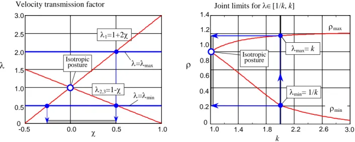
4.3. C

ONSTRAINING THE VELOCITY TRANSMISSION FACTOR

The velocity transmission factor assesses the ratio of the manipulator end-point velocity and velocity of the corresponding point in the joint space. For a given workspace point p and direction of motion e, it can be computed via the Jacobian as λ(p,e)=||J−1(p)⋅e||−1 where e eT =1. As known from the matrix theory, the deviation of this factor for the fixed p is bounded by the smallest

and largest singular values of J. Geometrically, this performance index is directly related to the

manipulability ellipsoid, which in the previous Sub-Section was evaluated by the ratio of its longest and shortest axes, while here these axes are assessed separately.

As follows from (5), the Orthoglide velocity transmission factor does not depend on the direction of motion in the zero point and in the remaining points it varies depending on e:

( )

( )

0

minλ , <1; maxλ , >1 if ≠

e p e e p e p p (14)

Hence, for this performance measure, the joint limits can be found from the inequality

( )

min , max [ min, max] , : 1

λ ≤λ ρ e ≤λ ∀ ∈ρ ρ ρ ∀e e = , (15)

where λ ρ

( )

,e denotes the velocity transmission factor along the Q-axis, and λmin, λmax are the

Since along the Q-axis the Jacobian is symmetrical, the transmission factor range may be derived from the eigenvalues obtained in the Sub-Section 4.2. It has been also proved that the eigenvalue

χ

λ₁ =1+2 corresponds to the eigenvector directed along the Q-axis, and two remaining coinciding eigenvalues λ_2,3 = 1−χ correspond to the eigenvectors, which are perpendicular to this axis. So, the desired parameter range

[

χ χ₁, ₂

]

can be computed from the expressions

(

)

{

}

1 max 1 max, min 1 / 2

χ = −λ λ − ; χ₂ =min 1

{

−λ_min,

(

λ_max−1 / 2

)

}

(16) Graphical interpretation of this result is presented in Fig. 7. The question of defining reasonable

values of λ_min, λ_max is very clear in this case. For instance λ∈

[

μ μ, 1

]

with μ∈

[

0.5, 1.0

]

possesses sensible meaning and is quite understandable for practising engineers. Impact of the transmission factor bounding on the dextrous workspace shape/size is also illustrated in Table 2, where all cases are quantified relative to the volume of the singularity-free workspace V0 (see

Fig. 3). To generate these shapes, we executed spanning of all possible directions from the isotropic point and dichotomic search for the line segments satisfying the kinematic constraints.

Isotropic posture λ=λmax λ=λmin λ1=1+2χ λ2,3=1-χ χ -0.5 0.0 0.5 1.0 0 0.5 1.0 1.5 2.0 2.5 3.0

Velocity transmission factor

λ k ρmin ρmax 1.4 1.2 1.0 0.8 0.6 0.4 0.2 0 1.0 1.4 1.8 2.2 2.6 3.0

Joint limits for λ∈[1/k, k]

Isotropic posture

λmax= k

ρ

λmin= 1/k

Fig. 7. Computing the joint limits the velocity transmission factors. Table 2

Dextrous workspace for different bounds on the velocity transmission factor

Lower bounding Two-sided bounding Upper bounding μ≥ 1/3 0.84·V0 μ∈ [1/3, 3] 0.67·V0 μ≤ 3 0.72·V0

μ≥ 1/2 0.51·V0 μ∈ [1/2, 2] 0.40·V0 μ≤ 2 0.52·V0

5.

W

ORKSPACE

-

BASED

D

ESIGN

After applying the Q-axis technique, which yields the joint limits ensuring the prescribed dexterity for the bisector line, the whole workspace must be verified for kinematic performances. In this Section, this problem is solved by identifying and evaluating the workspace “critical points” and relevant definition of the joint limits. Then, the largest cube is inscribed in the dextrous workspace of the unit manipulator, which gives the scaling factor to meet the specifications for the desired cubic workspace size. It should be noted that here the manipulator dexterity is evaluated by the velocity transmission factors, which, as stated above, have advantages over the manipulability and condition number indices in practical applications. But the main results are also generalised for the manipulability and condition number criterions.

5.1. W

ORKSPACE CRITICAL POINTS

Let us consider first the unit Orthoglide (L=1) with given joint limits ρ_min∈

[ ]

0, 1 , ρ_max∈ ⎣⎡1, 3 2⎤_⎦ and estimate the velocity transmission factors μ_min, μ_max over the corresponding workspace, which is bounded by six surfaces presented in Fig. 8. Since the manipulator has a symmetric geometric structure, the candidate points for extreme values of μ are located symmetrically on the workspace boundary and must be selected from the following sets:

(i) vertex points, for which all 3 joint coordinates ρ ρ ρ_x, _y, _z are equal to either ρ_min or ρ_max; (ii) edge points, for which 2 of 3 joint coordinates ρ ρ ρ_x, _y, _z are equal to either ρ_min or ρ_max; (iii) face points, for which 1 of 3 joint coordinates ρ ρ ρ_x, _y, _z is equal to either ρ_min or ρ_max; It is also obvious that the inner workspace points possess better dexterity than their boundary counterparts (since the straight line motion from the zero point to any boundary point causes monotonous changing of the angles θ θ θ_x, _y, _z and corresponding decreasing of the transmission factors for each axis). Besides, as follows from a detailed investigation, only three types of points, Q, R, and S, compete to define the global measure of the workspace performances. Hence, the problem of this Sub-Section is reduced to choosing the worst transmission factor from these points.

px py pz S+z z R+ z R− x S+ Q+ Q− z R− px py pz

Fig. 8. The ρ-bounded workspace and its critical points.

Vertex points Q+, Q−. For the points Q and Q+ −, which are located at the intersection of the workspace boundary and the bisector line (i.e. the Q-axis)

(

)

(

)

+

1 1 1 max max max

Q : p= p p p, , ; ρ= ρ ,ρ ,ρ ;

(

2 2 2

)

(

min min min

)

Q :− p= p p p, , ; ρ= ρ ,ρ ,ρ ;

the Jacobian is symmetrical, so the transmission factors μ_i are equal to the inverses 1λ1 and 2,3

1λ of the eigenvalues λ1 =1+2χ and λ2,3 = 1−χ (see Sub-Section 4.3). The parameter χ is

related to the Cartesian coordinates (p p p_x, _y, _z = ) by the expression p χ = −p 1 2− p2 , where p1,

p2 are expressed as

(

2

)

1 max max 1 3 2 3 p = ρ − − ρ ; ₂ 1

(

_min 3 2 _min2

)

3 p = ρ − − ρ (17) and corresponds to + Q and Q− respectively.

Edge points R_x+,...R . For the points _z− R_x+ and R_x−, which are defined at the intersection of the workspace boundary and the XY-plane

(

1 1

)

(

max max 1

)

: , , 0 ; , , x R+ p= p p ρ= ρ ρ ρ ;

(

2 2

)

(

min min 2

)

: , , 0 ; , , x R− p= p p ρ= ρ ρ ρ ;

the inverse Jacobian is

( )

1 2 2 1 0 1 0 1 1 1 χ χ χ χ χ χ χ − ⎡ ⎤ ⎢ ⎥ ⎢ ⎥ = ⎢ ⎥ − − ⎢ ⎥ ⎣ ⎦ J (18)

where χ =− p 1−p2 and p is equal to either p₁ or p₂. Using the Orthoglide kinematic equation (1), the Cartesian coordinates may be expressed as

(

2

)

1 max 2 max 2;

p = ρ − −ρ p₂ =

(

ρ_min − 2−ρ_min2

)

2; (19) and, subsequently,

(

)

(

)

2 2

4

1 max 2 max 1, max

ρ = ρ −ρ ∈ ρ ; 4 2

(

2

)

(

)

2 min 2 min min, 1

ρ = ρ −ρ ∈ ρ (20)

Since the matrix (18) is asymmetrical, the velocity transmission factors are to be computed from the product of the Jacobian by its transpose

(

)

(

)

(

)

(

)

(

)

(

) (

)

2 2 2 1 _{2 2 2} 2 2 2 2 2 2 1 2 1 2 1 1 1 1 1 1 T χ χ χ χ χ χ χ χ χ χ χ χ χ χ χ χ χ χ − ⎡ _{+ + −} ⎤ ⎢ ⎥ ⎢ ⎥ ⋅ =_⎢ + + − _⎥ ⎢ ⎥ + − + − + − ⎢ ⎥ ⎣ ⎦ J J (21)

The corresponding characteristic equation may be presented as

(

σ − −

(

1 χ

)

2

)

⋅

(

σ2−Aσ +B

)

=0, where A= +

(

1 χ

)

2+ +

(

1 χ2

) (

1−χ2

)

; B= +

(

1 χ

)

2. So, the singular values λ= σ are

(

2

)

1 2,3 1 1 ; 4 2 A A B λ = −χ λ = ± − (22)

and the velocity transmission factors can be computed as 1λ₁, 1λ₂ , and 1λ₃. It is clear that, because of the symmetry, these assessments are also valid for the remaining points R R_y+, _y− and

,

z z R R+ −

.

Face points S_x+,...S . For the points _z− S_x+ and S_x−,, which are defined at the intersection of the workspace boundary and the X-axis

(

1

)

(

max 1 1

)

: , 0, 0 ; , , x S+ p= p ρ= ρ ρ ρ ;

(

2

)

(

min 2 2

)

: , 0, 0 ; , , x S− p= p ρ= ρ ρ ρ ;

the inverse Jacobian is

( )

1 1 0 0 1 0 0 1 χ χ χ − ⎡ ⎤ ⎢ ⎥ = ⎢ ⎥ ⎢ ⎥ ⎣ ⎦ J (23)

where χ =− p 1− p2 and p is equal to either p1 or p2. Using the basic kinematic equation (1),

the latter may be expressed as p₁=ρ_max−1; p₂ =ρ_min− , and, subsequently, 1

(

)

[

]

1 max 2 max 1, max

ρ = ρ −ρ ∈ ρ ; ρ₂ = ρ_min

(

2−ρ_min

)

∈

[

ρ_min, 1

]

(24) Since the matrix (23) is asymmetrical, the velocity amplification factors must be computed from the product of the Jacobian and its transpose

(

)

2 1 2 1 0 0 1 T χ χ χ χ χ − ⎡ ₊ ⎤ ⎢ ⎥ ⋅ _{= ⎢ ⎥} ⎢ ⎥ ⎣ ⎦ J J (25)

The corresponding characteristic equation may be written as

(

σ − ⋅1

)

(

σ2−2 1

(

+χ σ2

)

+ = . 1

)

0 Hence, the singular values λ= σ are

(

2

)

2

1 1; 2,3 1 2

λ = λ = +χ ±χ +χ (26)

and the velocity transmission factors can be computed as 1λ1, 1λ2 , and 1λ3. It is clear that

similar results are also valid for the points S S_y+, _y− and S S_z+, _z−.

5.2. G

LOBAL PERFORMANCE INDICES

After evaluation of the transmission factors at the points Q, R, S, these points can be classified with respect to the influence on the global performance indices μ_min,μ_max throughout the workspace W_ρ bounded by ρ∈

[

ρ_min,ρ_max

]

. Here, the global performance indices are defined as the lower and upper bounds of the velocity transmission factors within W_ρ. Since the prescribed workspace must be singularity-free, the allowable joint limits should belong to the rectangle

(

ρmin,ρmax

)

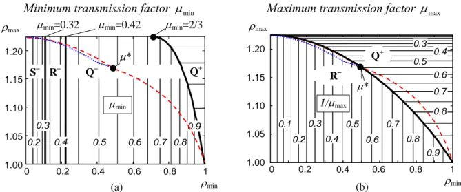
∈[0, 1] [1, 1.5]× .

Contour plots of global indices. Detailed investigation of the joint limit rectangle based on both

analytical and numerical tools has yielded results presented in Fig. 9, which contains the contour plots of μ_min,μ_max on the plane ρ_min,ρ_max. These plots are labelled by the relevant values of the velocity transmission factors and divided in separate areas, which differ by a type of the critical points. For instance, the contour plot for the function μ_min(ρ_min,ρ_max) consists of four areas,

, , Q S R− − −

and Q+, where the global transmission factors are defined by the critical points

{

S S S_x−, _y−, _z−

}

,

{

R R R_x−, _y−, _z−

}

, Q− and Q+ respectively. For comparison purposes, we also show by the dashed/dotted lines the one-dimensional subset of the joint limit rectangle, which corresponds to the “symmetrical” design constrains (i.e. μ_min =1 μ_max) imposed either on the full ρ-bounded workspace or along the Q-axis only.

As follows from Fig. 9a, the global minimum of the transmission factor can be achieved in either points S_i−, R_i−, or Q−, where i∈

{

x y z, ,

}

and all these indices are equivalent with respect to the

min, max

μ μ because of the symmetry. It has been proved, that particular expressions for computing of μ_min are

(

)

( )

]

]

( )

( )

( )

1 2 min SR 1 2 min SR RQ

min min max ₁

2 min RQ QQ max 1 + 1 min QQ max for 0, for , , Q for , ( ) Q for ( ), 1 i i S R λ ρ ρ λ ρ ρ ρ μ ρ ρ λ ρ ρ ϕ ρ λ ρ ϕ ρ − − − − − − − ⎧ _∈ ⎪ ⎪ _{⎤ ⎤} ∈ ⎦ ⎦ ⎪ = ⎨ ⎪ _{∈ ⎦}⎤ ⎤_⎦ ⎪ ⎪ _{∈ ⎦⎤ ⎡⎣} ⎩ (27)

where the subscripts of λ define the number of the critical singular value (1…3, in accordance with the above notation), and the critical points S_i−, R_i− and Q− are separated by the vertical lines

SR 0.1093

ρ = and ρ_RQ =0.2240 shown in bold in Fig. 9a (corresponding values of the transmission factor are μ_min

(

ρ_SR

)

=0.3232 and μ_min

( )

ρ_RQ =0.4210). The critical points Q+, Q− are separated by the curve ρ_min =ϕ_QQ

(

ρ_max

)

, which can be obtained by equating the eigenvalues λ₁ = +1 2χ and

2 1

λ = −χ for Q+ and Q− respectively. Hence, using the relation between the auxiliary variable χ and the joint coordinate along the Q-axis

(

)

2

1 1 2

ρ = −χ + χ , the equations for the function

(

)

QQ max

ϕ ρ can be presented both in the parametric

(

)

2

(

)

2

]

[

min 1 1 2 ; max 1 2 1 8 ; 0, 1 4

ρ = −χ + χ ρ = + χ + χ χ∈ (28a)

and explicit form

(

) (

(

)

)

2 2 2 2

max 3 3 2 min 9 2 min 4 min 3 2 min

ρ = − ρ − ρ − ρ − ρ ; ρ_min∈ ⎦⎤ 0.5, 1.0⎡_{⎣ . (28b)}

It can be also shown that along this curve the corresponding velocity transmission factor

(

)

min 1 1 2

μ = + χ varies from 1 to 2 3, and the curve is bounded by the points

( )

1, 1 and

(

0.5, 1.5 .

)

Minimum transmission factor μmin

0 0.2 0.4 0.6 0.8 1 1.00 1.05 1.10 1.15 1.20 μmin S− R− Q− Q+ 0.2 0.3 0.4 0.5 0.6 0.7 0.8 0.9 ρmin

ρmax μmin=0.32 μmin=0.42 μmin=2/3

(a) μ*

Maximum transmission factor μmax

0 0.2 0.4 0.6 0.8 1 1.00 1.05 1.10 1.15 1.20 0.1 R− 0.2 0.3 0.4 0.5 0.6 0.7 0.8 0.9 0.3 0.4 0.5 0.6 0.7 0.8 Q+ 1/μmax ρmin ρmax (b) μ*

Fig. 9. Contour plots of the global transmission factors μ_min,μ_max on the plane ρ_min×ρ_max (dashed/ dotted lines correspond to symmetrical constraints for Wρ/ Q-axis; μ∗ ≈0.54). Similar analysis for the global maximum of μmax (Fig. 9b) shows that it can be achieved in either

point R_i− or Q+, i.e.

(

)

( )

( )

1

1 max RQ min

max min max ₁ + 1 max RQ min for 1, ( ) , Q for ( ), 1.5 i R λ ρ ϕ ρ μ ρ ρ λ ρ ϕ ρ − − − ⎧ _{∈ ⎦⎤ ⎤} ⎦ ⎪ = ⎨ ⎤ ⎡ ∈ ⎪ _{⎦ ⎣} ⎩ (29)

where the subscripts of λ and R have similar meaning as in (27), and the critical points R_i−

and Q+ are separated by the curve ρ_min=ϕ_RQ

(

ρ_max

)

. This curve can be obtained by equating the eigenvalues λ₁= −1 χ and λ₁= +1 2χ respectively for R_i− and Q . Hence, using the relations + between the auxiliary variable χ and the joint coordinates of the Q-points ρ_Q = −

(

1 χ

)

1 2+ χ2 and R-point ρ_R = −

(

1 χ

)

1+χ2 , the equations for the function ϕ_RQ

(

ρ_max

)

can be presented both in the parametric

(

)

2

max 1 1 2 ;

ρ = −χ + χ ρ_min = +

(

1 2χ

)

1 4+ χ2; χ∈ −

]

1 2 , 0

[

. (30a) and explicit forms

(

)

(

)

2 max 2 min _{2 2}

max max max

9 3 2 15 2 4 3 2 ρ ρ ρ ρ ρ − = − − − ρmax∈ ⎦⎤1 , 3 2 ⎡⎣ . (30b)

It can be also shown that along this curve the corresponding velocity transmission factor

(

)

max 1 1 2

μ = + χ varies from 1 to ∞ , and the curve is bounded by the points

( )

1, 1 and

(

0, 1.5 .

)

Neighbourhood of the isotropic point. Since the kinematic design seeks for the quasi-isotropic

workspace, it is useful to obtain analytical expressions for μ_min in the neighbourhood of the isotropic point

( )

1, 1 , which is completely defined by the Q-axis (see Fig. 9a). As proved above, for both Q and Q+ − the auxiliary parameter χ may be expressed via the joint variable as

(

2

)

(

2

)

Q 1 3 2 2 1

χ = −ρ − ρ ρ − , hence in this case (27) may be reduced up to

min max QQ max 2 min min 2 max max 1 2 if ( ) 3 _{3 3 2} 3 2 2 otherwise 3 3 ρ _{ρ ϕ ρ} ρ μ ρ ρ ⎧ + ≥ ⎪ ₋ ⎪ = ⎨ − ⎪ + ⎪ ⎩ (31)

Rewriting these expressions with respect to μ_min yields

min min ₂ min min 3 1 Q : 6 4 2 μ ρ μ μ − _≥ − − + ; + max ₂ min min 1 Q : 3 4 2 ρ μ μ ≤ − + , (32)

which allow to compute the joint limits ρmin,ρmax for given design specification

0 min

μ ≥μ (provided that μmin ≥μ ρ

(

SR

)

≈0.32). For the wider range of μmin, the relevant equation was

0.0 0.5 1.0 1.5 μmin ≥ μ ρmax ρmin 0 0.2 0.4 0.6 0.8 1 μ Q+ Singularity Q− R− S− 0 0.2 0.4 μ 0.6 0.8 1 μmax≤ 1/μ ρmax ρmin Q+ R− 0.0 0.5 1.0 1.5

Fig. 10. Computing joint limits for non-symmetrical constraints (independent upper and lower bounding)

Similar expressions for μ_max can be derived by substitution of

(

2

)

(

2

)

min min min

1 2 1

R

χ = −ρ −ρ ρ − ;

(

2

)

(

2

)

Q 1 max 3 2 max 2 max 1

χ = −ρ − ρ ρ −

into equations for the roots λ₁= −1 χ_R and λ₁= +1 2χ_Q and relevant simplification:

max min RQ max 2 max max 2 min min 2 1 if ( ) 3 _{3 3 2} 2 1 otherwise 2 2 ρ _{ρ ϕ ρ} ρ μ ρ ρ ⎧ + ≤ ⎪ ₋ ⎪ = ⎨ − ⎪ ₊ ⎪ ⎩ (33)

Rewriting these expressions with respect to μ_max yields

min ₂ max max 1 R : 2 2 1 ρ μ μ − _≥ − + ; + max max ₂ max max 3 1 Q : 6 4 2 μ ρ μ μ − ≤ − + , (34)

which make it possible to compute the joint limits ρmin,ρmax for given design specification max 1

μ ≤ μ (see Fig. 10) .

Symmetrical design specification. The above results can be also used in the case of the

“symmetrical” design specification, which assumes the inverse relations between the upper and lower bound on the transmission factor (μ_min =1 μ_max), when the feasible workspace is defined by

the expression

( )

( )

{

min max

}

min , 1 Wρ μ μ μ ∈ ≥ p p p (35)

in which μ∈

[ ]

0, 1 is the value of the prescribed performance measure (for instance, it is natural to set the transmission factor to be in the range

[

1 2, 2

]

or

[

1 3, 3

]

, as it was proposed in [16]). As follows from the related analysis, in this case only two combinations of critical points are possible:

(

+

)

Q , Q− if μ μ≥ ∗ and

(

+

)

Q ,R_i− if μ μ< ∗, where μ∗ ≈0.5387, ρ_min

( )

μ∗ ≈0.4892,

( )

max 1.1700 ρ μ∗ _≈

(see Fig. 9). So, as follows from (31) and (33), the joint limits for the symmetrical design specification can be computed as

+ max ₂ 3 Q : , 0 1 2 4 6 μ ρ μ μ μ − ≤ < < − + (36a) min ₂ 3 1 Q : , 1 6 4 2 μ ρ μ μ μ μ − _≥ − ∗_{≤ <} − + ; R : min 2 , 0 2 2 μ ρ μ μ μ μ − _{≥ < <} ∗ − + (36b)

This relation is shown in Fig. 11a on the ρ_min×ρ_max plane and also plotted in Fig. 11b against the velocity transmission factor μ. They make it possible to evaluate the global manipulator performance for the whole ρ-bounded workspace W_ρ (for given joint limits) or to compute the joint limits that guarantee the desired performances throughout W_ρ.

0 0.2 0.4 0.6 0.8 1 1.00 1.05 1.10 1.15 1.20 ρmax ρmin 0.2 0.3 0.4 0.1 0.5 0.6 0.7 0.8 0.9 0.8 0.7 0.6 0.5 0.4 0.3 μ≤ μmin ; μmax ≤ 1/μ ( Q+,R− ) ( Q+_,Q− ₎ μ*=0.54 (a) 0.0 0.5 1.0 1.5 0 0.2 0.4 0.6 0.8 1 μ≤ μmin ; μmax ≤ 1/μ ρmax ρmin μ Q+, μmin μ* Q+ , μmax Q−, μmin R−, μmax R−, μmax Q+, μmax R−, μmin S−, μmin

Fig. 11. Transmission factors (a) and joint limits (b) for symmetrical constraints within W_ρ (dashed line shows symmetrical constraints for Q-axis only).

5.3. D

EFINING A CUBIC WORKSPACE

Since the prescribed Cartesian workspace has a cubic shape, let us first define the largest cube that ensures the desired transmission factors

[

μ μ through it, while temporarily releasing the joint , 1

]

limits constraints. It is obvious, that due to the Orthoglide symmetrical architecture, the cube faces must be parallel to the xy, xz and yz planes. So, the constraint (15) may be rewritten as

( )

( )

{

min max

}

min , 1 p W μ μ μ ∈ ≥ p p p (37)

where W denotes the p-bounded workspace determined by_p p p p_x, _y, _z∈

[

p_min, p_max

]

. Applying the above notation, the cube may be also defined by its two opposite vertices +

Q , Q− located on the bisector line. Detailed investigation of W using expressions from previous Sub-Sections is _p summarised in the following statement.

Proposition 1. If the prescribed symmetrical bounds μ

( )

p ∈

[

μ μ, 1

]

, 0< < on the velocity μ 1 transmission factors are satisfied at the Q-axis points +

Q , Q−, then these bounds are satisfied throughout the cubic workspace W defined by the vertices _p +

The proof of the proposition uses convexity of the workspace hull bounded by μ

( )

p ∈

[

μ μ, 1

]

and is based on comparing the Jacobian singular values in the critical points of the cubic workspace and on the expressions for the joint limits

( )

+

( )

2 2 2 3 3 1 Q ; Q max ; 2 4 6 6 4 2 2 4 3 μ μ μ ρ ρ μ μ μ μ μ μ − ⎧ ⎫ − ⎪ − ⎪ = = _{⎨ ⎬} − + _⎪⎩ − + − + _⎪⎭, (38)

which are derived from (31), (33). It should be noted that the ρ-bounded workspace defined by the same vertices Q , Q+ − does not satisfy the bounds

[

μ μ if , 1

]

μ μ< ∗≈0.54 (see Sub-Section 5.2), but the p-bounds remove the critical points R R_x+, _y+,...R_z−. Besides, utilising the cubic workspace with the vertices Q , Q+ − requires a certain enlargement of the upper joint limit. Really, as follows from the basic Orthoglide equations (1), the p-bounded Cartesian workspace maps into the joint space portion, which is contained in the parallelepiped

( ) ( )

+

, , Q , Q 1

x y z p

ρ ρ ρ _∈⎡ρ − _{+ ⎤}

⎣ ⎦ , (39)

where ρ

( )

Q− = p_min + 1 2− p_min2 is the joint coordinate at Q−, p

( )

Q+ = p_max is the Cartesian coordinate at +

Q , and p_min, p_max depend on the desired transmission factor bound μ and are computed from (31), (33). It can also be easily proved that

( )

+

( )

+

Q 1 Q

p + >ρ , since

( )

+ 2

max max

Q p 1 2p

ρ = + − (see Sub-Section 5.1). Hence, this increase in the upper joint limit may lead to the singularities included in the corresponding ρ-bounded workspace, which can be avoided only by adding some “software joint limits” (based on verifying of inequalities more complicated than ρmin ≤ρx≤ρmax and similar). Relevant computations showed that the singularity problem

arises for the transmission factors μ ≤ −1 1.5 1− ≈0.53 for which p

( )

Q+ + ≥1 1.5.

The alternative approach for defining the cubic workspace assumes that the joint limits corresponding to Q , Q+ − cannot be violated. Hence, the desired cube W_po should be completely

enclosed in the ρ-bounded space Wρ. It is obvious that Wpo ⊂Wp, so within the cube

o

p

W the manipulator possesses the desired kinematic properties. Dimension of the cube W_po and its spatial

location are defined by the following proposition.

Proposition 2. If the prescribed symmetrical bounds μ

( )

p ∈

[

μ μ, 1

]

, 0< < are satisfied in the μ 1 Q-axis points Q , Q+ −, then the largest cube enclosed in the ρ-bounded workspace W_ρ is defined by the vertices +

Q_∗ and Q−, where Q_∗+∈ ⎣⎡Q Q+ −⎤_{⎦ and} p

( ) ( )

Q_∗+ =ρ Q+ − . 1

The proof of this proposition is based on comparing the Cartesian coordinates for the critical points Q, R, S (see Fig. 8) and also uses the expression for the upper joint limit from Proposition 1. It is clear, that in this case the ρ-bounded workspace defined by Q , Q+ − is singularity-free, but its global performances may be out of the design specifications in R2-points and their neighbourhood if

0.54

μ < (see Sub-Section 5.2). So, the designer may choose the third design strategy, which guarantees satisfaction of the design specification both in the ρ-bounded and p-bounded workspaces W_ρ and W_po . The latter is based on the following corollary combining results from Propositions 1 and 2.

Corollary. If the prescribed symmetrical bounds μ

( )

p ∈

[

μ μ, 1

]

, 0< < are satisfied within the μ 1 ρ-bounded workspace defined by the vertices +

Q , Q− , then they are also satisfied within the p-bounded workspace defined by the vertices +

Q_∗ and Q−, withp

( ) ( )

Q+_∗ =ρ Q+ − . 1

These Propositions and Corollary give the designer three different methods (“design strategies”) for computing the joint limits and dextrous Cartesian workspace of the normalised manipulator (L=1), which afterwards must be scaled to achieve the prescribed workspace size. The methods are summarised in Table 3 and yield three Pareto-optimal solutions with respect to the design goals stated in Section 2. As follows from the propositions, all strategies ensure satisfaction of the design specification within the prescribed cubic workspace W , but differ by the manipulator _p performances in the remaining part W Wρ\ _p. It should be noted, that the primary version of the first method, for μ μ≥ ∗, was developed in the previous paper [16], while here it is generalised for the full range of the transmission factor.

Table 3

Computing joint limits for the unit Orthoglide

(dots on the Q-axis show location of Q , Q+ − for different design strategies).

Design strategies Remarks

Design strategy #1

(i) Compute points Q+, Q-to achieve required

transmission factors along segment Q+Q-.

(ii) Locate the cube vertices in points Q+, Q- to define

the cubic workspace W . _p

(iii) Adjust the joint limits to include the p-bounded workspace W inside the _p ρ-bounded one.

Q− Q+ - + min Q; max 1 pQ ; ρ =ρ ρ = + - + min Q; max Q ; p = p p = p

Inside the cube, design specifications are satisfied, but outside it, they are violated and even singularities exist

if μ ≤ 0.53

Design strategy #2

(i) Compute points Q+, Q- to achieve required

transmission factor along segment Q+Q- and set joint limits according to these points.

(ii) Inscribe the cube inside the ρ-bounded workspace W_ρ to define the cubic workspace W . _p

Q− Q+ - + min _Q; max _Q ; ρ =ρ ρ =ρ - + min Q; max Q 1; p = p p =ρ −

Workspace is singularity-free but, outside the cube, performances are

out of design specifications if 0.54μ<

Design strategy #3

(i) Compute points Q+, Q- to achieve required

transmission factor within the ρ-bounded workspace Wρ and set according joint limits.

(ii) Inscribe the cube inside the ρ-bounded workspace W_ρ to define the cubic workspace W . _p

Q− Q+ - + min _Q; max _Q ; ρ =ρ ρ =ρ - + min _Q; max _Q 1; p = p p =ρ −

Both ρ- and p-bounded workspaces are singularity-free and meet design

It is obvious that correctness of the above statements for the transmission factor guarantees their correctness for the manipulability and condition number indices, which may be directly expressed via the singular values. Also, for real-life problems, the designer can prefer one of the solutions to other ones taking into account a number of additional engineering constraints and objectives, which cannot be implicitly expressed in the frames of the model used in this paper.

6.

N

UMERICAL

E

XAMPLES AND

D

ISCUSSIONS

To compare the proposed design approaches, let us apply them to the design of the Orthoglide for the unit Cartesian workspace c c c× × , c=1 with the transmission factors bounds 0.5≤ ≤μ 2.0 . As stated above, the design process includes two main stages: (i) defining the joint limits ρ_min,ρ_max for the normalised manipulator with the link length L= , and (ii) scaling the manipulator 1 parameters

(

ρ_min,ρ_max,p_min,p_max,L

)

to achieve the prescribed workspace size.

For the normalised manipulator, the Q-axis technique gives the following ranges for the joint/Cartesian coordinates and corresponding transmission factors within the ρ- and p-bounded workspaces μ

( )

W_ρ , μ

( )

W_p , which are called below J-Space and C-Space, respectively (i.e. “Joint-coordinate bounded space” and “Cartesian-coordinate bounded space”):

J-Space0: ρ∈

[

0.4082, 1.1785 ;

]

Δ =ρ 0.7703; μ

( )

Wρ ∈

[

0.50, 2.16

]

C-Space0: p∈ −

[

0.4082, 0.2357 ;

]

Δ =p 0.6440; μ

( )

Wp ∈

[

0.50, 2.00

]

Strategy #1 assumes that the cube with the edge pΔ is used as the prescribed Cartesian workspace. It requires increasing the upper joint limit to make all points of the cube attainable. According to Sub-Section 5.3, the enlarged joint space is defined as

J-Space1: ρ∈

[

0.4082, 1.2357 ;

]

Δ =ρ 0.8275; μ

( )

Wρ =

[

0.50, ∞

[

So, since ρ_max> 1.5, the obtained ρ-bounded workspace includes parallel singularities, which may be eliminated by additional software constrains on the joint coordinates. For instance, the inequality

Q

3

x y z

ρ +ρ +ρ ≤ ρ + removes the singularities from W_ρ and restores the original transmission

factors

[

0.50, 2.16

]

.

Strategy #2 keeps the original ρ-bounded workspace, within which is located the prescribed cube. Computing relevant parameters gives:

C-Space2: p∈ −

[

0.4082, 0.1785 ;

]

Δ =p 0.5868; μ

( )

W_p =

[

0.50, 2.00

]

In this case, the cube is smaller but the workspace is singularity-free and possesses reasonable kinematic properties both inside and outside the cube.

Strategy #3 provides the desired transmission factors for the whole ρ-bounded workspace, which is computed in accordance with Table 3 and is defined as

J-Space3: ρ∈

[

0.4472, 1.1785 ;

]

Δ =ρ 0.7313; μ

( )

Wρ =

[

0.52, 2.00

]

Then, inscribing the largest cube gives

C-Space3: p∈

[

-0.3884, 0.1785 ;

]

Δ =p 0.5669; μ

( )

Wp =

[

0.52, 1.87

]

that overtakes the required kinematic performances for the cube but ensures them for the whole ρ -bounded workspace.

After defining normalised manipulator parameters, the obtained cubic workspaces must be adjusted to the prescribed size c c c× × by scaling the manipulator dimensions and joint/Cartesian coordinates. Computing the scaling factor η=c Δρ for c=1 yields 1.553, 1.704 and 1.764 for the first, second and third design strategies respectively. Design results after scaling are summarised in Table 4, which also contains ratio of the actuated joints range Δ to the cube size c. These results ρ shows that all obtained solutions are Pareto-optimal with respect to the vector criterion

(

L,μmin,μmax

)

with the goals L→min and μmin,μmax →1.0 . Indeed, Strategy #1 yields the

smallest Orthoglide dimensions (about 12% less than the third one), but the worst kinematic properties outside the cube (with singularities). In contrast, Strategy #3 guarantees the best kinematic performances for the price of the largest manipulator links, while Strategy #2 gives an intermediate solution ensuring the compromise between the link length and transmission factors. Hence, none of the strategies can be given a preference within the frames of the kinematic model and, in real-life applications, all these solutions should be presented to the designer who may evaluate them by taking into account a number of additional technical constraints and goals.

Table 4

Orthoglide parameters and performances for W_p = × × and 0.51 1 1 ≤ ≤μ 2.0 Design strategy L ρ min ρmax Δ ρ c Δρ μ

( )

Wp μ

( )

Wρ #1 1.553 0.634 1.919 1.285 0.7782 0.500 … 2.000 singularity #2 1.704 0.696 2.009 1.313 0.7618 0.500 … 2.000 0.500 … 2.158 #3 1.764 0.789 2.079 1.290 0.7752 0.518 … 1.869 0.518 … 2.000

Finally, let us demonstrate application of the proposed technique to the design of the Orthoglide prototype, which has been built in Institut de Recherche en Communications et Cybernétique de Nantes (IRCCyN). The prescribed performances of the manipulator are: Cartesian velocity and acceleration in the isotropic point 1.2 m/s and 14 m/s2 ; payload 4 kg ; cubic Cartesian workspace size 200 200 200× × mm ; transmission factor range 0.5 ÷ 2.0 . Application of the design strategies #1,…3 yielded the Orthoglide link lengths 310.6, 340.9, 352.8 mm respectively. Taking into account additional technical goals related to the manipulator mass and dynamic performances, the preference was given to the solution with the smallest link length. Corresponding joint limits are

min 126.8 mm

ρ = and ρ_max =383.8 mm. To remove singularities, the software constraint

Q

3

x y z

ρ ρ ρ+ + ≤ ρ + were used where

Q

3ρ + =1098.1 mm. As follows from simulation and laboratory experiments, the prototype ensures required transmission factors within the prescribed cubic workspace [0.50, 2.00] and also their reasonable values outside the cube [0.50, 2.16]. However, during tuning of the control system, it was noticed rather high sensitivity of the kinematic performances with respect to the joint encoder offset. For instance, the 5 mm offset leads to changing of the Cartesian cube transmission factors to [0.50, 2.42]. The 10 mm offset increases their range up to [0.50, 3.42]. This imposes strict requirements on the assembly accuracy and motivates dedicated research on the Orthoglide calibration.

7.

CONCLUSIONS

The paper focuse on the parametrical synthesis of the Orthoglide, a parallel manipulator for 3-axis rapid machining applications, which combines advantages of both serial mechanisms (regular workspace and homogeneous performances) and parallel kinematic architectures (good dynamic performances). Three strategies have been proposed to define the Orthoglide geometric parameters as functions of a cubic workspace size and dextrous properties expressed by bounds on the velocity transmission factors, manipulability or the Jacobian condition number. Low inertia and intrinsic stiffness have been set as additional design goals expressed by the minimal link length requirement. In contrast to previous works, we proposed several Pareto-optimal solutions of the design problem, which differ by the manipulator performances outside the prescribed Cartesian cube (but within the workspace bounded by the actuated joint limits). Taking into account linear relation between the manipulator parameters and the cubic workspace size, the design process is decomposed in two stages: (i) defining the actuated joint limits and the largest cube size/location to satisfy the dexterity goals for the normalised manipulator; (ii) scaling the normalised manipulator to satisfy a specification on the cubic workspace size.

For each design strategy, we proposed analytical expressions for computing the Orthoglide parameters, which were based on the “critical points” concept that allows evaluating the global performance indices through the joint-bounded or cubic workspaces without their exhaustive exploration. We also proved two propositions describing relations between these workspace sizes and kinematic performances within them. It was shown, that independently of the applied strategy, the workspace includes the fully-isotropic point where any linear joint displacement yields similar manipulator tool displacement, like in a serial XYZ-machine. So, the synthesis is aimed at specifying the cubic volume around this point, which meets the dexterity goals. The related design parameters are the actuated joint limits and manipulator link lengths.

The proposed design strategies have been illustrated by numerical examples with the dexterity specification expressed by the velocity transmission factor. We obtained three Pareto-optimal solutions ensuring the required kinematic properties within the cubic workspace but providing wider range of the transmission factor outside the cube (this range is decreased monotonously while the manipulator link length is increased). Hence, no one of the strategies can be given a preference within the frames of the kinematic model and, in real-life applications, all the solutions should be presented to the designer who should evaluate them taking into account additional technical constraints and goals.

The developed technique has been also applied to the design of the Orthoglide prototype, which has been successfully built and tested in IRCCyN (Nantes, France). However, experiments with this manipulator showed rather high sensitivity of the kinematic performances with respect to the joint encoder offsets, which motivates further research on the Orthoglide calibration.

REFERENCES

[1] J.-P. Merlet, Parallel Robots, Kluwer Academic Publishers, Dordrecht, 2000.

[2] J. Tlusty, J.C. Ziegert, S. Ridgeway, Fundamental Comparison of the Use of Serial and Parallel Kinematics for Machine Tools, CIRP Annals 48 (1) (1999) 351-356.

[3] P. Wenger, C. Gosselin, B. Maille, A comparative study of serial and parallel mechanism topologies for machine tools, in: Proceedings of PKM’99, Milan, Italy, 1999, pp. 23–32. [4] L.W. Tsai, Robot Analysis: the Mechanics of Serial and Parallel Manipulators; John Wiley &

Sons, New York, 1999.