HAL Id: hal-02938091
https://hal.archives-ouvertes.fr/hal-02938091
Submitted on 5 Jan 2021HAL is a multi-disciplinary open access archive for the deposit and dissemination of sci-entific research documents, whether they are pub-lished or not. The documents may come from teaching and research institutions in France or abroad, or from public or private research centers.
L’archive ouverte pluridisciplinaire HAL, est destinée au dépôt et à la diffusion de documents scientifiques de niveau recherche, publiés ou non, émanant des établissements d’enseignement et de recherche français ou étrangers, des laboratoires publics ou privés.
Linking Spatial and Temporal Dynamic of
Bacterioplankton Communities With Ecological
Strategies Across a Coastal Frontal Area
Clarisse Lemonnier, Morgan Perennou, Damien Eveillard, Antonio
Fernandez-Guerra, Aude Leynaert, Louis Marié, Hilary Morrison, Laurent
Mémery, Christine Paillard, Lois Maignien
To cite this version:
Clarisse Lemonnier, Morgan Perennou, Damien Eveillard, Antonio Fernandez-Guerra, Aude Leynaert, et al.. Linking Spatial and Temporal Dynamic of Bacterioplankton Communities With Ecological Strategies Across a Coastal Frontal Area. Frontiers in Marine Science, Frontiers Media, 2020, 7, �10.3389/fmars.2020.00376�. �hal-02938091�
Linking Spatial and temporal dynamic of bacterioplankton
communities with ecological strategies across a coastal frontal area
1C. Lemonnier1,2, M. Perennou2, D. Eveillard3, A. Fernandez-Guerra4,5,6, A. Leynaert2, L.
2
Marié7, H.G. Morrison8, L. Memery2, C. Paillard2 and L. Maignien1,8
3 4
1Univ Brest (UBO), CNRS, IFREMER, Laboratoire de Microbiologie des Environnements Extrêmes,
5
F-29280 Plouzané, France 6
2Univ Brest (UBO), CNRS, IRD, Ifremer, Laboratoire des Sciences de l’Environnement Marin,
F-7
29280 Plouzane, France 8
3Univ Nantes, CNRS, Centrale Nantes, IMTA, Laboratoire des Sciences Numériques de Nantes,
F-9
44322 Nantes, France 10
11
4Microbial Genomics and Bioinformatics Research Group, Max Planck Institute for Marine
12
Microbiology, Bremen, Germany 13
14
5 Lundbeck Foundation GeoGenetics Centre, GLOBE Institute, University of Copenhagen, Øster
15
Voldgade 5-7, 1350 Copenhagen K, Denmark 16
17
6University of Bremen, Center for Marine Environmental Sciences, 28359 Bremen, Germany
18 19
7Univ. Brest, CNRS, IRD, Ifremer, Laboratoire d'Océanographie Physique et Spatiale, F-29280
20
Plouzané, France 21
8Marine Biological Laboratory, Josephine Bay Paul Center for Comparative Molecular Biology and
22
Evolution, Woods Hole, MA, United States 23 24 * Correspondence: 25 Loïs Maignien 26 lois.maignien@univ-brest.fr 27 28 29
Keywords: Marine front, bacterial communities, dynamic, network, ecological strategies
30 31
32
Abstract
33
Ocean frontal systems are widespread hydrological features defining the transition zone between 34
distinct water masses. They are generally of high biological importance as they are often associated 35
with locally enhanced primary production by phytoplankton. However, the composition of bacterial 36
communities in the frontal zone remains poorly understood. In this study, we investigate how a coastal 37
tidal front in Brittany (France) structures the free-living bacterioplankton communities in a spatio-38
temporal survey across four cruises, five stations and three depths. We used 16S rRNA gene surveys 39
to compare bacterial community structures across 134 seawater samples and defined groups of co-40
varying taxa (modules) exhibiting coherent ecological patterns across space and time. We found that 41
bacterial communities composition was strongly associated with the biogeochemical characteristics of 42
the different water masses and that the front act as an ecological boundary for free-living bacteria. 43
Seasonal variations in primary producers and their distribution in the water column appeared as the 44
most salient parameters controlling heterotrophic bacteria which dominated the free-living community. 45
Different dynamics of modules observed in this environment were strongly consistent with a 46
partitioning of heterotrophic bacterioplankton in oligotroph and copiotroph ecological strategies. 47
Oligotroph taxa, dominated by SAR11 Clade members, were relatively more abundant in low 48
phytoplankton, high inorganic nutrients water masses, while copiotrophs and particularly opportunist 49
taxa such as Tenacibaculum sp or Pseudoalteromonas sp reached their highest abundances during the 50
more productive period. Overall, this study shows a remarkable coupling between bacterioplankton 51
communities dynamics, trophic strategies, and seasonal cycles in a complex coastal environment. 52
1 Introduction
54
Bacteria dominate the marine environment in abundance, diversity and activity where they 55
support critical roles in the functioning of marine ecosystems and oceanic biogeochemical cycles 56
(Falkowski et al., Fenchel, and Delong 2008; Cotner and Biddanda 2002; Madsen 2011). In the coastal 57
environment, they are closely associated with other planktonic organisms (e.g. viruses, phytoplankton 58
and zooplankton) during the recycling of organic matter and inorganic nutrients through the so-called 59
microbial loop (Azam and Malfatti 2007; Pomeroy et al. 2007). They form complex and highly 60
dynamic assemblage (S. J. Giovannoni and Vergin 2012), with bacterioplankton diversity variations in 61
space and time linked to changes in functional diversity (Galand et al. 2018). Therefore, understanding 62
how the bacterioplankton composition varies in the environment remains one of the central question 63
to elucidate so that we can better understand coastal ecosystem functioning (Fuhrman et al. 2015). 64
Phytoplankton development represents a major source of organic matter for heterotrophic 65
bacteria in the water column. During their growth and upon bloom termination, algae release a complex 66
bulk of dissolved organic matter that is almost only available for bacteria (Azam 1998; Fenchel and 67
Jørgensen 1977). This organic matter processing requires diverse heterotrophic bacterioplankton 68
among which one could find members of Bacteriodetes (Flavobacteriacae), Roseobacter group, 69
Gammaproteobacteria and Verrucomicrobia (Buchan et al. 2014). These taxa contribute to the
70
complexity of the marine ecosystem via different adaptive strategies, owing to the unequal access to 71
their respective resource (Stocker 2012; Luo and Moran 2014). For instance, heterotrophs are generally 72
distinguished as either oligotrophs or copiotrophs that compete at low and high nutrient concentrations 73
respectively (Koch 2001; Giovannoni et al. 2014). They also present different degrees of ecological 74
specialization, with generalist bacteria able to assimilate a broad variety of substrates, while specialists 75
will compete for a narrow range of nutrients (Mou et al. 2008). Analysis of these ecological traits offer 76
a simplified view of complex microbial communities and has gained interest for better understanding 77
the dynamics of natural microbial communities and to gain insight into their role in the ecosystem 78
(Krause et al. 2014; J. Raes et al. 2011; Haggerty and Dinsdale 2017). 79
Marine fronts are common mesoscale features in the ocean and are located at the transition 80
between water masses of different physicochemical characteristics that actively shape the distribution 81
of microbial organisms (phytoplankton, zooplankton and bacteria). Driven by currents and mixing, 82
local nutrient input in the vicinity of the front generally enhances primary and secondary production, 83
making the frontal zone an area of high biological importance (Olson and Backus 1985) and of critical 84
influence on the microbial processing of organic matter (Baltar et al. 2015; Heinänen et al. 1995). 85
However, the bacterial communities' composition involved in such dynamic systems remains to be 86
investigated (Baltar et al. 2016). 87
The Ushant Front in the Iroise Sea (Brittany, France) is considered as a model for coastal tidal 88
front (Le Fèvre 1986). Its position and characteristics are highly dynamic and influenced by 89
atmospheric forcing and tidal currents which are strong in this area (Le et al. 2009). It occurs from May 90
to October and leads to contrasting physicochemical environments with higher phytoplankton biomass 91
at the frontal area (Le Fèvre et al. 1983). West of the front, stratification results in warmer oligotrophic 92
surface waters and colder nutrient-rich deeper waters separated by a marked thermocline. East of the 93
front, associated with highly variable conditions, permanently mixed coastal waters are characterized 94
by an unlimited quantity of inorganic nutrients but with highly fluctuating conditions. These 95
contrasting water masses structure the distribution of primary producers with the dominance of small 96
phytoplankton and dinoflagellates in surface stratified waters and diatoms in mixed waters (Birrien et 97
al. 1991; GREPMA 1988; Videau 1987). 98
In this study, we investigated how such contrasting physicochemical and biological parameters will 99
drive free-living bacterioplankon community structure. We then tested the hypothesis that the 100
contrasted distribution of primary producers will select for bacteria with different adaptative strategies. 101
To do so, using a network analysis we defined groups of co-varying bacterial OTUs that present the 102
same dynamic across the samples, postulating that they may share the same ecological niches. 103
104
Materials and Methods
105 106
1. Study site and sampling design 107
108
For this study, we completed four east-west transects of about 60 km across the Iroise sea in September 109
2014 (the 9th, 10th and 11th), March 2015 (the 10th, 11th and 12th), July 2015 (the 1st, 2nd and 3rd) 110
and September 2015 (the 8th, 9th and 10th) aboard the R/V Albert Lucas. Station positions remained 111
identical across cruises and were designed to span the front (Fig. 1A). Station 5 (48°25 N, 5°30 W) is 112
the most offshore station and is characterized by a strong stratification in summer. Station 4 (48°25 N, 113
5°20 W) and Station 3 (48°20 N, 5°10 W) are closer the front. Station 2 (48°15 N, 5°00 W) is present
114
in the mixed area and Station 1 (48°16 N, 4°45 W) is the most coastal station, near the outflow of the 115
Bay of Brest. At each station, we obtained CTD profiles to assess the physical characteristics of the 116
water column and establish the depth designed to capture the important biological and chemical 117
features of the water column at the surface, bottom and Deep Chlorophyll Maximum (DCM). 118
119 120
2. Nutrients, phytoplankton counts and pigment analyses 121
122
Seawater was sampled at each depth for nutrients, biogenic silica (BSi), chlorophyll a (Chl a), 123
particulate organic carbon and nitrogen (POC/PON) concentrations, and microscopic phytoplankton 124
cell counts and identification. Dissolved inorganic phosphate (DIP) and silicate (DSi) concentrations 125
were determined from seawater filtered on Nucleopore membrane filters (47 mm) and dissolved 126
inorganic nitrogen (DIN) on Whatman GF/F filters (25 mm). Filters for DIN and DIP were then frozen, 127
whereas filters for DSi were kept at 4 °C in the dark. Concentrations were later determined in the 128
laboratory by colorimetric methods using segmented flow analysis (Auto-analyser AA3HR Seal-129
Analytical) (Aminot and Kérouel 2007). BSi was determined from particulate matter collected by 130
filtration of 1 L of seawater through 0.6 μm polycarbonate membrane filter. The analysis was 131
performed using the alkaline digestion method (Ragueneau and Tréguer 1994). Total Chl a and 132
phaeopigments (Pheo) were determined in particulate organic matter collected on 25 mm Whatman 133
GF/F filters. The filters were frozen (-20°C) and analyzed later by a fluorometric acidification 134
procedure in 90% acetone extracts (Holm-Hansen et al. 1965). Particulate material for POC/PON 135
measurements was recovered on pre-combusted (450 °C, 4 h) Whatman GF/F filters. Samples were 136
then analyzed by combustion method (Strickland and Parsons 1972), using a CHN elemental analyzer 137
(Thermo Fischer Flash EA 1112). Phytoplankton samples were fixed with Lugol’s solution and cell 138
counts were carried out using the Lund et al. (1958) method (Lund et al. 1958). 139
140 141
3. Bacterioplankton community sampling 142
143
Seawater for bacterial diversity analysis was collected at different depths using Niskin bottles and 144
directly poured in 5 L sterile carboys previously rinsed three times with the sample. For each depth, 145
three biological replicates samplings were done, consisting of three different Niskin deployments, 146
except Station 4 in September 2014. Filtrations started in the on-shore laboratory 3 to 4 hours after 147
sampling. Water samples were size-fractionated using three in-line filters of different porosity: 10 µm, 148
3 µm (PC membrane filters, Millipore®) and 0.22 µm (Sterivex® filters, with PES membrane). In this 149
study, we focused only on the 0.22-3 µm free-living fraction. All filters were frozen in liquid nitrogen 150
before storage at -80 °C. In total, 2 to 5 liters of seawater were filtered each time, depending on filter 151
saturation. 152
153 154
4. DNA extraction and sequencing 155
156
Half-filters were directly placed in Matrix B® tubes (filled with 0.1 mm silicate beads, MP 157
Biomedicals) with lysis buffer (Tris pH 7.0, EDTA pH 8.0 and NaCl), SDS 10% and Sarkosyl 10% 158
and subjected to physical lysis for 5 minutes on a vortex plate. The liquid fraction was then collected 159
in order to perform a phenol-chloroform extraction using PCI (Phenol, Cholorophorm Isoamyl alcohol 160
with a ratio of 25:24:1) and a precipitation step with isopropanol and 5 M sodium acetate. DNA was 161
resuspended in 100 µL of sterile water. 162
Bacterial diversity was assessed by targeting the v4-v5 hypervariable regions of 16S rDNA with the 163
primers 518F (CCAGCAGCYGCGGTAAN) / 926R (CCGTCAATTCNTTTRAGT– 164
CCGTCAATTTCTTTGAGT - CCGTCTATTCCTTTGANT) (Nelson et al. 2014). PCR products 165
were purified using Ampure XP® kit and DNA quantity was measured using Picogreen® staining and 166
a plate fluorescence reader (TECAN® infinite M200 Pro). Each sample was diluted to the same 167
concentration and pooled before sequencing on an Illumina MiSeq sequencer at the Marine Biological 168
Laboratory (Woods Hole MA, USA). 169 170 171 5. Bioinformatics analysis 172 173
We obtained 22,523,398 raw reads, with a range from 31,583 to 2,001,687 reads per sample. Reads 174
were merged and quality-filtered according to recommendations in Minoche et al. (Minoche et al., 175
2011) using the Illumina-utils scripts (Eren et al. 2013). Those steps removed 17 % of all the sequences. 176
We used the Swarm algorithm (Mahé et al. 2014) to cluster the 18,876,655 remaining sequences into 177
1,611,447 operational taxonomic unit OTUs. Chimera detection was done using vsearch de novo 178
(Rognes et al. 2016) resulting in 281,825 filtered OTUs. Taxonomic annotation for each OTU was 179
done with the SILVA database v123 (Quast et al. 2012) using the mothur classify.seqs command 180
(Schloss et al. 2009). 19,516 OTUs (1,247,339 sequences) were affiliated with non-bacterial taxa (e.g. 181
archaea, chloroplasts, mitochondria, eukaryota) and removed from the dataset. As a result, we obtained 182
262,308 OTUs for 134 samples, with a large number of singletons (205,292 OTUs), that were kept 183
along the statistical analysis. 184 185 186 6. Statistical analysis 187 188
Libraries were normalized for read number using DESeq package in R (Anders and Huber 2010). A 189
visualization of the bacterial community structure similarity was assessed with an NMDS based on 190
Bray-Curtis dissimilarities using vegan R package (Oksanen et al. 2007). Influence of depth, station 191
and sampling time on bacterial communities was investigated using a permutational multivariate 192
analysis of variance (PERMANOVA) based on Bray-Curtis dissimilarities and 999 permutations. We 193
used principal coordinate analysis (PCA) ordination to characterize water samples environmental 194
parameters. Finally, we examined the presence of biomarker OTUs (i.e. OTUs with a significant higher 195
relative abundance in a given condition) of the different stations within each cruise using the LEfSe 196
software (Segata et al. 2011). 197
198
7. Network analysis 199
200
Network analysis was done based on a truncated matrix only containing the most abundant OTUs with 201
more than 50 sequences in at least three samples. The filtered matrix contained 681 OTUs that 202
accounted for 79% of all the sequences. This filtering step was necessary to avoid false positive 203
correlations in the network analysis. Our module detection analysis followed part of the pipeline of 204
Chafee et al. (Chafee et al. 2018). First, the application of SPIEC-EASI computes pairwise co-variance 205
based correlation between OTUs in order to address the sparsity and composition issues inherent to 206
microbial abundance data (Kurtz et al. 2015). The possible interaction was then inferred using the 207
glasso probabilistic inference model with a lambda.min.ratio of 0.01. Based on this model, only the 208
significant covariance values were extracted and transformed into a correlation matrix using the 209
cov2cor() function. 210
We then delineated network modules as groups of highly interconnected OTUs that presented very 211
close variations in relative abundances across the studied samples. Those modules were defined using 212
the Louvain algorithm (Blondel et al. 2008). We used Gephi (Bastian et al. 2009) and Force Atlas 2 213
layout algorithm to generate a vizualization of the main correlations (>0.3). Module eigengenes (ME, 214
the first principal component, considered a representative of the OTUs distribution of a given module) 215
were calculated based on the relative abundance matrix using WGCNA function moduleEigengenes() 216
(Langfelder and Horvath 2008). Those ME were used to calculate Pearson correlations between the 217
different modules and the environmental variables, using the WGCNA commands moduleTraitCor(), 218
moduleTraitPvalue(). 219
We used the methods proposed by Newton et al. to infer the trophic strategy of OTUs within each 220
modules (Newton and Shade 2016). In that study, they differentiated opportunist taxa with high 221
abundance variability in space and time, and marathoners with low abundance variability. They 222
distinguished these using the Coefficient of Variation (CV) of OTU dynamic combined with their 223
abundance and prevalence in the samples. Based on their method, we defined high CV opportunist 224
OTUs (or HCV) as OTUs above 5% upper boundary of the linear modeling 95% confidence interval 225
in a CV plot against OTU occurrence. Conversely, we defined low CV marathoners OTUs (or LCV) 226
as OTUs below the 5% lower boundary of the linear modeling. In our analysis, OTU occurrence was 227
defined by a relative abundance > 0.05%. 228
229
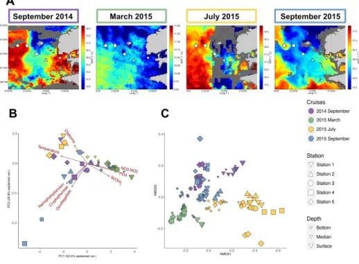
All the scripts used for this analysis are available at: https://loimai.github.io/BBobs/ 230 231 Results 232 1. Environmental settings 233
This study was carried out between September 2014 and September 2015 in the Iroise Sea, off 234
Brittany (Northeast Atlantic), in the vicinity of the Ushant island. The Ushant front position and 235
characteristics were estimated using Satellite Surface Temperature (SST) maps (Fig. 1) and CTD data 236
collected at the dates of sampling (suppl. data 1). The March 2015 sampling took place before the onset 237
of the Ushant front and presented a homogeneous temperature around 10 °C across all the stations. 238
High nutrient concentrations at all stations (Si(OH)4: 1.82 to 4.38 µM, nitrates: 5.88 to 12.13 µM,
239
suppl. data 2), low surface Chl a (<1 µg.L-1 except for Station 1, suppl. data 3) and overall low 240
phytoplankton cells counts observed during this cruise (suppl. data 2) indicated that sampling occurred 241
prior to the development of the phytoplankton spring blooms. In summer (September 2014, July 2015 242
and September 2015), SST maps showed a sharp transition between coastal and offshore temperatures 243
confirming the presence of a frontal system. The different observed stratification regimes (suppl. data 244
1) coincided with distinct physicochemical patterns and phytoplanktonic patterns across seasons (Fig. 245
1B, suppl. data 2). In late summer (September samples), offshore deep waters shared close 246
characteristics with winter waters (March sample, Temperature: 11.7 to 12.3 °C), with few 247
phytoplankton cells, similar concentration of Si(OH)4 (1.61 to 3 µM) and nitrates (3.99 to 6.41 µM).
248
Conversely, surface waters presented high temperatures (14.7 to 18.2 °C), a nutrient depletion 249
(Si(OH)4: 0.02 to 1.65 µM, N02+N03: 0.00 to 0.09 µM) and high phytoplankton cell counts. In early
250
summer (July), inorganic nutrient concentrations were overall lower than in September, probably 251
consumed by the spring bloom coinciding with the onset of the front around May-June. A significant 252
bloom occurred at stations 2 and 3, on the 27th of June, five days before the sampling period as seen 253
in the satellite surface Chl a observations (suppl. Data 3 B.). 254
2. Bacterial community dynamics in the Iroise Sea 256
In the Iroise Sea, free-living bacterial communities structure presented clear time and spatial 257
patterns as shown in the NMDS ordination plot (Fig. 1C, for each cruise separately see suppl. Data 4). 258
Firstly, community structure displayed strong seasonality, with sample primarily grouping by sampling 259
cruises. We also observed similar communities in stratified waters of September 2014 and 2015 260
samples (Fig. 1C), suggesting that these seasonal pattern were recurring . 261
Besides, we also observed an important spatial influence, as within each sampling cruise, 262
communities were markedly different between stations. In winter samples, communities were highly 263
similar throughout the water column (Depth was non-significant, Permanova Pr(>f) =0.225), but 264
presented a coastal to offshore gradient (Station was significant, Permanova Pr(>f) =0.001, suppl. Data 265
4) that followed a gradient of salinity, temperature and inorganic nutrient (sup. data 2). Conversely, in 266
September, when the front was the strongest, free-living bacterial communities were much more 267
heterogeneous with clear patterns associated to the set-up of the front : stratification resulted in highly 268
diverging communities with depth (Depth Pr(>f) = 0.004), while this pattern was not seen for the mixed 269
and coastal samples (Depth was not significant, Pr(>f) = 0.222 and 0.434, suppl. Data 4). In July, the 270
patterns were mostly associated with depth for all the stations, except station 1 (suppl. Data 4). 271
Overall, bacterial communities structure followed the different water masses, mirroring environmental 272
physicochemical variations represented in the PCA plot of environmental variables (Fig. 1B): deep 273
water communities in the summer crews remained more similar to winter communities (Fig. 1C). In 274
contrast, surface bacterial communities in stratified regimes and in most of the stations in July departed 275
from this typical winter structure. In addition, for these summer cruises, the DCM samples either cluster 276
with surface or deep samples. This could be explained by the difficulty to sample the DCM precisely, 277
as its depth can vary between the CTD measurements and the biological sampling. 278
Using the LefSe algorithm (Segata et al. 2011), we found that some stations displayed specific 279
biomarker OTUs within each sampling time (suppl. Data 5). Biomarkers such as OTU1 (Amylibacter) 280
and OTU4 (Planktomarina) were found at the most near-shore station (Station 1) in September 2014 281
and March 2015 and other biomarkers were found in surface stratified waters in early summer (OTU29 282
NS4 marine group) and late summer (OTU10 Synechococcus) cruises, but no biomarker was identified
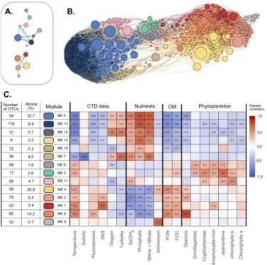
283
for the mixed and frontal stations except in July 2015 at Station 2 with OTU35 (Aliivibrio) and OTU74 284 (Pseudoalteromonas). 285 286 8. Description of modules 287
We further investigated groups of co-varying OTUs that could potentially share the same 288
ecological niches in this partitioned marine environment via a co-occurrence network analysis. In the 289
inferred network, we were able to identify 14 sub-networks (Fig. 2A and 2B) defining groups of OTUs 290
(termed modules) with similar distribution patterns across the entire study. Two modules (5 and 4) 291
were dominant in our dataset and respectively accounted for 32.7% and 20.9% of all sequences. Eight 292
modules represented between 1.6% and 14.2%, and four were rarer with less than 1% abundance. The 293
OTU taxonomy in each module is summarized in suppl. Data 6 and Fig. 4 presents the distribution of 294
the dominant families among each module. 295
Since its eigengene could characterize each module, we investigated to which extent module 296
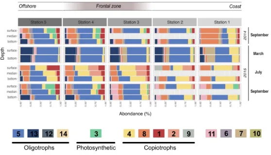
distribution could be correlated (i.e. Pearson correlation) with environmental parameters (Fig. 2C). 297
Correlation patterns partitioned modules into three significant sub-networks. The first one mostly 298
comprises modules 5 and 13 representing 32.7 and 6.8% of the dataset respectively that correlated 299
positively to inorganic nutrient concentrations and negatively to temperature and Particulate Organic 300
Matter (POC, PON) values. Their relative abundance in the different samples showed that they were 301
dominant in oligotrophic waters: together they ranged from 39% at Station 1 to 72% at Station 5 of the 302
late winter communities, and 54% to 59% of the deep stratified waters in September (Fig. 3). SAR11 303
Surface 1 (46.7% of the module sequences), ZD0405 marine group (12%) and SAR86 Clade (6.4%) 304
dominate the main module (module 5). Module 13 showed a different diversity as being dominated by 305
members of Marinimicrobia (15.8%), SAR11 Deep 1 (12%), SAR11 Surface 1 (8.9%) and 306
Salinisphaeraceae (7.9%).
307
Modules 4, 8, 2 and 1 contributed to the second sub-network, representing 20.9, 14.2, 5.5 and 308
5.4% of the dataset respectively. They presented clear inverse correlations compared with modules of 309
the first group: they correlated positively with temperature, POM and Diatoms but negatively with 310
inorganic nutrient concentrations. In relative abundance, they dominated the samples of July and in the 311
surface and coastal stations. Their taxonomy was distinct from the first group; i.e. together they 312
gathered the majority of Flavobacteriaceae (70%) and Rhodobacteraceae (88%). Also, module 9 was 313
enhanced in July 2015 but was almost exclusively present in Station 2 and strongly correlated with 314
ammonium (0.72, p < 0001). Its taxonomy was also particular as dominated by Vibrionaceae (58%) 315
and Pseudoalteromonadaceae (30%). 316
The third sub-network (modules 6 and 3) was less abundant and presented different correlations 317
with environmental parameters. They respectively account for 1.6 and 2.6% of the dataset, were 318
correlated with specific phytoplankton groups (dinoflagellates, nanophytoplankton) and were 319
dominant in the surface and DCM of stratified waters in September where they made up to 34% of the 320
community. Among them, module 3 was constituted almost exclusively of Cyanobacteria (94%) 321
affiliated with the Synechococcus genus. 322
To examine whether the modules gather OTUs that exhibited different ecological behavior (i.e. 323
marathoners or opportunist), we computed the coefficient of variation (CV) for all OTU used in the 324
network analysis and plotted this metric against OTU occurrence as proposed in Newton et al. (Newton 325
and Shade 2016). We then examined their module membership (suppl. Data 7 and Fig. 4B): modules 326
showed a clear gradient ranging from relatively low CV (LCV) OTUs (modules 4, 11, 14, 5 and 13) to 327
high CV (HCV) OTUs (modules 9, 10, 7 and 2). 328
Discussion
330
331
The spatial and temporal dynamics of bacterial communities associated with a coastal tidal front
332 333
In this study, we investigated the spatiotemporal variations of free-living bacterial community 334
composition over one year across contrasting coastal water masses characterized by a seasonal tidal 335
front structure. For each cruise (season) we observed a spatial influence on bacterioplankton 336
community composition. However, in the studied area, winter communities were comparatively much 337
more homogeneous with only an influence from coast to the offshore. At this time of the year, the river 338
debit were at the highest and this is known to influence free-living bacterial communities in coastal 339
area (Tréguer et al. 2014; Pizzetti et al. 2016). In summer, bacterial communities diverged according 340
to the station and depth, highlighting the importance of the onset of a tidal front and open ocean 341
stratification for bacterioplankton community structure. This was mainly due to the sharp divergence 342
of summer surface samples, as deep summer samples remained closer to winter ones (Fig. 1C). The 343
existence of two contrasting types of bacterioplankton dynamics (winter and deep vs. summer surfaces) 344
reflects similar patterns in sample ordination based on biogeochemical parameters and can be 345
associated to phytoplankton development, temperature increase or lowering in inorganic nutrient 346
concentrations, which are key parameters influencing bacterial communities dynamic in marine coastal 347
environment (Fuhrman et al. 2015 ; Giovannoni and Vergin 2012). 348
These observations of a frontal zone as a sharp ecological transition for bacterioplankton
349
among different water masses are consistent with reports in stratified waters (Cram et al. 2015;
350
Ghiglione et al. 2008) and from other frontal areas (Baltar et al. 2016 ) confirming their role as
351
ecological boundaries in the oceans (Raes et al. 2018). Interestingly, the frontal area itself around 352
station 3-4 did not exhibit a specific bacterial composition (Fig. 2C and Fig 4), but could rather result 353
from mixing between adjacent communities, as already suggested for the phytoplankton and 354
zooplankton (Sournia 1994) and in another marine boundaries such as a shelf break (Zorz et al. 2019). 355
We could not identify any biomarker OTUs associated with frontal stations. Hence, bacterioplankton 356
communities associated with enhanced productivity at the Ushant front (Videau 1987) could result 357
from an increase in resident plankton density (Franks 1992) rather than the emergence of distinct 358
communities. 359
In addition, we observed a remarkable seasonal recurrence between the two September cruises, 360
within each station and depth. This pattern was comparatively more accentuated toward the open ocean 361
(station 4 and 5) than near shore (stations 1 to 3). This temporal dynamic is coherent with previous 362
reports of seasonal patterns in single stations as shown in the North Sea (Chafee et al. 2018) or the 363
English Channel (Gilbert et al. 2012) time series. Our results suggest that despite a substantial 364
heterogeneity in our system, such seasonal recurrence patterns also extend to stations along 365
geographical and bathyal gradients. 366
367 368
Distinct bacterioplankton trophic strategies associated with tidal front temporal and spatial dynamics
369
Using network analysis on samples exhibiting strong temporal and spatial variations, we could 370
define modules of ecologically coherent OTUs. As suggested elsewhere, such modules can be 371
considered as OTUs potentially sharing the same environmental niches with coherent ecological 372
strategies (Eiler et al. 2012). In association with previously characterized dominant taxa in each 373
module, we aim at identifying higher order bacterioplankton community organization and revealing 374
ecological drivers of community dynamics in the frontal zone. 375
Our study gives evidence of module partitioning into two major heterotrophs-dominated sub-376
networks, exhibiting distinct inverse covariance patterns (Fig. 2A and 2B). Their correlations with 377
environmental variables also clearly separated conditions between water masses with active primary 378
producers (low nutrients and high POM values) that were present in summer surface samples, and 379
conditions with overall low development of phytoplankton typical of winter and deep samples. 380
Development and decay of phytoplankton lead to the release of dissolved organic matter, which is 381
almost only available for heterotrophic bacteria (Azam and Malfatti 2007). Thus, these two different 382
conditions likely selected for copiotrophic or oligotrophic heterotrophic free-living bacteria adapted to 383
different concentrations of organic matter in the environment (Giovannoni et al. 2014 . The taxonomic 384
affiliation was highly coherent with these observations. Modules 5 and 13 are dominated by SAR11 385
clades, which typically thrive in basal concentrations of organic matter (Morris et al. 2002) or members 386
of taxa typical of the sub-euphotic zones such as Marinimicrobia, or SAR11 Deep 1 (Agogué et al. 387
2011). Conversely, modules 4, 8, 2, 1 and 9 were dominated by members of the Rhodobacteraceae and 388
Flavobacteriaceae, typically associated with phytoplankton-derived organic matter (Buchan et al.
389
2014; Teeling et al. 2012). Thus, the availability of phytoplankton-derived organic matter will drive 390
heterotroph dynamics. 391
The last sub-network with module 3, dominated by Synechococcus, highlights the contribution 392
of phototrophic bacteria. These cyanobacteria became strongly dominant in the surface of well 393
stratified-waters in late summer, which is already known to favor these small phytoplanktonic cells 394
(Taylor and Joint 1990; Cadier et al. 2017). 395
Interestingly, known chemoautotrophs involved in the nitrification such as Nitrospinaea did 396
not form a separate module and were included in the oligotrophic module 13. Nitrification in the water 397
column is typically found in the sub-euphotic zone as nitrite-oxidizing bacteria could be light-sensitive 398
(Lomas and Lipschultz 2006) and can be outcompeted by phytoplankton for the uptake of nitrite (Smith 399
et al. 2014; Wan et al. 2018). This fact could explain why they exhibit a dynamic similar to oligotrophic 400
bacteria. 401
402 403
Differential bacterioplankton responses to organic matter availability
404 405
Using the OTU coefficients of variation to distinguish rather marathoners or opportunist taxa, 406
we examined whether heterotrophic bacteria had different responses to organic matter availability in 407
summer samples. Their dynamic and composition was highly coherent with a partitioning of the 408
microbial loop between different taxa (Bryson et al. 2017). For instance, several modules presented a 409
majority of HCV OTUs (Fig. 4B): Tenacibaculum sp. (a Flavobacteriaceae dominating Module 2) was 410
highly abundant reaching up to 20.7% of the sequences in the 2015 July surface waters shortly after 411
significant phytoplankton bloom. One single Tenacibaculum OTU dominated the surface of 4 stations 412
over a 40km distance just a few days after a phytoplankton bloom. This dynamic of Tenacibaculum 413
genus is coherent with previous observations of a recurrent population increase after seasonal 414
phytoplankton blooms in coastal water (Teeling et al. 2016) while being part of the rare biosphere 415
otherwise (Alonso‐Sáez, Díaz‐Pérez, and Morán 2015). During the same period, module 9, dominated 416
by Vibrionales (Aliivibrio sp) and Alteromonadales (Pseudoalteromonas sp.) class, was especially 417
abundant at Station 2, reaching up to 27% of the sequences (Fig. 3). These taxa are known copiotroph 418
bacteria that can sharply increase in abundance in response to high substrate loading (Tada et al. 2012). 419
These results strongly support an opportunist lifestyle of bacteria in modules 2 and 9. When they are 420
dominant, bacteria with such an opportunist strategy have a critical role as they can contribute to a 421
substantial fraction of organic matter recycling (Pedler et al. 2014). 422
In contrast, module 4 was mostly composed of LCV OTUs with a cosmopolitan distribution 423
across time, depth and geography. The dominant family in module 4, the Rhodobacteraceae, are known 424
as generalist bacteria with a versatile substrate utilization (Moran et al. 2004; R. J. Newton et al. 2010). 425
Some of the free-living Rhodobacteraceae grow on low molecular weight organic compounds and 426
numerous studies pointed out that they compete for the same substrate as SAR11 Clade, but are more 427
competitive at higher organic matter concentrations. They can be very successful in coastal waters, an 428
example being a representative of the genus Planktomarina that is dominant in the North Sea (Voget 429
et al. 2015). Other dominant taxa of this module, such as SAR86 Clade, Methylophilaceae or members 430
of SAR116 Clade are widespread in marine environments and are also known to target small organic 431
molecules (Dupont et al. 2012; Huggett et al. 2012; Oh et al. 2010). 432
Module 8 presented mixed CV values among its OTUs. Many members of this module, such 433
as Flavobacteriaceae (Buchan et al. 2014), Verrucomicrobiacea (Martinez-Garcia et al. 2012) or 434
Cryomorphaceae (Bowman 2014), can use complex algal-derived substrates and present a typical
435
increase in abundance after phytoplankton blooms (Teeling et al. 2016). We interpret these 436
observations to be a result of the relatively low sampling time resolution that probably fails to resolve 437
rapid OTU variations of other opportunistic bacteria. 438
Overall, this study allowed us to delineate several groups of bacterioplankton trophic strategies and 439
their variations in response to biogeochemical cycles in a highly dynamic coastal environment. 440
Oligotrophs, typically represented by SAR11 OTUs, were present in all water masses. They 441
outcompete other heterotrophic organisms in low labile organic matter environments such as winter 442
and deep offshore water masses, while copiotrophs communities develop during the high productivity 443
period. Within copiotrophs, several taxa show patterns of adaptation to rapidly changing conditions in 444
their substrate availability: opportunist taxa can rapidly become highly dominant (represented by 445
Tenacibaculum and Alteromonadales) after local events such as phytoplankton bloom, while more
446
generalist taxa such as Rhodobacteraceae exhibit a ubiquitous distribution. It is likely that this 447
dichotomy between oligotroph and copiotroph is an over-simplification in trophic strategies, as 448
suggested by numerous studies (Bryson et al. 2017; Mayali et al. 2012). Heterotrophs could instead 449
follow a gradient from oligotrophy to copiotrophy, and only finer analysis such as growth rate 450
measurements or dissolved organic matter quantification could help to better describe the trophic 451
strategies of heterotrophs (Kirchman 2016). However, these complex heterotrophic community 452
dynamics observed in this study highlight the central role of free-living bacteria in organic matter 453
cycling. Indeed, previous studies of the Iroise Sea nutrient cycling demonstrated that after the initial 454
depletion of winter nutrients pool, phytoplankton growth strongly relies on nutrients recycled through 455
the microbial loop (LHelguen et al. 2005), through which they are remineralized several times in a 456
seasonal cycle (Birrien et al. 1991). In this system, bacteria could be directly responsible for up to 25% 457
of urea with the remaining originating from ciliates mainly, which also mostly feed on bacteria 458
(LHelguen et al. 2005) 459
Conclusion
461
Here, using a complex 3D (vertical, horizontal, and temporal) survey of free-living bacterial diversity 462
in correlation with the seasonal dynamics of a coastal tidal front, we have shown that such complex 463
mesoscale features controls the dynamic of free-living bacterial communities. The Ushant tidal front 464
acts as an ecological boundary for those communities. We illustrated the link between different water 465
masses on this dynamic with for instance photosynthetic bacteria enriched in oligotrophic stratified 466
waters in late summer. Using a network analysis, we were able to gain insight on ecologically coherent 467
modules of free-living bacteria driven by the availability of organic matter produced by the 468
phytoplankton. This has major implication for our understanding of the microbial loop in coastal 469
systems. In the future, these observations should be confirmed with measurements and characterization 470
of dissolved organic matter quantity and quality in the water column as well as direct measurement of 471
growth rates in order to more precisely describe bacterial trophic strategies. Moreover, to better 472
understand these systems, future studies should include the characterization of other key members of 473
the planktonic communities such as viruses, ammonium oxidizing archaea, eukaryotic phytoplankton 474
and grazers, as well as particle-attached bacteria that are central for organic matter and biogeochemical 475
cycles. 476
Figures legends 478
479
Figure 1 | Environmental and bacterial communities characteristics of the Iroise Sea for the different
480
cruises.
481
A. Map of the Satellite Sea Surface Temperatures (SST) in the Iroise Sea for each cruise (September 2014 the
482
8th, March 2015 the 6th, July 2015 the 2nd and September 2015 the 8th), highlighting in the summer cruises the
483
presence of the Ushant front that separates offshore warm stratified waters and coastal cooler mixed waters. The
484
shape corresponds to the different stations sampled, with at each time 2 or 3 depths. Surface waters are highly
485
dynamic and some eddies are conspicuous during September 2015, bringing cold water into surface stratified
486
waters. Thus SST map are not enough to define the frontal area and vertical profiles are needed to characterize
487
the different water masses (suppl. Data 1) B. Principal Component Analysis of the environmental characteristics
488
for the different samples (n=49) based on temperature, inorganic nutrients (Si(OH)4, NO3+NO2, PO4)
489
concentrations and microscopic count of the different phytoplanktonic groups (Diatom, Nanophytoplankton,
490
Cryptohyceae and Dinoflagellate) C. NMDS of the bacterial diversity based on Bray-Curtis dissimilarities
491
among the different cruises, stations and depth (stress=0.091). For bacterial diversity, biological triplicates were
492
done for each station and depth, explaining the higher number of samples (n=135).
494
Figure 2 | Visualization of the different modules and their main characteristics
495
A. Representation of the main connectivity between the different modules detected with the Louvain algorithm.
496
Each node represent a module, each edge represents the median of the positive correlations between two
497
modules. Only the strongest connections are shown.
498
B. Network visualisation of the dataset. Each node represents an OTU, while each edge represent a positive
499
correlation (>0.3) obtained from the covariance matrix calculated with SPIEC-EASI. The node size depends on
500
the abundance of one OTU (in number of sequences) in the entire dataset. The edge size depends on the value
501
of the correlation. Nodes colors represent the OTU affiliation to the different Louvain communities. Network
502
was represented using Gephi and Force Atlas layout algorithm. C. Presentation of the 14 modules detected.
503
Pearson correlations between each module eigengene and the different environmental data are presented in the
504
heatmap. OM : Organic Matter, PAR: Photosynthetically Available Radiation, PON : Particulate Organic
505
Nitrogen, POC: Particulate Organic Carbon. Only the significant correlations (p.value > 10-4) are shown. The
506
number of OTUs in each module and the relative abundance of each module (in % of all the reads) are detailed.
508
Figure 3 | Module dynamics across the different campaigns, stations and depths
509
Relative abundance of the different modules in each campaign, station and depth. The value shown resulted of
510
the mean of the triplicates done for each sampling. The legend includes the different hypotheses of the modules'
511
trophic strategies based on their correlations to the environmental parameters, their taxonomy and their dynamic.
512
Oligotrophic modules are likely to present heterotrophic bacteria adapted to low organic matter levels, while
513
copiotrophic bacteria are likely more competitive under higher organic matter levels. Finally the photosynthetic
514
module is almost only composed of Cyanobacteria.
515 516
Figure 4 | Modules' taxonomy and Coefficient of Variation of their OTUs
518
A. Relative abundance of the 30 main families in each module. B. Proportion of OTUs (in % of all the OTUs
519
in a module) that present a High Coefficient of Variation (HCV) in red, or a Low Coefficient of Variation
520
(LCV) in blue defined based on Newton method (Newton et al., 2016).
Agogué, Hélène, Dominique Lamy, Phillip R. Neal, Mitchell L. Sogin, and Gerhard J. Herndl. 2011. 522
“Water Mass-Specificity of Bacterial Communities in the North Atlantic Revealed by Massively 523
Parallel Sequencing.” Molecular Ecology 20 (2): 258–74. https://doi.org/10.1111/j.1365-524
294X.2010.04932.x. 525
Alonso-Sáez, Laura, Laura Díaz-Pérez, and Xosé Anxelu G. Morán. 2015. “The Hidden Seasonality 526
of the Rare Biosphere in Coastal Marine Bacterioplankton.” Environmental Microbiology 17 (10): 527
3766–80. https://doi.org/10.1111/1462-2920.12801. 528
Aminot, Alain, and Roger Kérouel. 2007. Dosage Automatique Des Nutriments Dans Les Eaux 529
Marines: Méthodes En Flux Continu. Editions Quae.
530
Anders, Simon, and Wolfgang Huber. 2010. “Differential Expression Analysis for Sequence Count 531
Data.” Genome Biology 11 (10): R106. 532
Azam, Farooq. 1998. “Microbial Control of Oceanic Carbon Flux: The Plot Thickens.” Science 280 533
(5364): 694–96. https://doi.org/10.1126/science.280.5364.694. 534
Azam, Farooq, and Francesca Malfatti. 2007. “Microbial Structuring of Marine Ecosystems.” Nature 535
Reviews Microbiology 5 (10): 782–91. https://doi.org/10.1038/nrmicro1747.
536
Baltar, Federico, Kim Currie, Esther Stuck, Stéphanie Roosa, and Sergio E Morales. 2016. “Oceanic 537
Fronts: Transition Zones for Bacterioplankton Community Composition: Fronts Delimit 538
Bacterioplankton Communities.” Environmental Microbiology Reports 8 (1): 132–38. 539
https://doi.org/10.1111/1758-2229.12362. 540
Baltar, Federico, Esther Stuck, Sergio Morales, and Kim Currie. 2015. “Bacterioplankton Carbon 541
Cycling along the Subtropical Frontal Zone off New Zealand.” Progress in Oceanography 135 542
(June): 168–75. https://doi.org/10.1016/j.pocean.2015.05.019. 543
Bastian, Mathieu, Sebastien Heymann, and Mathieu Jacomy. 2009. “Gephi: An Open Source 544
Software for Exploring and Manipulating Networks.” Icwsm 8 (2009): 361–362. 545
Birrien, J.L., M.V.M. Wafar, P.Le Corre, and R. Riso. 1991. “Nutrients and Primary Production in a 546
Shallow Stratified Ecosystem in the Iroise Sea.” Journal of Plankton Research 13 (4): 721–42. 547
https://doi.org/10.1093/plankt/13.4.721. 548
Blondel, Vincent D., Jean-Loup Guillaume, Renaud Lambiotte, and Etienne Lefebvre. 2008. “Fast 549
Unfolding of Communities in Large Networks.” Journal of Statistical Mechanics: Theory and 550
Experiment 2008 (10): P10008. https://doi.org/10.1088/1742-5468/2008/10/P10008.
551
Bowman, John P. 2014. “The Family Cryomorphaceae.” In The Prokaryotes, edited by Eugene 552
Rosenberg, Edward F. DeLong, Stephen Lory, Erko Stackebrandt, and Fabiano Thompson, 539–50. 553
Berlin, Heidelberg: Springer Berlin Heidelberg. https://doi.org/10.1007/978-3-642-38954-2_135. 554
Bryson, Samuel, Zhou Li, Francisco Chavez, Peter K. Weber, Jennifer Pett-Ridge, Robert L. Hettich, 555
Chongle Pan, Xavier Mayali, and Ryan S. Mueller. 2017. “Phylogenetically Conserved Resource 556
Partitioning in the Coastal Microbial Loop.” The ISME Journal 11 (12): 2781–92. 557
https://doi.org/10.1038/ismej.2017.128. 558
Buchan, Alison, Gary R. LeCleir, Christopher A. Gulvik, and José M. González. 2014. “Master 559
Recyclers: Features and Functions of Bacteria Associated with Phytoplankton Blooms.” Nature 560
Reviews Microbiology 12 (10): 686–98. https://doi.org/10.1038/nrmicro3326.
561
Cadier, Mathilde, Thomas Gorgues, Marc Sourisseau, Christopher A. Edwards, Olivier Aumont, 562
Louis Marié, and Laurent Memery. 2017. “Assessing Spatial and Temporal Variability of 563
Phytoplankton Communities’ Composition in the Iroise Sea Ecosystem (Brittany, France): A 3D 564
Modeling Approach. Part 1: Biophysical Control over Plankton Functional Types Succession and 565
Distribution.” Journal of Marine Systems 165 (January): 47–68. 566
https://doi.org/10.1016/j.jmarsys.2016.09.009. 567
Chafee, Meghan, Antonio Fernandez-Guerra, Pier Luigi Buttigieg, Gunnar Gerdts, A. Murat Eren, 568
Hanno Teeling, and Rudolf Amann. 2018. “Recurrent Patterns of Microdiversity in a Temperate 569
Coastal Marine Environment.” The ISME Journal, 2018, sec. 12. 570
Cotner, James B., and Bopaiah A. Biddanda. 2002. “Small Players, Large Role: Microbial Influence 571
on Biogeochemical Processes in Pelagic Aquatic Ecosystems.” Ecosystems 5 (2): 105–21. 572
https://doi.org/10.1007/s10021-001-0059-3. 573
Cram, Jacob A, Cheryl-Emiliane T Chow, Rohan Sachdeva, David M Needham, Alma E Parada, 574
Joshua A Steele, and Jed A Fuhrman. 2015. “Seasonal and Interannual Variability of the Marine 575
Bacterioplankton Community throughout the Water Column over Ten Years.” The ISME Journal 9 576
(3): 563–80. https://doi.org/10.1038/ismej.2014.153. 577
Dupont, Chris L., Douglas B. Rusch, Shibu Yooseph, Mary-Jane Lombardo, R. Alexander Richter, 578
Ruben Valas, Mark Novotny, et al. 2012. “Genomic Insights to SAR86, an Abundant and 579
Uncultivated Marine Bacterial Lineage.” The ISME Journal 6 (6): 1186–99. 580
https://doi.org/10.1038/ismej.2011.189. 581
Eiler, Alexander, Friederike Heinrich, and Stefan Bertilsson. 2012. “Coherent Dynamics and 582
Association Networks among Lake Bacterioplankton Taxa.” The ISME Journal, 2012, sec. 6. 583
Eren, A. Murat, Joseph H. Vineis, Hilary G. Morrison, and Mitchell L. Sogin. 2013. “A Filtering 584
Method to Generate High Quality Short Reads Using Illumina Paired-End Technology.” PloS One 8 585
(6): e66643. 586
Falkowski, P. G., T. Fenchel, and E. F. Delong. 2008. “The Microbial Engines That Drive Earth’s 587
Biogeochemical Cycles.” Science 320 (5879): 1034–39. https://doi.org/10.1126/science.1153213. 588
Fenchel, T. M., and B. Barker Jørgensen. 1977. “Detritus Food Chains of Aquatic Ecosystems: The 589
Role of Bacteria.” In Advances in Microbial Ecology, edited by M. Alexander, 1–58. Advances in 590
Microbial Ecology. Boston, MA: Springer US. https://doi.org/10.1007/978-1-4615-8219-9_1. 591
Franks, Pjs. 1992. “Sink or Swim, Accumulation of Biomass at Fronts.” Marine Ecology Progress 592
Series 82: 1–12. https://doi.org/10.3354/meps082001.
593
Fuhrman, Jed A., Jacob A. Cram, and David M. Needham. 2015. “Marine Microbial Community 594
Dynamics and Their Ecological Interpretation.” Nature Reviews Microbiology 13 (3): 133–46. 595
https://doi.org/10.1038/nrmicro3417. 596
Galand, Pierre E., Olivier Pereira, Corentin Hochart, Jean Christophe Auguet, and Didier Debroas. 597
2018. “A Strong Link between Marine Microbial Community Composition and Function Challenges 598
the Idea of Functional Redundancy.” The ISME Journal, June. https://doi.org/10.1038/s41396-018-599
0158-1. 600
Ghiglione, J F, C Palacios, J C Marty, G Mével, C Labrune, P Conan, M Pujo-Pay, N Garcia, and M 601
Goutx. 2008. “Role of Environmental Factors for the Vertical Distribution (0–1000 m) of Marine 602
Bacterial Communities in the NW Mediterranean Sea,” 35. 603
Gilbert, Jack A., Joshua A. Steele, J. Gregory Caporaso, Lars Steinbrück, Jens Reeder, Ben 604
Temperton, Susan Huse, et al. 2012. “Defining Seasonal Marine Microbial Community Dynamics.” 605
The ISME Journal 6 (2): 298–308. https://doi.org/10.1038/ismej.2011.107.
606
Giovannoni, S. J., and K. L. Vergin. 2012. “Seasonality in Ocean Microbial Communities.” Science 607
335 (6069): 671–76. https://doi.org/10.1126/science.1198078. 608
Giovannoni, Stephen J, J Cameron Thrash, and Ben Temperton. 2014. “Implications of Streamlining 609
Theory for Microbial Ecology.” The ISME Journal 8 (8): 1553–65. 610
https://doi.org/10.1038/ismej.2014.60. 611
GREPMA. 1988. “A Physical, Chemical and Biological Characterization of the Ushant Tidal Front.” 612
Internationale Revue Der Gesamten Hydrobiologie Und Hydrographie 73 (5): 511–36.
613
https://doi.org/10.1002/iroh.19880730503. 614
Haggerty, John Matthew, and Elizabeth Ann Dinsdale. 2017. “Distinct Biogeographical Patterns of 615
Marine Bacterial Taxonomy and Functional Genes.” Global Ecology and Biogeography 26 (2): 177– 616
90. https://doi.org/10.1111/geb.12528. 617
Heinänen, Anne, Kaisa Kononen, Harri Kuosa, Jorma Kuparinen, and Kalervo Mäkelä. 1995. 618
“Bacterioplankton Growth Associated with Physical Fronts during a Cyanobacterial Bloom.” Marine 619
Ecology Progress Series, 1995, sec. 116.
620
Holm-Hansen, Osmund, Carl J. Lorenzen, Robert W. Holmes, and John DH Strickland. 1965. 621
“Fluorometric Determination of Chlorophyll.” ICES Journal of Marine Science 30 (1): 3–15. 622
Huggett, Megan J., Darin H. Hayakawa, and Michael S. Rappé. 2012. “Genome Sequence of Strain 623
HIMB624, a Cultured Representative from the OM43 Clade of Marine Betaproteobacteria.” 624
Standards in Genomic Sciences 6 (1): 11. https://doi.org/10.4056/sigs.2305090.
625
Kirchman, David L. 2016. “Growth Rates of Microbes in the Oceans.” Annual Review of Marine 626
Science 8 (1): 285–309. https://doi.org/10.1146/annurev-marine-122414-033938.
627
Koch, Arthur L. 2001. “Oligotrophs versus Copiotrophs.” BioEssays 23 (7): 657–61. 628
https://doi.org/10.1002/bies.1091. 629
Krause, Sascha, Xavier Le Roux, Pascal A. Niklaus, Peter M. Van Bodegom, Jay T. Lennon, Stefan 630
Bertilsson, Hans-Peter Grossart, Laurent Philippot, and Paul L. E. Bodelier. 2014. “Trait-Based 631
Approaches for Understanding Microbial Biodiversity and Ecosystem Functioning.” Frontiers in 632
Microbiology 5. https://doi.org/10.3389/fmicb.2014.00251.
Kurtz, Zachary D., Christian L. Müller, Emily R. Miraldi, Dan R. Littman, Martin J. Blaser, and 634
Richard A. Bonneau. 2015. “Sparse and Compositionally Robust Inference of Microbial Ecological 635
Networks.” PLoS Computational Biology 11 (5): e1004226. 636
Langfelder, Peter, and Steve Horvath. 2008. “WGCNA: An R Package for Weighted Correlation 637
Network Analysis.” BMC Bioinformatics 9 (1): 559. 638
Le, Boyer, G. Cambon, N. Daniault, S. Herbette, Cann Le, L. Marié, and P. Morin. 2009. 639
“Observations of the Ushant Tidal Front in September 2007.” Continental Shelf Research 29 (8): 640
1026–37. https://doi.org/10.1016/j.csr.2008.12.020. 641
Le Fèvre, J. 1986. “Aspect of the Biology of Frontal Systems.” Advances in Marine Biology, 1986, 642
sec. 23. 643
Le Fèvre, Jacques, Pierre Le Corre, Pascal Morin, and Jean-Louis Birrien. 1983. “The Pelagie 644
Eeosystem in Frontal Zones and Other Environments off the West Eoast of Brittany.” Oceanologica 645
Acta, 1983, sec. Actcs 17ème Symposium Européen de Biologie Marine,.
646
LHelguen, Stéphane, G. Slawyk, and Pierre Le Corre. 2005. “Seasonal Patterns of Urea Regeneration 647
by Size-Fractionated Microheterotrophs in Well-Mixed Temperate Coastal Waters.” Journal of 648
Plankton Research, 2005, sec. 27.
649
Lomas, Michael W., and Fredric Lipschultz. 2006. “Forming the Primary Nitrite Maximum: 650
Nitrifiers or Phytoplankton?” Limnology and Oceanography 51 (5): 2453–2467. 651
Lund, J. W. G., C. Kipling, and E. D. Le Cren. 1958. “The Inverted Microscope Method of 652
Estimating Algal Numbers and the Statistical Basis of Estimations by Counting.” Hydrobiologia 11 653
(2): 143–170. 654
Luo, Haiwei, and Mary Ann Moran. 2014. “Evolutionary Ecology of the Marine Roseobacter Clade.” 655
Microbiology and Molecular Biology Reviews 78 (4): 573–87.
656
https://doi.org/10.1128/MMBR.00020-14. 657
Madsen, Eugene L. 2011. “Microorganisms and Their Roles in Fundamental Biogeochemical 658
Cycles.” Current Opinion in Biotechnology 22 (3): 456–64. 659
https://doi.org/10.1016/j.copbio.2011.01.008. 660
Mahé, Frédéric, Torbjørn Rognes, Christopher Quince, Colomban de Vargas, and Micah Dunthorn. 661
2014. “Swarm: Robust and Fast Clustering Method for Amplicon-Based Studies.” PeerJ 2: e593. 662
Martinez-Garcia, Manuel, David M. Brazel, Brandon K. Swan, Carol Arnosti, Patrick S. G. Chain, 663
Krista G. Reitenga, Gary Xie, et al. 2012. “Capturing Single Cell Genomes of Active Polysaccharide 664
Degraders: An Unexpected Contribution of Verrucomicrobia.” PLOS ONE 7 (4): e35314. 665
https://doi.org/10.1371/journal.pone.0035314. 666
Mayali, Xavier, Peter K Weber, Eoin L Brodie, Shalini Mabery, Paul D Hoeprich, and Jennifer Pett-667
Ridge. 2012. “High-Throughput Isotopic Analysis of RNA Microarrays to Quantify Microbial 668
Resource Use.” The ISME Journal 6 (6): 1210–21. https://doi.org/10.1038/ismej.2011.175. 669
Minoche, André E., Juliane C. Dohm, and Heinz Himmelbauer. 2011. “Evaluation of Genomic High-670
Throughput Sequencing Data Generated on Illumina HiSeq and Genome Analyzer Systems.” 671
Genome Biology 12: R112. https://doi.org/10.1186/gb-2011-12-11-r112.
672
Moran, Mary Ann, Alison Buchan, José M. González, John F. Heidelberg, William B. Whitman, 673
Ronald P. Kiene, James R. Henriksen, Gary M. King, Robert Belas, and Clay Fuqua. 2004. “Genome 674
Sequence of Silicibacter Pomeroyi Reveals Adaptations to the Marine Environment.” Nature 432 675
(7019): 910. 676
Morris, Robert M., Michael S. Rappé, Stephanie A. Connon, Kevin L. Vergin, William A. Siebold, 677
Craig A. Carlson, and Stephen J. Giovannoni. 2002. “SAR11 Clade Dominates Ocean Surface 678
Bacterioplankton Communities.” Nature 420 (6917): 806. 679
Mou, Xiaozhen, Shulei Sun, Robert A. Edwards, Robert E. Hodson, and Mary Ann Moran. 2008. 680
“Bacterial Carbon Processing by Generalist Species in the Coastal Ocean.” Nature 451 (7179): 708– 681
11. https://doi.org/10.1038/nature06513. 682
Nelson, Michael C., Hilary G. Morrison, Jacquelynn Benjamino, Sharon L. Grim, and Joerg Graf. 683
2014. “Analysis, Optimization and Verification of Illumina-Generated 16S RRNA Gene Amplicon 684
Surveys.” PLOS ONE 9 (4): e94249. https://doi.org/10.1371/journal.pone.0094249. 685
Newton, Rj, and A Shade. 2016. “Lifestyles of Rarity: Understanding Heterotrophic Strategies to 686
Inform the Ecology of the Microbial Rare Biosphere.” Aquatic Microbial Ecology 78 (1): 51–63. 687
https://doi.org/10.3354/ame01801. 688
Newton, Ryan J, Laura E Griffin, Kathy M Bowles, Christof Meile, Scott Gifford, Carrie E Givens, 689
Erinn C Howard, et al. 2010. “Genome Characteristics of a Generalist Marine Bacterial Lineage.” 690
The ISME Journal 4 (6): 784–98. https://doi.org/10.1038/ismej.2009.150.
691
Oh, Hyun-Myung, Kae Kyoung Kwon, Ilnam Kang, Sung Gyun Kang, Jung-Hyun Lee, Sang-Jin 692
Kim, and Jang-Cheon Cho. 2010. “Complete Genome Sequence of ‘Candidatus Puniceispirillum 693
Marinum’ IMCC1322, a Representative of the SAR116 Clade in the Alphaproteobacteria.” Journal 694
of Bacteriology 192 (12): 3240–41. https://doi.org/10.1128/JB.00347-10.
695
Oksanen, Jari, Roeland Kindt, Pierre Legendre, Bob O’Hara, M. Henry H. Stevens, Maintainer Jari 696
Oksanen, and MASS Suggests. 2007. “The Vegan Package.” Community Ecology Package 10: 631– 697
637. 698
Olson, Donald B., and Richard H. Backus. 1985. “The Concentrating of Organisms at Fronts: A 699
Cold-Water Fish and a Warm-Core Gulf Stream Ring.” Journal of Marine Research, 1985, sec. 43. 700
Pedler, B. E., L. I. Aluwihare, and F. Azam. 2014. “Single Bacterial Strain Capable of Significant 701
Contribution to Carbon Cycling in the Surface Ocean.” Proceedings of the National Academy of 702
Sciences 111 (20): 7202–7. https://doi.org/10.1073/pnas.1401887111.
703
Pizzetti, Ilaria, Giuliano Lupini, Fabrizio Bernardi Aubry, Francesco Acri, Bernhard M. Fuchs, and 704
Stefano Fazi. 2016. “Influence of the Po River Runoff on the Bacterioplankton Community along 705
Trophic and Salinity Gradients in the Northern Adriatic Sea.” Marine Ecology 37 (6): 1386–97. 706
https://doi.org/10.1111/maec.12355. 707
Pomeroy, Lawrence, Peter leB. Williams, Farooq Azam, and John Hobbie. 2007. “The Microbial 708
Loop.” Oceanography 20 (2): 28–33. https://doi.org/10.5670/oceanog.2007.45. 709
Quast, Christian, Elmar Pruesse, Pelin Yilmaz, Jan Gerken, Timmy Schweer, Pablo Yarza, Jörg 710
Peplies, and Frank Oliver Glöckner. 2012. “The SILVA Ribosomal RNA Gene Database Project: 711
Improved Data Processing and Web-Based Tools.” Nucleic Acids Research 41 (D1): D590–D596. 712
Raes, Eric J., Levente Bodrossy, Jodie van de Kamp, Andrew Bissett, Martin Ostrowski, Mark V. 713
Brown, Swan L. S. Sow, Bernadette Sloyan, and Anya M. Waite. 2018. “Oceanographic Boundaries 714
Constrain Microbial Diversity Gradients in the South Pacific Ocean.” Proceedings of the National 715
Academy of Sciences 115 (35): E8266–75. https://doi.org/10.1073/pnas.1719335115.
716
Raes, Jeroen, Ivica Letunic, Takuji Yamada, Lars Juhl Jensen, and Peer Bork. 2011. “Toward 717
Molecular Trait-based Ecology through Integration of Biogeochemical, Geographical and 718
Metagenomic Data.” Molecular Systems Biology 7 (1): 473. https://doi.org/10.1038/msb.2011.6. 719
Ragueneau, Olivier, and Paul Tréguer. 1994. “Determination of Biogenic Silica in Coastal Waters: 720
Applicability and Limits of the Alkaline Digestion Method.” Marine Chemistry 45 (1–2): 43–51. 721
Rognes, Torbjørn, Tomáš Flouri, Ben Nichols, Christopher Quince, and Frédéric Mahé. 2016. 722
“VSEARCH: A Versatile Open Source Tool for Metagenomics.” PeerJ 4: e2584. 723
Schloss, Patrick D., Sarah L. Westcott, Thomas Ryabin, Justine R. Hall, Martin Hartmann, Emily B. 724
Hollister, Ryan A. Lesniewski, Brian B. Oakley, Donovan H. Parks, and Courtney J. Robinson. 2009. 725
“Introducing Mothur: Open-Source, Platform-Independent, Community-Supported Software for 726
Describing and Comparing Microbial Communities.” Applied and Environmental Microbiology 75 727
(23): 7537–7541. 728
Segata, Nicola, Jacques Izard, Levi Waldron, Dirk Gevers, Larisa Miropolsky, Wendy S. Garrett, and 729
Curtis Huttenhower. 2011. “Metagenomic Biomarker Discovery and Explanation.” Genome Biology 730
12 (6): R60. https://doi.org/10.1186/gb-2011-12-6-r60. 731
Smith, Jason M., Karen L. Casciotti, Francisco P. Chavez, and Christopher A. Francis. 2014. 732
“Differential Contributions of Archaeal Ammonia Oxidizer Ecotypes to Nitrification in Coastal 733
Surface Waters.” The ISME Journal 8 (8): 1704–1714. 734
Sournia, Alain. 1994. “Pelagic Biogeography and Fronts.” Progress in Oceanography 34 (2–3): 109– 735
20. https://doi.org/10.1016/0079-6611(94)90004-3. 736
Stocker, Roman. 2012. “Marine Microbes See a Sea of Gradients.” Science (New York, N.Y.) 338 737
(6107): 628–33. https://doi.org/10.1126/science.1208929. 738
Strickland, John DH, and Timothy Richard Parsons. 1972. “A Practical Handbook of Seawater 739
Analysis.” 740
Tada, Yuya, Akito Taniguchi, Yuki Sato-Takabe, and Koji Hamasaki. 2012. “Growth and Succession 741
Patterns of Major Phylogenetic Groups of Marine Bacteria during a Mesocosm Diatom Bloom.” 742
Journal of Oceanography 68 (4): 509–19. https://doi.org/10.1007/s10872-012-0114-z.
743
Taylor, Ah, and I Joint. 1990. “A Steady-State Analysis of the ‘microbial Loop’ in Stratified 744
Systems.” Marine Ecology Progress Series 59: 1–17. https://doi.org/10.3354/meps059001. 745