Modélisation des bi-grappes et sélection des variables pour des données de grande dimension : application aux données d’expression génétique

Mod´elisation des bi-grappes et s´election des variables pour des donn´ees de grande dimension: application aux donn´ees d’expression g´en´etique

par

Thierry Chekouo Tekougang

D´epartement de Math´ematiques et de Statistique Facult´e des arts et des sciences

Th`ese pr´esent´ee `a la Facult´e des ´etudes sup´erieures en vue de l’obtention du grade de Philosophiæ Doctor (Ph.D.)

en Statistique

Aoˆut, 2012

c

Facult´e des ´etudes sup´erieures

Cette th`ese intitul´ee:

Mod´elisation des bi-grappes et s´election des variables pour des donn´ees de grande dimension: application aux donn´ees d’expression g´en´etique

pr´esent´ee par:

Thierry Chekouo Tekougang

a ´et´e ´evalu´ee par un jury compos´e des personnes suivantes: Jean-Franc¸ois Angers, pr´esident-rapporteur

Alejandro Murua, directeur de recherche Myl`ene B´edard, membre du jury David Stephens, examinateur externe

Nicolas Lartillot, repr´esentant du doyen de la FES

Le regroupement des donn´ees est une m´ethode classique pour analyser les matrices d’ex-pression g´en´etiques. Lorsque le regroupement est appliqu´e sur les lignes (g`enes), chaque colonne (conditions exp´erimentales) appartient `a toutes les grappes obtenues. Cepen-dant, il est souvent observ´e que des sous-groupes de g`enes sont seulement co-r´egul´es (i.e. avec les expressions similaires) sous un sous-groupe de conditions. Ainsi, les tech-niques de bi-regroupement ont ´et´e propos´ees pour r´ev´eler ces sous-matrices des g`enes et conditions. Un bi-regroupement est donc un regroupement simultan´e des lignes et des colonnes d’une matrice de donn´ees. La plupart des algorithmes de bi-regroupement pro-pos´es dans la litt´erature n’ont pas de fondement statistique. Cependant, il est int´eressant de porter une attention sur les mod`eles sous-jacents `a ces algorithmes et de d´evelopper des mod`eles statistiques permettant d’obtenir des bi-grappes significatives. Dans cette th`ese, nous faisons une revue de litt´erature sur les algorithmes qui semblent ˆetre les plus populaires. Nous groupons ces algorithmes en fonction du type d’homog´en´eit´e dans la bi-grappe et du type d’imbrication que l’on peut rencontrer. Nous mettons en lumi`ere les mod`eles statistiques qui peuvent justifier ces algorithmes. Il s’av`ere que certaines techniques peuvent ˆetre justifi´ees dans un contexte bay´esien. Nous d´eveloppons une ex-tension du mod`ele `a carreaux (plaid) de bi-regroupement dans un cadre bay´esien et nous proposons une mesure de la complexit´e du bi-regroupement. Le crit`ere d’information de d´eviance (DIC) est utilis´e pour choisir le nombre de bi-grappes. Les ´etudes sur les donn´ees d’expression g´en´etiques et les donn´ees simul´ees ont produit des r´esultats satis-faisants.

`

A notre connaissance, les algorithmes de bi-regroupement supposent que les g`enes et les conditions exp´erimentales sont des entit´es ind´ependantes. Ces algorithmes n’in-corporent pas de l’information biologique a priori que l’on peut avoir sur les g`enes et les conditions. Nous introduisons un nouveau mod`ele bay´esien `a carreaux pour les donn´ees d’expression g´en´etique qui int`egre les connaissances biologiques et prend en compte l’interaction par paires entre les g`enes et entre les conditions `a travers un champ de Gibbs. La d´ependance entre ces entit´es est faite `a partir des graphes relationnels, l’un

pour les g`enes et l’autre pour les conditions. Le graphe des g`enes et celui des conditions sont construits par les k-voisins les plus proches et permet de d´efinir la distribution a

priorides ´etiquettes comme des mod`eles auto-logistiques. Les similarit´es des g`enes se calculent en utilisant l’ontologie des g`enes (GO). L’estimation est faite par une proc´edure hybride qui mixe les MCMC avec une variante de l’algorithme de Wang-Landau. Les exp´eriences sur les donn´ees simul´ees et r´eelles montrent la performance de notre ap-proche.

Il est `a noter qu’il peut exister plusieurs variables de bruit dans les donn´ees `a micro-puces, c’est-`a-dire des variables qui ne sont pas capables de discriminer les groupes. Ces variables peuvent masquer la vraie structure du regroupement. Nous proposons un mod`ele inspir´e de celui `a carreaux qui, simultan´ement retrouve la vraie structure de regroupement et identifie les variables discriminantes. Ce probl`eme est trait´e en utilisant un vecteur latent binaire, donc l’estimation est obtenue via l’algorithme EM de Monte Carlo. L’importance ´echantillonnale est utilis´ee pour r´eduire le coˆut computationnel de l’´echantillonnage Monte Carlo `a chaque ´etape de l’algorithme EM. Nous proposons un nouveau mod`ele pour r´esoudre le probl`eme. Il suppose une superposition additive des grappes, c’est-`a-dire qu’une observation peut ˆetre expliqu´ee par plus d’une seule grappe. Les exemples num´eriques d´emontrent l’utilit´e de nos m´ethodes en terme de s´election de variables et de regroupement.

Mots cl´es : groupement, crit`ere d’information de d´eviance, expression g´en´etique, ontologie des g`enes, algorithme de Wang-Landau, mod`ele auto-logistique, s´election des variables, le mod`ele `a carreaux, algorithme EM de Monte Carlo, l’importance ´echantillonnale.

Clustering is a classical method to analyse gene expression data. When applied to the rows (e.g. genes), each column belongs to all clusters. However, it is often observed that the genes of a subset of genes are co-regulated and co-expressed in a subset of conditions, but behave almost independently under other conditions. For these reasons, biclustering techniques have been proposed to look for sub-matrices of a data matrix. Biclustering is a simultaneous clustering of rows and columns of a data matrix. Most of the biclustering algorithms proposed in the literature have no statistical foundation. It is interesting to pay attention to the underlying models of these algorithms and de-velop statistical models to obtain significant biclusters. In this thesis, we review some biclustering algorithms that seem to be most popular. We group these algorithms in ac-cordance to the type of homogeneity in the bicluster and the type of overlapping that may be encountered. We shed light on statistical models that can justify these algorithms. It turns out that some techniques can be justified in a Bayesian framework. We develop an extension of the biclustering plaid model in a Bayesian framework and we propose a measure of complexity for biclustering. The deviance information criterion (DIC) is used to select the number of biclusters. Studies on gene expression data and simulated data give satisfactory results.

To our knowledge, the biclustering algorithms assume that genes and experimental conditions are independent entities. These algorithms do not incorporate prior biolog-ical information that could be available on genes and conditions. We introduce a new Bayesian plaid model for gene expression data which integrates biological knowledge and takes into account the pairwise interactions between genes and between conditions via a Gibbs field. Dependence between these entities is made from relational graphs, one for genes and another for conditions. The graph of the genes and conditions is con-structed by the k-nearest neighbors and allows to define a priori distribution of labels as auto-logistic models. The similarities of genes are calculated using gene ontology (GO). To estimate the parameters, we adopt a hybrid procedure that mixes MCMC with a variant of the Wang-Landau algorithm. Experiments on simulated and real data show

the performance of our approach.

It should be noted that there may be several variables of noise in microarray data. These variables may mask the true structure of the clustering. Inspired by the plaid model, we propose a model that simultaneously finds the true clustering structure and identifies discriminating variables. We propose a new model to solve the problem. It assumes that an observation can be explained by more than one cluster. This problem is addressed by using a binary latent vector, so the estimation is obtained via the Monte Carlo EM algorithm. Importance Sampling is used to reduce the computational cost of the Monte Carlo sampling at each step of the EM algorithm. Numerical examples demonstrate the usefulness of these methods in terms of variable selection and clustering. Keywords: Clustering, deviance information criterion, gene expression, gene ontology, Wang-Landau algorithm, auto-logistic models, variable selection, plaid model, Monte Carlo EM algorithm, Importance Sampling.

R ´ESUM ´E . . . iii

ABSTRACT. . . v

TABLE DES MATI `ERES . . . vii

LISTE DES TABLEAUX . . . xi

LISTE DES FIGURES . . . xiii

LISTE DES SIGLES . . . xv

D ´EDICACE . . . xvi

REMERCIEMENTS . . . xvii

INTRODUCTION . . . 1

BIBLIOGRAPHIE . . . 6

CHAPITRE 1 : A SURVEY OF PRACTICAL BICLUSTERING METHODS FOR GENE EXPRESSION DATA . . . 9

1.1 Introduction and notation . . . 9

1.2 Types of biclusters . . . 12

1.2.1 Biclusters with constant values . . . 12

1.2.2 Biclusters with constant values on rows or columns . . . 13

1.2.3 Biclusters with coherent values . . . 14

1.2.4 Biclusters with coherent evolution . . . 15

1.3 Types of overlapping . . . 15

1.3.1 Row or column overlapping methods . . . 15

1.3.3 Cell overlapping methods . . . 22

1.4 Choosing the number of biclusters . . . 29

1.5 Comparison and validation of the biclustering algorithms . . . 31

1.5.1 Biological external indices . . . 31

1.5.2 Non-biological external indices . . . 32

1.6 Conclusion . . . 33

BIBLIOGRAPHIE . . . 35

CHAPITRE 2 : THE PENALIZED BICLUSTERING MODEL AND RELA-TED ALGORITHMS . . . 40

2.1 Introduction . . . 40

2.2 Biclusters are mixtures . . . 44

2.3 Parameter estimation . . . 47

2.3.1 The EM updating equations . . . 48

2.4 A Bayesian biclustering framework . . . 52

2.4.1 The full conditionals . . . 53

2.4.2 Estimating the number of biclusters . . . 62

2.4.3 Initial values . . . 63

2.4.4 Measuring MCMC convergence . . . 64

2.5 Experiments with artificial data . . . 65

2.5.1 Model comparison . . . 67

2.5.2 Choice of model . . . 70

2.6 Applications to gene expression arrays . . . 71

2.6.1 Biological interpretation of the biclusters . . . 73

2.6.2 Results . . . 73

2.7 Conclusions . . . 77

CHAPITRE 3 : THE GIBBS-PLAID BICLUSTERING MODEL . . . 83

3.1 Introduction . . . 83

3.2 The Model . . . 86

3.2.1 The plaid model . . . 87

3.2.2 A prior for the bicluster membership . . . 88

3.3 Posterior Estimation . . . 90

3.3.1 Sampling the labels with known temperatures . . . 91

3.3.2 Sampling the labels with unknown temperatures . . . 92

3.4 Experiments with Simulated Data . . . 95

3.4.1 The F1-measure of performance . . . 96

3.4.2 Comparison of results . . . 98

3.4.3 Choosing the number of biclusters . . . 98

3.5 Applications . . . 100

3.6 Conclusion . . . 102

BIBLIOGRAPHIE . . . 107

CHAPITRE 4 : VARIABLE SELECTION WITH THE PLAID MIXTURE MODEL FOR CLUSTERING . . . 111

4.1 Introduction . . . 111

4.2 The plaid mixture model . . . 114

4.3 Estimation . . . 117

4.3.1 The E-step . . . 117

4.3.2 The M-step . . . 118

4.3.3 The EM updating equations . . . 118

4.3.4 Sampling the labels . . . 120

4.3.5 Increasing the IS size m . . . 121

4.3.6 The algorithm . . . 123

4.4 Model selection . . . 124

4.5 Comparison of methods by simulation . . . 125

4.5.2 Results . . . 127

4.6 Application to gene expression data . . . 129

4.6.1 The Colon tumor data . . . 129

4.6.2 The SRBCT data . . . 130

BIBLIOGRAPHIE . . . 137

1.1 Gene expression matrix . . . 10

1.2 Bicluster with constant values . . . 13

1.3 Constant values on rows . . . 13

1.4 Constant values on columns . . . 13

1.5 Additive coherent values . . . 15

1.6 Multiplicative coherent values . . . 15

1.7 Bicluster with coherent evolution . . . 15

2.1 Summary of the results for the yeast cell cycle data . . . 75

3.1 The size of the biclusters found in the Yeast Cycle data set . . . . 106

4.1 Results for the Scenario 1. The column “K = 1” is the number of times (out of 10) that 1 was identified as the number of clusters. F1 is the F1 measure evaluated between the true clustering and the estimated one by the corresponding method. Z1is the number of variables excluded from the model out of the 150 informative variables. Z2 is the number of excluded variables from the model out of the 850 noise variables. The numbers in the parentheses are the corresponding standard deviations. . . 128

4.2 Results for Scenario 2. The column “K= k” is the number of times (out of 10) that the right number of clusters was identified by each of the four methods: Plaid-Full, Plaid-Restricted, L1-Penalty and GMBC-GS. There are q= 1000 variables. F1 is the F1 measure evaluated between the true clustering and the estimated one by the corresponding method. Z1 is the number of variables excluded from the model out of the first 20 informative variables. Z2 is the number of excluded variables from the model out of the last 980 noise variables. . . 135

4.3 Clustering results for Colon tumor data . . . 136 4.4 Clustering results for SRBCT data . . . 136

1.1 Clustering of rows . . . 11

1.2 Clustering of columns . . . 11

1.3 Biclustering of the matrix data . . . 11

1.4 Row overlapping model . . . 16

1.5 Column overlapping model . . . 16

1.6 Checkerboard structure . . . 18

1.7 Non-checkerboard structure . . . 18

2.1 Estimated membership probabilities for the two biclusters . . . . 52

2.2 Examples of simulated data. The right column shows examples of non-overlapping biclusters (scenario 1). The middle and left columns show moderate (scenario 2) and heavy (scenario 3) over-lapping of biclusters, respectively. . . 66

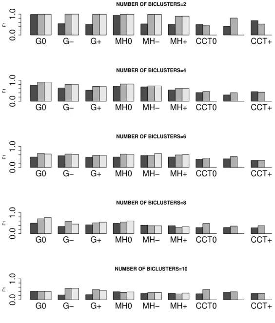
2.3 F1 means for the different models compared. The darker bars cor-respond to the Mixture model, the lighter bars, to the penalized plaid model, and the others to the plaid model. The letter “G” stands for the Gibbs sampler, the letters “MH” for the Metropolis-Hastings algorithm described in this paper, and the letters “CC” in the “CCT” triplet stands for the original method suggested by Cheng and Church to fit a mixture model (darker bars), and the letter “T” for the Turner et al.’s algorithm to fit the plaid model (light bars). The symbol “+” stands for Heavy overlapping in the biclusters; the symbol “-” stands for Moderate overlapping, and the “0” stands for No overlapping. . . . 69

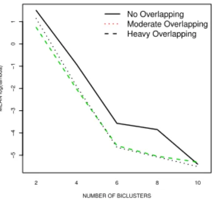
2.4 The profile means of the logarithm of the λ parameter in the pe-nalized plaid model. . . 71

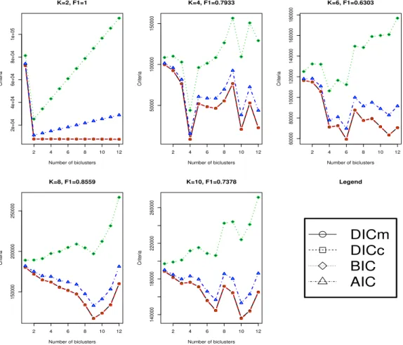
2.5 DICm, DICc, AIC and BIC for the penalized plaid model (p=400,

q=50). The F1 measure refers to the F1 value between the true biclustering and that one associated to the biclustering that

mini-mizes the DICm. The curves for DICmand DICcare overlying. . 72

2.6 DICcand AIC for the Yeast cell cycle data . . . 75

2.7 Biclusters 3, 5, 6, 10, 11 and 13 of the Yeast cell cycle data. The upper subplots correspond to the gene (column) effects, and the right subplots, to the experimental conditions (row) effects. . . . 76

3.1 Examples of simulated data. . . 97

3.2 F1-measure means for the different models compared. The darker bars correspond to the classical plaid model, the red bars, to the algorithm of Cheng and Church, the green bars, to the Bayesian penalized plaid model, and the blue bars, to the Gibbs-plaid model. 99 3.3 AIC and DICc for the Gibbs-plaid model (p=355, q=17). The F1 measure refers to the F1 value between the true biclustering and that one associated to the biclustering that minimizes the DICc. . . 101

3.4 The gene expression levels of the Yeast Cycle data set. . . 103

3.5 AIC and DICcfor the Gibbs-plaid model (p=355, q=17) applied to the Yeast Cycle data set. . . 104

3.6 Yeast Cell Cycle Data. Biclusters 1, 2, and 4 seen at the bottom left corner of the first three images in contrast to the whole data matrix. The rightmost bottom panel corresponds to the original data and the fitted values predicted by the model. . . 105

4.1 BIC for the Colon tumor data . . . 132

4.2 BIC for the SRBCT data . . . 132

4.3 Clustering images for the Colon Tumor data . . . 133

AIC Crit`ere d’information de Akaike ANOVA Analyse de la variance

ARN Acide ribonucl´eique

ARNm Acide ribonucl´eique messager BIC Crit`ere d’information bay´esien Cov Covariance

DIC Crit`ere d’information de d´eviance DNA Acide d´esoxyribonucl´eique

EM Algorithme d’esp´erance-maximisation GO Ontologie des g`enes

ICM Algorithme it´eratif du mode conditionnel IS Importance ´echantillonnale

MCMC Monte Carlo par chaines de Markov MCEM Monte Carlo esp´erance-maximisation

mon ´epouse Eugenie et

J’aimerais exprimer ma profonde gratitude `a mon directeur de th`ese M. Alejandro Murua, pour sa disponibilit´e, son soutien et l’apprentissage continu qu’il a su me dis-penser durant ces ann´ees. Je remercie aussi M. Christian L´eger pour m’avoir incit´e `a venir au D´epartement de math´ematiques et statistique. Merci ´egalement aux professeurs et membres du d´epartement qui ont su m’offrir un cadre tout `a fait propice aux ´etudes et aussi pour leur disponibilit´e. Je ne saurais terminer sans remercier le CRM, l’ISM, le D´epartement de math´ematiques et statistique, la Facult´e des ´etudes sup´erieures et post-doctorales pour leur soutien financier. Enfin, je remercie mes parents, mes fr`eres et soeurs, ma belle famille, mes amis pour leur soutien moral et inconditionnel.

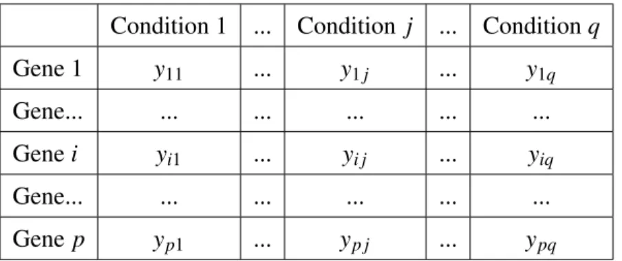
Les donn´ees d’expression g´en´etique obtenues par les technologies micro-puces d’ADN sont une forme de donn´ees g´enomiques `a haut d´ebit. Elles fournissent des me-sures relatives de niveaux d’ARNm (Acide ribonucl´eique messager) pour des milliers de g`enes dans un ´echantillon biologique (Lee et al. [14]). Typiquement, ces donn´ees contiennent un grand nombre (jusqu’`a plusieurs dizaines de milliers) de g`enes, et un nombre d’´echantillons (individus) relativement faible. Ces mesures sont obtenues en immobilisant les g`enes sur des spots dispos´es dans une grille (« array ») sur un support qui est typiquement une lame de verre, une plaquette de quartz, ou une membrane de nylon. `A partir d’un ´echantillon d’int´erˆet, par exemple une biopsie tumorale, l’ARNm est extrait, marqu´e et hybrid´e `a la grille. La mesure de la quantit´e de marques sur chaque spot donne une valeur d’intensit´e qui devrait ˆetre corr´el´ee `a l’abondance du transcrit cor-respondant d’ARN dans l’´echantillon (Huber et al. [10]). La connaissance et l’analyse des donn´ees d’expression g´en´etique peuvent s’av´erer utile dans le diagnostic m´edical, le traitement et la conception de m´edicaments. Ces donn´ees `a micro-puces peuvent ˆetre vues comme une matrice de donn´ees o`u les lignes et les colonnes repr´esentent respecti-vement les g`enes et les conditions ou ´echantillons exp´erimentaux (par exemple : patients, tissus, p´eriodes de temps). Chaque cellule de la matrice est un nombre r´eel et repr´esente le niveau d’expression d’un g`ene sous une condition exp´erimentale.

Une m´ethode standard pour analyser les donn´ees d’expression g´en´etique est le

re-groupement(clustering en anglais) (Kerr et al. [12]) qui peut se faire soit sur les g`enes, soit sur les conditions exp´erimentales. Les techniques de regroupement (k-moyennes : Hartigan et Wong [8], regroupement hi´erarchique : Ward [19], mod`ele bas´e sur le re-groupement : Fraley et Raftery [5]) ont prouv´e leur utilit´e pour comprendre la fonction des g`enes, la r´egulation des g`enes, les processus cellulaires et les sous-types de cellules. Les g`enes co-exprim´es (avec les expressions similaires) peuvent ˆetre group´es ensemble et sont susceptible d’ˆetre impliqu´es dans le mˆeme processus cellulaire (Jiang et al. [11]). Dans un regroupement de g`enes, toutes les conditions exp´erimentales (´echantillons) sont partag´es par toutes les autres grappes. Il en est de mˆeme dans un regroupement de

conditions o`u celles-ci sont group´ees en utilisant tous les g`enes. De plus, les grappes obtenues sont exclusives et exhaustives puisqu’elles forment une partition des g`enes ou des conditions. Cependant, il est bien connu en biologie mol´eculaire qu’un processus cellulaire qui contient un petit sous-ensemble de g`enes peut ˆetre actif seulement dans un sous-ensemble de conditions. En outre, un seul g`ene peut participer `a plusieurs chemins (« pathways ») qui peuvent ou ne peuvent pas ˆetre co-actifs dans toutes les conditions. Ainsi, un g`ene peut donc participer dans plusieurs grappes ou dans rien du tout.

Le bi-regroupement tente de surmonter ces limites de regroupement. La notion de bi-regroupement (ou biclustering en anglais, aussi connu comme co-clustering ou two-way clustering) r´ef`ere au regroupement simultan´e de lignes et de colonnes d’une matrice de donn´ees. Chaque grappe obtenue de ce bi-regroupement sera appel´een bi-grappe

(bi-cluster en anglais) . C’est donc une sous-matrice de la matrice des donn´ees dont les lignes exhibent un comportement similaire `a travers les colonnes et vice versa. Un re-groupement quant `a lui ne peut s’appliquer que sur les lignes, ou sur les colonnes. Un regroupement fournit un mod`ele global tandis que le bi-regroupement donne un mod`ele local. Les lignes ou les colonnes peuvent appartenir `a plusieurs bi-grappes. La bi-grappe peut ˆetre alors imbriqu´ee. La d´etection des bi-grappes imbriqu´ees fournit une meilleure repr´esentation de la r´ealit´e biologique. Le bi-regroupement n’a pas seulement des appli-cations en bioinformatique, il a aussi des appliappli-cations importantes en marketing (Dol-nicar et al. [4]), et dans l’exploration de texte (text-mining, Busygin et al. [2]). Jus-qu’`a r´ecemment, le bi-regroupement n’avait pas rec¸u beaucoup d’attention dans la com-munaut´e statistique. Tr`es peu de mod`eles de bi-regroupement ont ´et´e propos´es dans la litt´erature.

L’objectif de cette th`ese est de trouver des nouvelles m´ethodes qui permettent de s´electionner des bi-grappes dans une matrice de donn´ee. Nous pr´esentons une revue des algorithmes de bi-regroupement qui sont class´es en fonction du type d’imbrication et du type d’homog´en´eit´e. Nous illuminons les mod`eles statistiques sous-jacents `a cer-tains algorithmes populaires. Nous pr´esentons ´egalement deux nouveaux mod`eles de bi-regroupement probabilistes qui sont des extensions du mod`ele `a carreaux (ou plaid) de Lazzeroni et Owen [13]. Le premier mod`ele est un mod`ele `a carreaux p´enalis´e. Il est

bay´esien et contient un param`etre reli´e `a la distribution a priori des ´etiquettes d’apparte-nance des lignes et des colonnes. Ce param`etre contrˆole le niveau d’imbrication entre les bi-grappes et permet de lier les deux algorithmes de bi-regroupement les plus populaires (l’algorithme de Cheng et Church [3] et celui de Lazzeroni et Owen [13]). Les m´ethodes d’´echantillonnage de Gibbs [6] et de Metropolis-Hasting [9] nous permettent d’estimer les bi-grappes. Le second mod`ele est aussi bay´esien et tient compte de l’information a

priorisur les g`enes et les conditions de la matrice d’expression g´en´etique. Cette infor-mation est incorpor´ee `a travers un graphe relationnel par les mod`eles auto-logistiques Besag [1]. L’algorithme de Wang-Landau [18], combin´e avec les m´ethodes de Monte Carlo par chaines de Markov, est utilis´e pour estimer les param`etres. L’utilisation de l’algorithme de Wang-Landau est utile pour contourner l’indisponibilit´e de la constante de normalisation des distributions a priori des ´etiquettes.

Lorsqu’on regroupe les ´echantillons ou les conditions exp´erimentales, le but est de trouver les structures de ph´enotype des conditions qui sont g´en´eralement li´ees `a cer-taines maladies ou `a des effets des m´edicaments. Il a ´et´e d´emontr´e (Golub et al. [7]) que les ph´enotypes d’´echantillons peuvent ˆetre discrimin´es `a travers seulement un petit nombre de g`enes qui ont des niveaux d’expression fortement corr´el´es avec les classes. Ces g`enes sont donc informatifs. Les autres g`enes sont non informatifs (ou bruits) car ils sont consid´er´es non pertinents pour expliquer le regroupement en classes. Il est donc sou-vent n´ecessaire en pratique de s´electionner les g`enes significatifs capables de r´ev´eler la vraie structure du regroupement dans les ´echantillons. Inspir´e du mod`ele `a carreaux, nous pr´esentons un nouveau mod`ele capable de s´electionner les variables dans un contexte de regroupement des donn´ees. Ce mod`ele est reli´e `a ce qui est appel´e dans la litt´erature le mod`ele de m´elange multiplicatif pour le regroupement avec imbrication (Qiang et Ba-nerjee [16]). Il est diff´erent et plus g´en´eral que les mod`eles consid´er´es dans la litt´erature (Pan et Shen [15] et Tadesse et al. [17]) car il permet non seulement l’imbrication entre les grappes, mais aussi, dans chaque grappe, les lignes et les colonnes se comportent de fac¸on similaire (comme dans une bi-grappe `a valeurs coh´erentes sur les lignes et les colonnes). De plus, l’utilisation de la variable latente de s´election de variable dans un algorithme EM de Monte Carlo (Wei et Tanner [20]) semble ˆetre nouveau dans ce

contexte.

Le premier chapitre de cette th`ese introduit le concept de bi-regroupement et pr´esente certains algorithmes en fonction de l’homog´en´eit´e recherch´ee dans les bi-grappes, et le type d’imbrication que l’on peut rencontrer. C’est un chapitre introductif `a la th`ese qui permet de comprendre le bi-regroupement et les approches utilis´ees dans la litt´erature. Il constituera le premier article de cette th`ese intitul´e : « A Survey of Practical Biclustering Methods For Gene Expression Data ». L’autre auteur de cet article est mon superviseur, M. Alejandro Murua, professeur `a l’Universit´e de Montr´eal. La contribution de l’´etudiant dans cet article repose sur la d´erivation des formules, la co-´ecriture du manuscrit et la re-vue de la litt´erature sur les algorithmes de bi-regroupement. Le second chapitre d´ecrit le mod`ele `a carreaux p´enalis´e et les algorithmes reli´es. Il est ´ecrit sous la forme d’un article intitul´e : « The Penalized Plaid model and Related Algorithms ». Cet article a ´et´e sou-mis `a « Journal of Applied Statistics ». L’autre auteur de cet article est ´egalement mon superviseur. Dans ce papier, l’´etudiant a partiellement ´emis des id´ees sur la construction du mod`ele, partiellement d´eriv´e les formules, partiellement conc¸u les exp´eriences sur des donn´ees simul´ees et r´eelles, impl´ement´e et ex´ecut´e les algorithmes, puis co-´ecrit le manuscrit. Le troisi`eme chapitre utilise des champs de Gibbs afin d’introduire de l’in-formation a priori dans le mod`ele `a carreaux. Il est ´ecrit sous forme d’article : « The Gibbs-Plaid Biclustering Model ». Les autres auteurs de cet article sont : Alejandro Mu-rua, professeur `a l’Universit´e de Montr´eal, et Wolfgang Raffelsberger de l’Institut de la g´en´etique et de la biologie mol´eculaire et cellulaire (IGBMC) de l’Universit´e de Stras-bourg, France. L’´etudiant a partiellement ´emis des id´ees sur la construction du mod`ele, partiellement d´eriv´e les formules, propos´e l’algorithme de Wang-landau pour estimer les param`etres, partiellement conc¸u les exp´eriences sur des donn´ees simul´ees et r´eelles, impl´ement´e et ex´ecut´e les algorithmes, puis a co-´ecrit le manuscrit. Le quatri`eme et dernier chapitre pr´esente un mod`ele de s´election de variable dans un contexte de re-groupement de donn´ees. Il est r´edig´e sous forme d’article intitul´e : « Variable Selection With The Plaid Mixture Model For Clustering ». L’autre auteur est mon superviseur Ale-jandro Murua. L’´etudiant a partiellement ´emis des id´ees sur la construction du mod`ele, d´eriv´e les formules, conc¸u l’algorithme EM de Monte Carlo, partiellement conc¸u les

exp´eriences sur des donn´ees simul´ees et r´eelles, impl´ement´e et ex´ecut´e les algorithmes puis a co-´ecrit le manuscrit.

[1] J. Besag. Spatial interaction and the statistical analysis of lattice systems. Journal

of the Royal Statistical Society. Series B (Methodological), 36(2):192–236, 1974. [2] S. Busygin, O. Prokopyev et P. M. Pardalos. Biclustering in data mining.

Compu-ters & Operations Research, 35(9):2964 – 2987, 2008.

[3] Y. Cheng et G.M. Church. Biclustering of expression data. Int. Conf. Intelligent

Systems for Molecular Biology, 12:61–86, 2000.

[4] S. Dolnicar, S. Kaiser, K. Lazarevski et F. Leisch. Biclustering. Journal of Travel

Research, 51(1):41–49, 2012.

[5] C. Fraley et A. E. Raftery. Model-based clustering, discriminant analysis, and density estimation. Journal of the American Statistical Association, 97:611–631, 2000.

[6] S. Geman et D. Geman. Stochastic relaxation, Gibbs distributions, and the Baye-sian restoration of images. IEEE Transactions on Pattern Analysis and Machine

Intelligence, 6(6):721–741, 1984.

[7] T. R. Golub, D. K. Slonim, P. Tamayo, C. Huard, M. Gaasenbeek, J. P. Mesirov, H. Coller, M. L. Loh, J. R. Downing, M. A. Caligiuri, C. D. Bloomfield et E. S. Lander. Molecular classification of cancer : class discovery and class prediction by gene expression monitoring. Science, 286(5439):531–537, 1999.

[8] J. A. Hartigan et M. A. Wong. Algorithm as 136 : A k-means clustering algorithm.

Journal of the Royal Statistical Society. Series C (Applied Statistics), 28(1):100– 108, 1979.

[9] W.K. Hastings. Monte Carlo sampling methods using Markov chains and their applications. Biometrika, 57(1):97–109, 1970.

[10] W. Huber, A. V. Heydebreck et Vingron M. Analysis of microarray gene expression data. Dans in ‘Handbook of Statistical Genetics’, 2nd edn. Wiley, 2003.

[11] D. Jiang, C. Tang et A. Zhang. Cluster analysis for gene expression data : A survey.

IEEE Trans. on Knowl. and Data Eng., 16(11):1370–1386, 2004. ISSN 1041-4347.

[12] G. Kerr, H. J. Ruskin, M. Crane et P. Doolan. Techniques for clustering gene expression data. Comput. Biol. Med., 38(3):283–293, mars 2008. ISSN 0010-4825. [13] L. Lazzeroni et A. Owen. Plaid models for gene expression data. Statistica Sinica,

12:61–86, 2002.

[14] H. K. Lee, A. K. Hsu, J. Sajdak, J. Qin et P. Pavlidis. Coexpression analysis of human genes across many microarray data sets. Genome Research, 14:1085–1094, 2004.

[15] W. Pan et X. Shen. Penalized model-based clustering with application to variable selection. Journal of Machine Learning Research, 8:1145–1164, 2007. ISSN 1532-4435.

[16] F. Qiang et A. Banerjee. Multiplicative mixture models for overlapping clustering. Dans Data Mining, 2008. ICDM ’08. Eighth IEEE International Conference on, pages 791 –796, dec. 2008.

[17] M. G. Tadesse, N. Sha et M. Vannucci. Bayesian variable selection in clustering high-dimensional data. Journal of the American Statistical Association, 100:602– 617, 2005.

[18] F. Wang et D. P. Landau. Efficient, multiple-range random walk algorithm to cal-culate the density of states. Physical Review Letters, 86:2050–2053, Mar 2001. [19] J. H. Ward. Hierarchical groupings to optimize an objective function. Journal

[20] G. C. G. Wei et M. A. Tanner. A Monte Carlo implementation of the EM algo-rithm and the poor man’s data augmentation algoalgo-rithms. Journal of the American

A SURVEY OF PRACTICAL BICLUSTERING METHODS FOR GENE EXPRESSION DATA

1.1 Introduction and notation

With the recent advances in DNA microarray technology and genome sequencing, it has become possible to measure at once gene expression levels of many thousands of genes within a number of different experimental samples or conditions (e.g. different patients, different tissues, or different time points). Data collected with this technology are named gene expression data. They may be of great value in medical diagnosis, treat-ment, and drug design (Wu et al. [37]). Some researchers even claim that the future of medicine lies in this new type of technology. Gene expression data (or microarray data) can be viewed as a data matrix where rows and columns represent genes and experimen-tal conditions respectively. Each matrix entry or cell is a real number, and represents the expression level (profile) of a gene under an experimental condition.

Clustering techniques can be used to group either the genes under all the different experimental conditions or the experimental conditions based on the expressions of all the genes in the data matrix. However, a cellular process may be active only in a subset of conditions and a single gene may participate in multiple cellular processes (Sara and Oliveira [29]). It is therefore highly desirable to move beyond the clustering paradigm, and to develop approaches capable of discovering local patterns (submatrix) in microar-ray data (Ben-Dor et al. [4]).

The data will be represented by a p_{× q matrix Y = (y}i j). In the case of gene

ex-pression data, yi j represents the expression level of the gene i under the experimental

Condition 1 ... Condition j ... Condition q Gene 1 y11 ... y1 j ... y1q Gene... ... ... ... ... ... Gene i yi1 ... yi j ... yiq Gene... ... ... ... ... ... Gene p yp1 ... yp j ... ypq

Table 1.1: Gene expression matrix

Consider K submatrices (or clusters) of the data matrix Y. Letρik= 1 if row i belongs

to the submatrix (or cluster) k, and let it be zero otherwise, k= 1, ..., K. Similarly, let κjk = 1 if column j belongs to submatrix k. and let it be zero otherwise. We will

denote by Ik = {i,ρik = 1} the set of rows in k, and by Jk = { j,κjk = 1}, the set of

columns in k. Their sizes (cardinalities) will be denoted by rk and ck, respectively. Let

¯

y_{· jk}= ∑i∈Ikyi j/rk be the mean of column j in submatrix k, ¯yi·k= ∑j∈Jkyi j/ck, the mean of row i in submatrix k, and ¯yk= ∑_{(i, j)∈k}yi j/rkck, the overall mean of cells in submatrix k.

Clusters versus biclusters

A cluster k of rows is defined as a subset of rows that exhibit a similar behavior across all the columns. Thus, a cluster is a rk× q submatrix of the data matrix Y. Note that one

has in this case r_k= ∑_ip₌₁ρik. A clustering of rows satisfies the following conditions K

∑

∑

since each row must belong to only one cluster, and each cluster must contain all the columns (see Figure 1.1). Similarly, a cluster k of columns is defined as a subset of columns that exhibit a similar behavior across all rows. A column cluster is then a p_×ck

of columns satisfies the following conditions K

∑

∑

since each cluster must contain all rows, and each column must belong to only one cluster (see Figure 1.2). However, a bicluster k is a subset of rows that exhibit similar behavior across a subset of columns, and conversely (see Figure 1.3). A bicluster is a

rk× cksubmatrix of the data matrix Y. It satisfies

0_≤ K

∑

∑

since each row (or column) may belong to several biclusters (see Figure 1.3). Rows clusters Figure 1.1: Clustering of rows Columns clusters Figure 1.2: Clustering of columns Biclusters Figure 1.3: Biclustering of the matrix data

The problem of biclustering consists of finding a possibly overlapping partition of blocks (biclusters) of the data matrix. The main unknown parameters of biclustering are, as in the case of clustering, the number of biclusters K, and the row and column membership labels(ρ,κ_{) = {(}ρik,κjk)}, i = 1,... p, j = 1,...,q, k = 1,...K. Note that contrary to

clustering, biclustering involves two sets of unknown labels. As in any clustering model, each bicluster k must satisfy a predetermined specific characteristic of homogeneity. Sara and Oliveira [29] gave a somewhat thorough review of popular biclustering

tech-niques. They analyzed and classified a large number of existing approaches according to the type of homogeneity defining biclusters. They identified four types of homogeneity: biclusters with constant values, biclusters with constant values on rows or columns, bi-clusters with coherent values, and bibi-clusters with coherent evolution. In Section 1.2, we give the definitions and some examples of each type of homogeneity.

Another key difference between clustering and biclustering is the concept of

over-lapping between the clusters (or biclusters). We say that a bicluster k1 overlaps with

another bicluster k2if these two biclusters share some rows or some columns of the data

matrix. From this definition, we can find in the literature three types of overlapping. The first one is the row or column overlapping. Only the rows (or the columns) can belong to more than one bicluster. The second one is the Row-column overlapping. Both rows and columns may belong to several biclusters, but a cell in the matrix cannot belong to more than one bicluster. The third and last type of overlapping is the cell overlapping which is more general than the others. A cell (a specific row and column) may belong to several biclusters. In Section 1.3 we survey some of the biclustering models and algorithms that have been developed for gene expression analysis for each type of overlapping. Our list of algorithms is not exhaustive, but it rather focuses on what we believe are the more practical methods.

1.2 Types of biclusters

In this section we follow closely the exposition of Sara and Oliveira [29].

1.2.1 Biclusters with constant values

A bicluster with constant values is a submatrix whose cells share a common value. In the case of gene expression data, constant biclusters are subsets of genes with simi-lar expression values within a subset of conditions. A perfect constant bicluster verifies

yi j =µk for all(i, j) ∈ k. The values yi j found in a constant bicluster can be written as: yi j =µk+εi j whereεi j is a noise associated to yi j. Table 1.2 gives an example of this

12 12 12 12

12 12 12 12

12 12 12 12

Table 1.2: Bicluster with constant values

Hartigan [16] seems to be the first to have applied a clustering method to simultane-ously cluster rows and columns. He introduced a partition-based algorithm called direct

clusteringthat allows the division of the data in submatrices (biclusters). The quality of a bicluster was evaluated by the sum of squared errors

∑

(i, j)∈k

(yi j− ¯yk)2. (1.4)

Hartigan’s algorithm stops when the data matrix is partitioned into the desired number of biclusters, say K. The quality of the partition is evaluated by the total sum of squared errors SSQ= K

∑

∑

Tibshirani et al. [33] and Cho et al. [10] have also used (1.4) as a measure of biclustering quality to find constant biclusters.

1.2.2 Biclusters with constant values on rows or columns

This type of bicluster exhibits coherent values either on the columns or the rows. The biclusters in Tables 1.3 and 1.4 are examples of perfect biclusters with constant rows and columns, respectively.

12 12 12 12

14 14 14 14

9 9 9 9

Table 1.3: Constant values on rows

12 7 10 11

12 7 10 11

12 7 10 11

Table 1.4: Constant values on columns A perfect bicluster with constant values on rows is a submatrix k where all the values

in the bicluster can be obtained using one of the following expressions:

yi j =µk+αik or yi j =µk×αik, (1.5)

whereµkis the typical value in the bicluster,αikis the adjustment (additive or

multiplica-tive) for row i. A perfect bicluster with constant values on columns is defined similarly. A direct approach to identify this type of bicluster is to first do a normalization on the rows or columns using the mean sample of the rows and of the columns, respectively, and then, apply a method to find biclusters with constant values. Sheng et al. [31] and Segal et al. [30] introduced a probabilistic model to find biclusters with constant values on columns (see Sections 1.3.1 and 1.3.3 for more details).

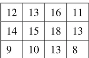
1.2.3 Biclusters with coherent values

A bicluster with coherent values both on rows and columns is an improvement over the types considered previously. A perfect bicluster k is defined as a subset of rows and a subset of columns verifying for all_{(i, j) ∈ k:}

yi j =µk+αik+βjk or yi j =µk×αik×βjk, (1.6)

whereµk is the typical value of the bicluster,αik is the adjustment for row i, andβjk is

the adjustment for column j. This type of homogeneity is very common in the literature and many authors (Cheng and Church [9], Lazzeroni and Owen [20], Gu and Liu [14], Zhang [39], Turner et al. [34], Cho et al. [10], Chekouo and Murua [7], Hochreiter et al. [17], Lee et al. [21]) have used it. Note that when an additive model is assumed in a bicluster k, the residual of yi j is ri jk = yi j− ¯yi·k− ¯y· jk+ ¯yk and ri jk = 0 if and only

if yi j = µk+αik+βjk. The particular cases of αik = 0 (or αik = 1) and βjk = 0 (or

βjk= 1) in the model given by expression (1.6) give the biclusters with constant values

on columns and with constant values on rows, respectively. Tables 1.5 and 1.6 illustrate examples of an additive and a multiplicative model, respectively.

12 13 16 11

14 15 18 13

9 10 13 8

Table 1.5: Additive coherent values

12 24 6 18

10 20 5 15

1 2 0.5 1.5

Table 1.6: Multiplicative coherent values

1.2.4 Biclusters with coherent evolution

Ben-Dor et al. [4] have defined a bicluster as a submatrix preserving an order (OPSM). A submatrix preserves an order if there exists a permutation of its columns so that the sequence of values in each row is strictly increasing. An example of this type of bicluster is shown in Table 1.7. In the case of gene expression data, these biclusters correspond to subsets of genes and conditions such that the expression levels of all the genes have a same linear order across the conditions. Ben-Dor et al. [4] defined a complete model of OPSM as being a couple (T,π) where T is a set of s columns and π = (t1, ...,ts) is

a linear order on T . In this model, a row i is said to support(T,π_{) if {y}it1, yit2, . . . , yits} is an increasing sequence. Their algorithm look for a complete maximal set in terms of rows.

12 8 10 9

15 11 14 13

32 7 20 10

Table 1.7: Bicluster with coherent evolution

1.3 Types of overlapping

1.3.1 Row or column overlapping methods

In this section, we will review some methods which look for biclusters with over-lapping only between rows, or only between columns. In terms of labels, this type of biclustering can be characterized by ∑K_k=1ρik≥ 1 for row overlapping, or ∑Kk=1κjk≥ 1

for column overlapping. Figures 1.4 and 1.5 illustrate the row overlapping and the col-umn overlapping models, respectively.

Figure 1.4:Row overlapping model Figure 1.5:Column overlapping model Tang et al. [32] applied an unsupervised approach for gene expression data analy-sis called Interrelated Two-Way Clustering (ITWC) to find biclusters with possible row (gene) overlapping. Their goal was to find important gene patterns, and at the same time perform cluster discovery on the experimental conditions. This is equivalent to variable selection (selection of genes) in the context of conditions clustering. There are five steps within each iteration of ITWC. The first step consists of clustering the rows of the ma-trix into two clusters G1and G2using k-means. In the second step, based on each gene

group Gi, i = 1, 2, the columns (conditions) are clustered into two clusters Si,1 and Si,2.

The third step combines these clusters to form four groups of columns C1= S1,1∩ S2,1, C2= S1,1∩ S2,2, C3= S1,2∩ S2,1 and C4= S1,2∩ S2,2. A pair of groups(Cs,Ct) is said to

be a heterogeneous pair if the groups do not share columns, i.e., for all u_{∈ C}s, v∈ Ct, if u_{∈ S}i, j1 and v∈ Si, j2, then j16= j2. The fourth step of ITWC consists of finding

hetero-geneous pairs(Cs,Ct), s,t = 1, . . . , 4. The vector-cosine similarity between two vectors u= (u1, ..., uq) and v = (v1, ..., vq) is given by:

cos(u, v) = ∑ q j=1ujvj q ∑q_j=1u2_jq∑q_j=1v2_j .

The fifth step sorts the rows in descending order according to the sum of vector-cosine similarities between each row and the two occupancy patterns associated with each

het-erogeneous pair. The two occupancy patterns for a hethet-erogeneous pair(Cs,Ct) are

ob-tained by setting all components corresponding to columns in Cr to one, and setting

all remaining columns to zero, r_{∈ {s,t}. The number of rows are reduced by keeping} only the first 1/3 of the sorted rows from each heterogeneous pair. Leave-one-out cross-validation is used to evaluate the prediction performance of the partition so obtained. These five steps are repeated using the selected rows until a predetermined stopping criterion is satisfied. For example, until the occupancy ratio between columns in the heterogeneous groups and all conditions,_(|Cs| + |Ct|)/q, is maximized.

Gu and Liu [14] develop a Bayesian approach to find biclusters assuming that the only possible overlapping is between the experimental conditions (columns). The priors of the labelsρ andκ are set to respect this restriction. Their model, which is based on the plaid model, may be written as follows

yi j= K

∑

∑

whereεi jkis the noise term for cluster k, and ei j models the data points that do not belong

to any cluster. From this expression, Gui and Liu derive the marginal distribution of Y given the labels. Inference is based on Markov chain Monte Carlo (MCMC) sampling. The number of biclusters is selected according to the Bayesian information criterion (BIC).

Sheng et al. [31] also develop a biclustering method where the overlapping is only allowed between the columns. Their method proposes a Bayesian framework and works on discrete data. In this model, the columns belonging to any determined bicluster fol-low independent multinomial distributions. Thus, these biclusters have constant values on columns. Sheng et al. use a Gibbs sampling to sample from the gene/column mem-bership labels. In order to find several biclusters, the authors choose to mask the genes selected in previous biclusters, so as to run again the same algorithm on the remaining data. By doing this, only the columns can be selected more than once.

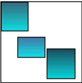
1.3.2 Row-column overlapping methods

These methods aim at finding biclusters where rows or columns (but not a cell) may belong to more than one bicluster. They may be characterized as satisfying ∑Kk=1ρikκjk≤

1. They may also satisfy ∑K_k=1ρik≥ 1 or ∑Kk=1κjk ≥ 1, i = 1,..., p, j = 1,...,q. This

type of biclustering may be further characterized by the type of pattern or structure found in the data matrix which may be checkerboard-like or not.

Figure 1.6:Checkerboard structure Figure 1.7: Non-checkerboard structure

1.3.2.1 Checkerboard structure

A particular type of row-column overlapping is given by assuming a checkerboard structure in the data matrix. Models requiring this structure allow for the existence of K = ML non-exclusive biclusters, where each row belongs to exactly M biclusters, and each column belongs exactly to L biclusters. Figure 1.6 shows an example of this structure for M= L = 3.

Cho et al. [10] have developed an algorithm that simultaneously discovers clusters of rows and columns while monotonically decreasing the corresponding sum of squared residuals. Their optimization problems consists of minimizing the total sum of squared residuals given by

K

∑

k=1

rkckHk,

with Hk = ∑_{(i, j)∈k}(yi j− ¯yi·k− ¯y· jk+ ¯yk)2/rkck. In what follows, we show that this

associated statistical model. Given the set of parametersθ = (µ,α,β,σ2_{), the}

underly-ing model of Cho et al. [10] could be written as

P_(Y|θ,ρ,κ_{) ∝ exp(−} 1 2σ2

∑

∑

where ∑Mm=1ρim= ∑L_l=1κjl= 1. The membership labelsρimandκjl are the membership

labels associated with the clustering of the rows and the columns, respectively. This model assumes the same variance distribution in all K biclusters. If we further assume a uniform distribution as the prior distribution on the labels, i.e.,

p(ρim= 1) = p(ρim= 1,ρim′= 0, m′6= m) = 1 M for all i, m p(κjl= 1) = p(κjl= 1,κjl′= 0, l′6= l) = 1 L for all j, l

then, applying the hard EM algorithm on the complete distribution P(y,ρ,κ_|θ) under the usual constraints of identifiability onα andβ, yield the following parameter estimates at each EM iteration

ˆ

µml = ¯yk, αˆiml = ¯yi·k− ¯yk, βˆjml= ¯y· jk− ¯yk, and ˆσ2=

1 pq K

∑

For the labels, given these estimators, we have

pim = p(ρim= 1,ρim′= 0, m′6= m|y,Θ−ρ) ∝ exp ( − 1 2σ2

∑

cluster m with the highest probability, i.e.,

ρim= 1 if and only if m = arg max m pim = arg min m

∑

∑

(yi j− ¯yi·k− ¯y· jk+ ¯yk)2. (1.8)

Similarly,

κjl= 1 if and only if l = arg min

l

∑

∑

i_∈Im,k=(m,l)

(yi j− ¯yi·k− ¯y· jk+ ¯yk)2. (1.9)

Relations (1.8) and (1.9) are exactly the same relations that Cho et al. [10] have used to update the labels without explicitly writing a model for the data.

Another work which assumes the checkerboard structure is that of Govaert and Nadif [13]. They refer to their biclustering model as block clustering. In contrast to Cho et al. [10], Govaert and Nadif assume that the prior probabilities on the membership labels are also parameters of interest to be estimated. They also used a hard EM algorithm, the Classification EM (CEM) algorithm, to simultaneously cluster the rows and the columns. Their block mixture model is given by

P_(y|θ) =

_∑

∏

∏

∏

whereφi j(yi j;µlm) is a probability density parametrized byµlm. The parameters pl and qmare the probabilities that a row and a column belong to the l-th and m-th component,

respectively. The parameterθ in this model is the vector(p1, ..., pM, q1, ..., qL,µ11, ...,µLM).

Kluger et al. [19] introduce a biclustering technique called spectral biclustering. It uses a singular value decomposition to identify bicluster structures in the data. This method assumes that the expression matrix Y has a checkerboard-like structure. By ap-plying the singular value decomposition on Y, one finds the eigenvectors of YYT and YTY. Note that if v is an eigenvector of YYT, then YTv is an eigenvector of YTY. For any eigenvector pair (v, YT_{v), we check whether each of the eigenvectors can be}

deter-mine whether the data have a checkerboard pattern. For that, the authors use a one-dimensional k-means algorithm to test this fit. Kluger et al.’s assume a multiplicative model, that is, the expression level of a specific gene i in a condition j can be expressed as a product of three independent factors. The first factor is called the hidden base

ex-pression level Ei j (i.e., µ). The entries of E within each block are constant. The second

factor represents the genes’ expression tendencies across different conditions (α). The last factor represents the role of particular conditions over the genes’ expression tenden-cies (β). The goal is to find the underlying block structure of E. For that purpose, the rows and the columns are first normalized. Let R and C denote the diagonal matrices

R= diag(Y1p) where 1p= (1, .., 1) ∈ Rp, and C= diag(1TpY). The block structure of E

is now reflected in the stepwise structure of pairs of eigenvectors with the same eigenval-ues of the normalized matrices M= R−1YC−1YT _{and M}T_{. Theses two eigenvalue}

prob-lems can be solved through a standard singular value decomposition of R−1/2YC−1/2.

1.3.2.2 Non-checkerboard structure

Figure 1.7 shows an example of this structure with K = 3. The algorithm of Cheng and Church [9], one of the most popular biclustering algorithms, falls in this category. Cheng and Church seem to be the first authors to have introduced the term biclustering in the literature. In their algorithm, the mean squared residual H_kplays a crucial role as a measure of coherence of the rows and columns in a bicluster. Letδ > 0. A sub-matrix k is said to be aδ-bicluster if Hk<δ. Cheng and Church’s algorithm aims at finding large

and maximal biclusters with scores below a certain predetermined small threshold δ. Cheng and Church suggest a greedy heuristic search so as to rapidly converge to a locally maximalδ-bicluster. A single row or column deletion step iteratively removes the row or column that gives the maximum decrease in H_k. A multiple row or column deletion step follows the same idea, but this time it removes multiple rows or columns in a single iteration. A row or column addition step adds to a given bicluster rows and columns that do not increase the actual score of the bicluster. The general algorithm is composed of a row or column deletion followed by a row or column addition in each iteration. The biclusters are found one at a time. Once a bicluster is found, its rows and columns are

masked with uniform random numbers. The process is repeated until K biclusters are found. The masking procedure renders the overlapping between the biclusters unlikely. Cheng and Church justify their algorithm based on the two following assertions.

Assertion 1. The set of rows that can be completely or partially removed with the net

effect of decreasing the score of a bicluster k is:

R1=

(

i_{∈ I}k,

1

ck _j

∑

(yi j− ¯yi_·k− ¯y_{· jk}+ ¯yk)2> Hk

)

. (1.10)

Assertion 2. The set of rows that can be completely or partially added with the net effect

of decreasing the score of a bicluster k is:

R2= ( i_{∈ I}/ k, 1 c_{k j}

∑

(yi j− ¯yi·k− ¯y· jk+ ¯yk)2< Hk

)

. (1.11)

Chekouo and Murua [7] have attempted to mimic Cheng and Church’ algorithm within a Bayesian framework. They define the underlying model in Cheng and Church’s algorithm as a model similar to the one given by the expression (1.7) of Gu and Liu [14]. However, contrary to (1.7), Chekouo and Murua’s model assumes the possibility of having row or column overlapping in the same biclustering. In fact, the labels satisfy ∑K_k=1ρikκjk ≤ 1 for all i, j. The prior on the labels is a double-exponential-like

distri-bution with a large inverse scale (penalty) parameter (see Section 1.3.3 below for more details). Chekouo and Murua were successful in showing that both assertions 1 and 2 may be derived as updating proposal movements in a Metropolis-Hastings procedure. Consequently, using these assertions in a MCMC sampler will lead to estimates of the posterior labels.

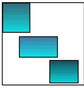
1.3.3 Cell overlapping methods

In this section, we present biclustering methods that allow general overlapping be-tween biclusters, i.e., where each cell(i, j) of the data matrix may belong to more than one bicluster. These methods may be characterized by the condition ∑Kk=1ρikκjk > 1.

The biclusters in this biclustering are arbitrarily positioned in the matrix. Figure 1.3 shows an example of this type of biclustering.

1.3.3.1 Additive models

One of the most popular models that takes into account this structure is the plaid

modelof Lazzeroni and Owen [20] which is defined by

yi j ∼ Normal µ0+ K

∑

The general biclustering problem is now formulated as finding parameter values so that the resulting matrix would fit the original data as much as possible. Formally, the prob-lem consists of minimizing

p

∑

∑

∑

under the constraints: ∑_ip₌₁αikρik = ∑qj=1βjkκj= 0 for all k. A layer is a bicluster in

the sense of Cheng and Church [9]. A plaid is an ensemble of additive layers. Lazzeroni and Owen propose to minimize (1.13) by using an iterative heuristic algorithm. New layers are added to the model one at a time. To simplify the description of their method, suppose that we already know K_{− 1 layers, and that we seek to uncover the K-th layer.} Letµi jk=µk+αik+βjkand Zi jK= yi j−µi j0−∑K_k=1−1µi jkρikκjkthe residual from the first K_{− 1 layers. We need to minimize}

Q=1 2 p

∑

∑

subject to the above identifiability constraints onαiK andβjK.

The proposed method to solve (1.14) is again iterative. A relaxation in the parameters is introduced to simplify the optimization problem. The binary latent variablesρik,κjk

constraints: ∑_ip₌₁αiKρiK2 = ∑ q

j=1βjKκ2jK = 0.

The hard-EM estimators given in the previous sections are similar to those of Lazze-roni and Owen with no relaxation. With the relaxed parameters, the updates ¯ρiK and ¯κjK

are given by ¯ ρik = ∑jµi jKκjkZi jK ∑jµi jK2 κ2jK , (1.15) ¯ κjk = ∑iµi jKρikZi jK ∑iµi jK2 ρiK2 . (1.16)

The importance of layer k is measured by σ2 k = ∑

p i=1∑

q

j=1ρikκjkµ_{i jk}2 . A layer is

accepted if its importance is significantly larger than what would be found in noise Zi j.

For a set of K layers, the algorithm allows to re-estimate all of the µi jk, by cycling

through k = 1, .., K several times. These backfitting cycles only conduct a partial re-optimization, since the updating is done only on all the µi jk parameters, but not on the

labelsρ andκ parameters, which are kept as known values after the last layer has been found.

The most successful starting values have been found using a singular value decom-position on Z. Theρandκvectors are initialized as the eigenvectors associated with the largest singular values. This choice was motivated by the updating equations forρ and κ (equations (1.15) and (1.16)) whenµi jk= 1.

Segal et al. [30] also assumed an additive model. This is given by

yi j∼i.i.dNormal µ0+ K

∑

Note that each column belongs to all the biclusters as in clustering. However, this model allows for the overlapping of layers. Contrary to the work of Lazzeroni and Owen [20], the model of Segal et al. [30] does not consider row effects αik, and the variances may

be column-dependent. It is easily shown (see Chekouo and Murua [8]) that this model is similar to the multiplicative mixture model for overlapping clustering (Qiang and

Baner-jee [24]). The authors referred to this model’s biclusters as processes. The prior distribu-tions forβjk andρik are assumed to be independent uniforms (over some appropriately

bounded range) and binomials, respectively. All the parameters are estimated using a hard EM algorithm as follows:

1. Initialize the labelsρusing a classical method of clustering (k-means for example). 2. (hard E-Step) Repeat (a) and (b) until convergence:

(a) Find theβjk that maximizes its full conditional distribution.

(b) Find theρikthat maximizes its full conditional distribution.

3. Estimate the parameters qik= P(ρik= 1) (M-step).

Turner et al. [34] propose an improved biclustering of microarray data using the plaid model. They also propose a different algorithm for fitting the plaid model. Their ap-proach uses binary least squares (i.e., hard EM algorithm) to update the cluster mem-bership parameters. This somewhat simplifies the updating of the other parameters. The

backfittingis done as in the case of Lazzeroni and Owen [20].

Zhang [39] proposes a hierarchical Bayesian version of the plaid model. He provides an empirical Bayes algorithm for sampling the posteriors in two steps. In the first step, he estimates the membership labels by maximizing their marginal posteriors. During the second step, he directly calculates the Bayesian estimates for the other parameters given the values of the membership labels. To improve the overall estimation, he runs

backfittingto update the parametersΘk = (µk,αik,βjk,ρik,κjk,σ2) given Θt, t6= k. The

backfitting is performed after having done a greedy search for the K layers, as in the case of Lazzeroni and Owen [20].

Chekouo and Murua [7] generalize the plaid model also within a Bayesian frame-work. They introduce a modified extended version of the Bayesian plaid model. The au-thors refer to this model as the penalized plaid model. It aims at controlling the amount of bicluster overlapping by considering a penalization on the amount of overlapping. This is carried out by the introduction of a so-called penalty parameter which will be

denoted byλ. The model fully accounts for a general overlapping structure, as opposed to just a one dimensional (row or column) overlapping as in the model of Gu and Liu [14]. The parameters are determined by an MCMC sampler all at once as opposed to the sequential greedy search algorithm of Zhang [39]. The model also takes into account the problem of identifiability of the row and column effects. As in ANOVA, it assumes that the sum of these effects vanishes within each bicluster. In addition, the penalized plaid model may be seen as a continuous extension of the non-overlapping model of Cheng and Church [9] to the plaid model. Formally, given all the parameters,

yi j ∼i.i.dNormal µ0γi j+ K

∑

whereγi j = ∏k(1 −ρikκjk) is the label associated with the zero-bicluster, i.e., a cluster

containing some observations which are not well explained by the main biclusters; and µ0is the mean of the zero-bicluster. Note that when ∑K_k=1ρikκjk≤ 1 andσ2(ρi,κj) =σ_k2

depends of bicluster k, the model becomes the underlying model of Cheng and Church. But when ∑K_k=1ρikκjk is allowed to become larger than 1, and σ2(ρi,κj) =σ2 is

con-stant, the model becomes the plaid model introduced by Lazzeroni and Owen.

The prior distribution on the labels is defined by a discrete double-exponential with scale parameterλ π((ρ,κ_)|λ) ∝ exp ( −λ

_∑

∑

The scaleλ _{≥ 0 may be viewed as a penalty parameter that controls the amount of} bi-clustering overlapping. Ifλ = 0, the labels are a priori uniformly distributed (e.g., as in the original plaid model). There is no constraint on the structure of the overlapping (i.e., there is cell overlapping). Whenλ _{→ ∞ , the model becomes the row-column} overlap-ping model of Cheng and Church. Chekouo and Murua show via a simulation study that the logarithm of the posterior mean of λ decreases nearly linearly with the number of biclusters and the amount of overlapping in them. They argue that the penalty parameter λ may serve as a measure of complexity of the data. In order to choose an appropriate

number of biclusters, they suggest using a modified version of the deviance informa-tion criterion (DIC). The modified DIC is based on the condiinforma-tional distribuinforma-tion given the membership labels, and on the maximum a posteriori (MAP) estimators of the param-eters. We note that this work appears to be one of the first to have properly addressed the model selection (i.e., the choice of number of biclusters) problem within the context of biclustering. Their work also demonstrates that the use of Bayesian computational techniques such as the Gibbs sampler and Metropolis-Hastings algorithm to estimate the biclustering yield far better results than hard-EM or Iterated Conditional Modes (ICM), and ad hoc heuristic techniques.

1.3.3.2 Informative priors

In another paper, Chekouo and Murua [6] propose a model that takes into account prior information on genes and conditions through pairwise interactions. Their model is a Gaussian plaid model for biclustering combined with a discrete Gibbs field or au-tologistic distribution (Besag [5], Winkler [36]) that conveys the prior information. The Gibbs field prior is a model for dedicated relational graphs, one for the genes and an-other for the conditions, whose nodes correspond to genes (or conditions) and edges to gene (or condition) similarities. Each relational graph is provided with a neighborhood structure. The notation i_{∼ i}′ will denote that nodes i and i′ in the graph are connected with a graph edge, i.e., the relation i_{∼ i}′is satisfied if and only if i and i′are neighbors. Each edge is assigned a weight. For the gene graph, the weights are given by

Bii′(Tρ,σρ) = 1 Tρ exp − 1 2σ2 ρ dρ(i, i′)2 ! .

where Tρ and σρ are the temperature and kernel bandwidth parameters of the graph,

respectively. The “distances” dρ(i, i′) are induced by genes similarities based on the en-tropy information (Resnik [26]) extracted from GO (Gene Ontology) annotations (Ash-burner et al. [1]). The prior for the gene labels ρk is given by the binary Gibbs random