ÉCOLE DE TECHNOLOGIE SUPÉRIEURE UNIVERSITÉ DU QUÉBEC
THESIS PRESENTED TO
ÉCOLE DE TECHNOLOGIE SUPÉRIEURE
IN PARTIAL FULFILLMENT OF THE REQUIREMENTS FOR A MASTER’S DEGREE WITH THESIS IN ENVIRONMENTAL ENGINEERING
M.Sc.A.
by
Émilie BOUCHARD
CHARACTERIZATION OF HYDROLOGICAL PROCESSES OF A GLACIARIZED WATERSHED CATCHMENT IN CANADIAN ST. ELIAS MOUNTAINS USING
NATURAL TRACERS
MONTREAL, OCTOBER 17TH, 2016
This Creative Commons licence allows readers to download this work and share it with others as long as the author is credited. The content of this work may not be modified in any way or used commercially.
BOARD OF EXAMINERS (THESIS M.SC.A.)
THIS THESIS HAS BEEN EVALUATED BY THE FOLLOWING BOARD OF EXAMINERS
M. Michel Baraër, Thesis Supervisor
Département du génie de la construction at École de technologie supérieure
M. Jean-Sébastien Dubé , Chair, Board of Examiners
Départment du génie de la construction at École de technologie supérieure
M. Jeffrey McKenzie, Member of the jury
Earth and Planetary Sciences Department at McGill University
THIS THESIS WAS PRENSENTED AND DEFENDED
IN THE PRESENCE OF A BOARD OF EXAMINERS AND THE PUBLIC MONTREAL, OCTOBER 4TH, 2016
ACKNOWLEDGMENTS
I will do my best to mention all of those whose support contributed to the success of this research project and whose academic or moral support was crucial to this paper. I cannot possibly name everybody, those unnamed I would like to use this opportunity to thank you.
Initially, I would like to thank my project supervisor, Michel Baraër, without whom none of this would have been possible. I was lucky to walk into your office that day and I am grateful you took that chance on me. Thank you for your patience, your undivided attention, and your moral and academic support. It was truly a pleasure to work with you, a grand adventure I am always going to talk about. I am forever thankful for the opportunity I had to work under your supervision.
To Anna, I don’t know what I would have done without you. Thank you for always asking the right questions and taking the time to help me when I needed it, and for your guidance into this world of glaciology I knew nothing about. I am grateful to call you a friend and I will always cherish the times we spent together. Thank you for sharing your passion with me, this project wouldn’t have been the same without you.
I would like to thank everyone at the DRAME for the academic and moral support you have shown me all along this project. It was a pleasure working with you, Jean-Luc, Mélissa, Soudabeh, Martine, Mariana, Pierre-Luc, Richard, Magali, Alex and Salam.
Of a course my entire family for showing your support and help during this project, grand-parents, aunts and uncles, as well as all the cousins I am lucky to have. Tante Lyne thank you for always thinking of me and my well-being. Tante Élise, you were indispensable in the realisation of this project in so many ways. Nanny, thank you for being there for me anytime of the day or night. And a special thanks to all my cousins for their smiles and interests and the fun we’ve had reconnecting!
To my sister and my brother, Alex and Félix, you always know how to bring back my smile and give me some confidence. You will eternally be the best friends and the greatest supporters I have.
I would also like to thank the friends along the way that helped me directly or indirectly with this project: Alex, Anna, Vic, Eric, Michaël, Sam, K’èdukà, Jessica, Scott and Daniel. Thank you so much. To Mel, thank you for the endless hours of moral support and relief you gave me. Thank you Guillaume for all the patience and support you’ve shown me, I am thankful for all the precious moments spent together.
This last one goes to the most important people, without whom I wouldn’t be here today, maman et papa. Merci de m’avoir donné le meilleur de vous, d’avoir su m’encourager et de n’avoir jamais arrêté de croire en moi. Maman, merci pour ton support, tes conseils et ta sagesse. Papa, merci de toujours m’aider dans mes projets d’école, encore aujourd’hui, ton assurance est toujours réconfortante. Vous resterez tous les deux des modèles exemplaires à suivre.
CHARACTERIZATION OF HYDROLOGICAL PROCESSES OF A GLACIARIZED WATERSHED CATCHMENT IN CANADIAN ST. ELIAS MOUNTAINS USING
NATURAL TRACERS Émilie BOUCHARD
RÉSUMÉ
Dans plusieurs régions du monde, des changements dans les processus hydrologiques des bassins versant glaciaires alpins ont été noté; ceux-ci ont un impact important sur les ressources en eau et peuvent affecter les écosystèmes et les populations en aval. Les bassins subarctiques tels que ceux trouvés dans le sud du Yukon (Canada) sont particulièrement sensibles aux changements hydrologiques liés au climat. Pour mieux comprendre l’évolution et l’impact de ces changements sur les systèmes hydrologiques subarctiques, nous avons porté enquête dans la chaîne de montagne Saint-Elias au Yukon en utilisant les traceurs hydrochimiques naturels pour interpréter les contributions glaciaires. Notre site d’étude est un petit bassin versant qui se verse dans la partie supérieure du bassin versant Duke, la vallée ainsi surnommée B contient trois glaciers numérotés de B1 à B3 du plus grand au plus petit. L’objectifs principal était d’identifier les sources d’eau en utilisant les signatures hydrochimiques distinctes de chacune, ainsi que déterminer leurs contributions relatives au volume total à l’exutoire du bassin. La méthode a aussi été utilisée pour identifier les contributions relatives au cours du cycle diurne.
Durant l’été 2015, un échantillonnage centralisé sur le bassin B a donné lieu une analyse spatiale pour les trois glaciers et une analyse temporelle du bassin entier. Les échantillons ont été analysés pour le carbone organique, les ions principaux et les isotopes stables lourds de l’eau (δ18O and δ2H). L’ensemble de données a été soumis à des méthodes statistiques et
au modèle de mélange du hydrochemical basin characterization method (HBCM) pour les analyses qualitative et quantitative. Les contributeurs ont été séparés à l’aide du pH, la conductivité électrique et les concentrations de potassium, magnésium et sulfate
Les résultats montrent que durant la période d’échantillonnage la majorité du volume d’eau provient des eaux de fonte avec une quantité négligeable des sources souterraines telles que les moraines. Le glacier B1 contribue la majorité du volume total (59,43% - 69,06%) dépendamment des conditions externes telles que la température et la radiation solaire. L’utilisation de HBCM sur l’échantillonnage du cycle diurne a montré des résultats positifs en séparation glaciaire, mais la méthode reste expérimentale, par contre son succès dans le bassin B démontre une forte possibilité de réussite pour la caractérisation du bassin Duke entier.
CHARACTERIZATION OF HYDROLOGICAL PROCESSES OF A GLACIARIZED WATERSHED CATCHMENT IN CANADIAN ST. ELIAS MOUNTAINS USING
NATURAL TRACERS Émilie BOUCHARD
ABSTRACT
Changes in the hydrological processes of alpine glacierized watersheds have been observed in most regions of the world. These have an important impact on water resources and can affect downstream ecosystems and populations. Subarctic catchments such as those found in southern Yukon (Canada) are particularly sensitive to climate related hydrological changes. To further understand the ongoing evolution of subarctic hydrological systems, we applied natural tracers based investigations in the Saint-Elias mountain range of the Yukon. Our study site consisted of a small watershed, named B for logistical reasons, of the upper Duke watershed. B watershed contains three small glaciers numbered B1 to B3 from largest to smallest.
The main goal was to identify water sources using hydrochemical signatures and their relative contributions to outflows in the catchment as well as using the method to identify sources contributing during the diurnal cycle.
During the summer of 2015, extensive sampling of watershed B resulted on a spatial analysis of all three glaciers and a temporal analysis on the entire watershed. Samples were analyzed for organic carbon, major ions and heavy stable water isotopes (δ18O and δ2H). The resulting
dataset was then processed using statistical methods and the hydrochemical basin characterization method (HBCM) for a qualitative and quantitative analysis. In this study, end-members were separated using pH, electrical conductivity, potassium, magnesium and sulfate concentrations.
Results show that on the sampling period, watershed outflows consisted mainly of glacier meltwater with a non-negligible contribution of other water sources such as ice-cored moraines. B1 glacier was found contributing 59.43% at low temperature and radiation and 69.06% during a high temperature and radiation day, while inversely B2 and B3 combined contribution were 35.66% and 29.89% during those days. The use of HBCM on samples collected over the diurnal cycle was an experimental approach; it showed positive results separating glacial and non-glacial sources.
The HBCM proved to be successful in the B valley, and therefore present a high possibility of success for the hydrochemical characterization of the entire upper Duke watershed.
TABLE OF CONTENTS
Page
INTRODUCTION ...1
CHAPTER 1 LITERATURE REVIEW ...5
1.1 Subarctic Area ...5
1.1.1 St. Elias Mountain Range ... 5
1.1.2 The Duke River Valley ... 8
1.2 Water Sources in Subarctic Glacierized Watersheds ...8
1.2.1 Glaciers ... 10
1.2.2 Ice-Cored Moraines ... 12
1.2.3 Rock Glaciers ... 13
1.2.4 Groundwater ... 13
1.2.5 Icing ... 14
1.3 End-Members’ Contribution to Catchment Outflows ...14
1.3.1 Natural Tracers ... 15
1.3.1.1 Major Ions ... 16
1.3.1.2 Isotopes ... 17
1.3.1.3 Dissolved Organic Carbon ... 19
1.4 Mixing Models ...19
CHAPTER 2 STUDY SITE AND DATA COLLECTION ...23
CHAPTER 3 METHODOLOGY ...27
3.1 Sample Collection and on Site Measurements ...27
3.2 Chemical Analyses...28
3.2.1 Laboratory Analyses and Tracer Value Calculation ... 28
3.2.1.1 Total Organic Carbon ... 28
3.2.1.2 Stable Heavy Isotopes of Water ... 29
3.2.1.3 Solutes: Anions ... 29
3.2.1.4 Solutes: Cations ... 29
3.2.1.5 Tracer Value Calculation ... 30
3.3 Qualitative Analysis ...31
3.3.1 Tracer Selection ... 31
3.3.2 Hierarchical Cluster Analysis ... 31
3.4 Quantitative Analysis ...32
3.4.1 Hydrochemical Basin Characterization Method ... 32
3.4.2 HBCM on 24 hr Sampling Cycle ... 37
CHAPTER 4 RESULTS ...39
4.1 B Valley Water Characteristics ...39
4.2 Qualitative Analysis ...42
4.2.2 Hierarchical Cluster Analysis (HCA) ... 45 4.2.2.1 B1 Glacier ... 46 4.2.2.2 B1 Spatial Analysis ... 47 4.2.2.3 B1 Temporal Analysis ... 50 4.2.2.4 B2 Glacier ... 55 4.2.2.5 B3 Glacier ... 58 4.2.2.6 24 hr Sampling Cycle... 61 4.3 Quantitative Analysis ...64
4.3.1 Hydrochemical Basin Characterization Method ... 64
4.3.1.1 B1 Subwatershed 03/07/2015 – Set A ... 64 4.3.1.2 B1 Subwatershed 05/07/2015 – Set B ... 66 4.3.1.3 B Watershed 07/07/2015 – Set C ... 68 4.3.1.4 24 hr Sampling Cycle... 70 CHAPTER 5 DISCUSSION ...75 5.1 Qualitative Analysis ...75 5.1.1 Bivariate Plots ... 75
5.1.2 Hierarchical Cluster Analysis ... 76
5.2 Quantitative Analysis ...77
5.2.1 Hydrochemical Basin Characterization Method ... 77
5.2.2 24 hr Sampling Cycle... 78
CONCLUSION ...81
APPENDIX I FIELD MEASUREMENT OF B WATERSHED SAMPLES ...83
APPENDIX II CHEMICAL RESULTS FOR B WATERSHED SAMPLES ...87
APPENDIX III PHYSICAL PROPERTIES AND DOC RESULTS OF B WATERSHED SAMPLES ...91
APPENDIX IV BIVARIATE GRAPHS ...95
APPENDIX V SOLUBITY DATA OF B WATERSHED SAMPLES ...101
LIST OF TABLES
Page
Table 2.1 Glaciers of the B Watershed ...24
Table 3.1 HBCM Colour Code for Origins...37
Table 4.1 Analytical Results for End-Members in the B Watershed ...40
LIST OF FIGURES
Page
Figure 1.1 St. Elias Mountain Range, Study Site Location ...6
Figure 1.2 Yukon River Basin ...7
Figure 1.3 Duke Upper Watershed ...8
Figure 1.4 Conceptual model of the subarctic glacierized watershed for two seasons: (a)snowmelt and (b) summer ...9
Figure 2.1 Duke B Watershed (2015) ...24
Figure 2.2 B Watershed Sampling Map ...26
Figure 3.1 Simplified HBCM ...34
Figure 4.1 Electrical Conductivity as a Function of pH in End-Member Samples ...43
Figure 4.2 Potassium Concentrations as a Function of Sulfate Concentrations in End-Member Samples ...44
Figure 4.3 B1 Glacier Conceptual Sampling Map ...46
Figure 4.4 HCA Results for B1 Glacier for Absolute Concentration, 05/07/2015 ...48
Figure 4.5 HCA Results for B1 Glacier for Relative Concentration, 05/07/2015 ...49
Figure 4.6 HCA Results for B1 Glacier by Absolute Concentration, Temporal Analysis 03/07/2015 ...50
Figure 4.7 HCA Results for B1 Glacier by Relative Concentration, Temporal Analysis 03/07/2015 ...52
Figure 4.8 B1 Repeated Samples HCA Results for the Absolute Concentrations ...53
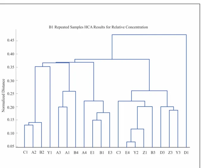
Figure 4.9 B1 Repeated Samples HCA Results for the Relative Concentrations ...54
Figure 4.10 B2 Glacier Conceptual Sampling Map ...55
Figure 4.11 B2 End-Members' HCA Results for Absolute Concentration, 07/07/2015 ...56
Figure 4.12 B2 End-Members' HCA Results for Relative Concentration, 07/07/2015 ...57
Figure 4.13 B3 Glacier Conceptual Sampling Map ...58
Figure 4.14 B3 End-Members' HCA Results for Absolute Concentration, 07/07/2015 ...59
Figure 4.15 B3 End-Members' HCA Results for Relative Concentration, 07/07/2015 ...60
Figure 4.16 Stable Heavy Water Isotope Variations of the 24-hour Sampling ... 61
Figure 4.17 Ionic Variations over the 24-Hour Sampling ... 62
Figure 4.18 Precipitation Height Recorded during the 24-hour Sampling ... 63
Figure 4.19 HBCM Results for B1 Glacier on 03/07/2015 ... 65
Figure 4.20 HBCM Results of B1 Glacier on 05/07/2015 ... 67
Figure 4.21 HBCM Results for the B Watershed on 07/07/2015 ... 69
Figure 4.22 Glacial vs Non-Glacial and Precipitation Relative Volumes over 24-hour Sampling Cycle ... 72
LIST OF ABREVIATIONS
AWS Automatic Weather Station
Ca2+ Calcium ion
CaCO3 Calcite
Cl- Chloride ion
DOC Dissolved Organic Carbon EMMA End-Member Mixing Analysis eq Equation
F- Fluoride ion
GW Groundwater H2SO4 Sulphuric Acid
HDPE High Density Polyethylene HCA Hierarchical Cluster Analysis
HBCM Hydrochemical Basin Characterization Method
HNO3 Nitric Acid
IC Ionic Chromatography
ICP-OES Inductively Coupled Plasma Optical Emission Spectrometry
K+ Potassium ion
KNPR Kluane National Park and Reserve Ksp Solubility Product Constant
Na+ Sodium ion
Mg2+ Magnesium ion
Q Ion Activation Product
SO42- Sulfate ion
SWE Snow Water Equivalent
TDS Total Dissolved Solids V-SMOW Vienna Mean Ocean Water
LIST OF SYMBOLS AND UNITS OF MEASUREMENTS mg/L Milligram per liter, concentration unit
µS/cm Microsiemens per centimeter, electrical conductivity unit mL Milliliter, volume unit
mmol·L-1 Milli-moles per liter, concentration unit
m·y-1 w.e. Meters per year water equivalent
N Normality
INTRODUCTION
Climate change is affecting regions in the world in different ways varying on the area and their respective environments; it has led to major changes in the annual hydrological cycle of arctic and subarctic territories, affecting the livelihoods and well-being of their respective ecosystems (Deb, Butcher et Srinivasan, 2015). In these regions, the effect of increasing temperatures is particularly pronounced due to the presence of climate sensitive features such as snowpack, glaciers and permafrost. Some of the visible hydrological changes in response to climate warming have been earlier spring melt periods (Manabe et al., 2004; Nijssen et al., 2001); glacier recession and related hydrological responses (Kaser et al., 2006); shorter periods of snow cover and related shift in peak flow timing (Brown et Braaten, 1998; Whitfield, 2001) and permafrost thawing that could result in an increased runoff (Walvoord et Striegl, 2007).
Hydrological changes in northern regions have numerous consequences for both populations and ecosystems. Hydrological changes have already resulted in marked regime shifts in the biological communities of many lakes and ponds (Schindler et Smol, 2006). Partly due to increased water temperatures, fish populations, like Salmonid species, have considerably decreased over the last centuries (Grah et Beaulieu, 2013). Changes in flood regimes associated to snow cover alteration will affect ecosystems and sediment transports (Lotsari et al., 2010). Changes in river ice regimes affect access to resources and population movements (Wilson, Walter et Waterhouse, 2015). Other effects of hydrological changes include increased risks to infrastructures and water resources planning as well as a rise in nutrients and carbon outflows to the ocean (Bring et al., 2016).
The St. Elias Mountains, situated in the Canadian and American subarctic, are the headwaters of the Yukon River Basin and therefore plays a huge role in the hydrology of its watershed. Because these mountains host the largest icefields outside of the polar icecaps, the St. Elias Mountains’ hydrology is highly influenced by glaciers (Fleming et Clarke, 2003). Thinning rates in the Yukon glaciers alone are estimated between 0.45 ± 0.15 m·y-1 water equivalents
(w.e.) and 0.78 ± 0.34 m·y-1 w.e (Barrand et Sharp, 2010; Flowers, Copland et Schoof, 2014)
resulting in ubiquitous mass loss of 22% glacier loss in the last 50 years (Barrand et Sharp, 2010). Rapid mass loss from the glaciers of this range was shown having a direct measurable impact on the global sea levels (Flowers, Copland et Schoof, 2014). The long term influence of glaciers’ retreat on hydrological regimes is known as the Peak water (Baraer et al., 2012): glaciers produce an initial increase in runoff as they lose mass. The discharge then reaches a plateau called “peak water" and subsequently declines as the volume of glacial ice continues to decrease. Other known impacts of glacier retreat on hydrology are changes in diurnal oscillation of stream discharge (Singh et al., 2005), timing of the maximum and minimum annual discharge (Janowicz, 2011), water temperature (Blaen et al., 2014) and sediment transport (Lotsari et al., 2010).
However, glaciers are not the only water source in subarctic glacierized catchments. Groundwater, whose contribution is highly related to permafrost conditions in those environments (Janowicz, 2011), plays a huge role in subarctic glacierized catchments’ hydrology (Levy et al., 2015; Walvoord et Striegl, 2007). Other water sources such as buried ice bodies (Schomacker et Kjær, 2008), ice-cored moraines (Moorman, 2005) or icing (Moorman et Michel, 2000), even if by far less studied, also make potential water sources in such environments.
Facing challenges of climate change adaptation in this region of the world will require informing policy makers on how to manage water security (Bring, Jarsjö et Destouni, 2015) and therefore anticipating evolution of the different water sources that make river discharges. Thus, few studies have considered the role of extra-glacial water sources in glaciers fed catchment hydrology (Milner, Brown et Hannah, 2009). As stated by Rouse et al. (1997) ”There is a clear need to improve our current knowledge of temperature and precipitation patterns…to understand better the interrelationships of cold region rivers with their basins”. In this context, glaciers hydrological role has captured most of the scientific attention over the last decades, while hydrological processes of proglacial areas remain under studied (Heckmann, McColl et Morche, 2016).
The overall objective of the present study is to improve the understanding of hydrological processes in proglacial areas of glacierized headwater catchments in the St. Elias range by identifying sources and quantifying their contribution to the runoff of a small watershed (named B Valley) of the Duke River watershed in the Kluane National Park and Reserve (KNPR) during summer 2015. This overall objective can be divided into three sub-objectives:
1. Identification of the main water sources by the mean of their physico-chemical particularities at different dates of the study period.
2. Estimation of the said sources’ contribution to total discharge by using a mixing model again at different dates of the study period.
3. Differentiation between glacial and non-glacial contributions to the outflows of the B Valley during a 24-hour period.
To meet these objectives, a synoptic series of sampling conducted in the B Valley between July 3rd and 10th 2015 were undertaken. Samples were then analyzed for major ions, organic
carbon and heavy stable water isotopes, which were used as natural tracers to identify water sources and estimate their contribution to outflows. Quantification of sources’ contribution was achieved using the hydrochemical basin characterization method (HBCM), a method developed to answer such question in the context of tropical glacierized watersheds (Baraer et al., 2015).
This chapter will present the knowledge already accumulated on the characterization of hydrological processes using natural tracers. Starting with a general introduction of the studied environment and its hydrological processes; the concerned sources will then be dissected and tracers previously used to differentiate them will be revealed. Finally, a broad introduction to mixing models will be narrowed down to the hydrochemical basin characterization method (HBCM), the model used in this study.
1.1 Subarctic Area
Subarctic environments are the regions in the northern hemisphere south of the Arctic generally falling between 50ºN and 70ºN parallels. With increased temperatures, subarctic hydrological sources will be affected and in turn will affect runoff volumes, a temporary increase in volumes is anticipated, which will increase erosion and habitat loss to local wildlife (Nuttall, 2007). This study focuses on the environmental changes due to global warming in the subarctic region of Canada and more precisely the St. Elias Mountain Range area.
1.1.1 St. Elias Mountain Range
The St. Elias Mountains are a segment of the Pacific Coast Ranges in northwestern North America. They are situated on the Canadian/Alaskan border, each building a protected area surrounding it: the Wrangell-St. Elias National Park and Preserve in the USA and the Kluane National Park and Reserve in Canada as seen in figure 1.1. With close to 46 000 km2 of ice cover (Berthier et al., 2010), the St. Elias Mountains host the largest icefields
outside the polar icecaps.
CHAPITRE 1 LITERATURE REVIEW
Figure 1.1 St. Elias Mountain Range, Study Site Location Modified from Ricketts (1999)
The St-Elias mountain range is the headwater of the Yukon River Basin. The Yukon River empties out into the Bering Sea at the Yukon-Kuskokwim Delta as pictured in Figure 1.2. The Yukon River Basin is the fourth largest watershed in North America (831 390 km2), its runoff occurring mainly during summer months from snowmelt, rainfall and glacial melt (Hay et McCabe, 2010).
Figure 1.2 Yukon River Basin Taken from Brabets et Schuster (2008)
The high rate of mass loss of glaciers in the St. Elias region shows significant contribution to global sea level rise (Arendt et al., 2002; Luthcke et al., 2008). An increasing number of studies are conducted in an effort to understand the response and corresponding impact these rapid changes will have (Berthier et al., 2010; Deb, Butcher et Srinivasan, 2015; Flowers, Copland et Schoof, 2014; Johnson, 1992).
Anticipated hydrological changes in this region of North America are predicted to particularly affect aboriginal populations. For instance, aboriginal peoples located along the Yukon River in both the United States and Canada depend on fish populations for livelihood (Nuttall, 2007), local people have described the environment as of risk and at risk, meaning that climate variability has changed movement and behavior of animals making everyday traditions and activities unpredictable, and at risk because of pollution, industrial development and global warming induced changes (Ørbæk et al., 2007).
1.1.2 The Duke River Valley
The present study takes place in the upper part of the Duke River valley. The Duke River empties into the Kluane River just below Burwash Landing, which in turn feeds the White River and consequently spills into the Yukon River in the watershed holding the same name. The study site is a small watershed (631 km2) found in the southeast part of the range home to the Duke River (Figure 1.3 - red outline), the glacier feeding the river holding the same name is 20.1 km2 (see Chapter 2 - Study Site).
Figure 1.3 Duke Upper Watershed
1.2 Water Sources in Subarctic Glacierized Watersheds
As discussed in the introduction chapter, glacierized watersheds of the subarctic host a large number of potential water sources. Glaciers, the most studied water source, play a dominant role in the watershed they belong to (Kang et al., 2009). However, other water sources, most of them being climate sensitive, shall also be considered as potential important contributors to glacierized watershed outflows. Figure 1.4 shows, in a conceptual way, the different features that play a role in the subglacial environment. In addition to the glacier related
processes, groundwater (Walvoord et Striegl, 2007) is highly dependent on the permafrost conditions (Janowicz, 2011) in those environments, ice cored moraines (Moorman, 2005) or icing (Moorman et Michel, 2000) and rock glaciers appear to also be important factors.
Main hydrological characteristics of glacierized watersheds and proglacial fields are glaciers, ice-cored moraines, rock-glaciers, permafrost and snow cover as presented in figure 1.4. These features are affected by the energy balance with radiation as the largest flux input, hydraulic processes acting within and hydrological effects acting on them.
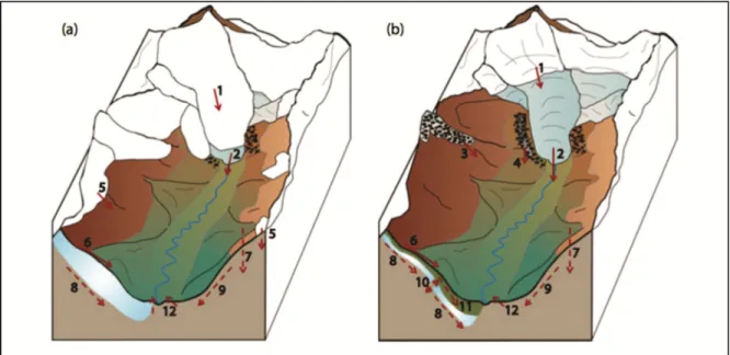
Figure 1.4 Conceptual model of the subarctic glacierized watershed for two seasons: (a)snowmelt and (b) summer; red arrows show water fluxes (solid - above the ground, dashed
- under the ground): 1 - snowmelt on the glacier, 2 - glacier melt, 3 - ice melt from rock glacier, 4 - ice melt from ice-cored moraine, 5 - snowmelt of the glacier, 6 – surface runoff, 7
– precipitation infiltration, 8 – sub-permafrost groundwater, 9 – groundwater, 10 – intra-permafrost groundwater, 11 – supra-intra-permafrost groundwater, 12 – springs
Taken from Chesnokova (2015)
Runoff from the glacier is composed of snowmelt on the glacier (1) and glacier melt (2). Gradually, the snowmelt will occur at higher elevation as summer progresses leaving the glacier uncovered and therefore melting at a faster rate. When snow melts on the edges of the glacier, ice-cored moraines (4) and buried-ice (3) are also exposed to melt during summer
season; due to their insulating debris cover, buried ice melt volumes are dependent on size and energy inputs. As snow melts, it creates a surface runoff (6) that progressively infiltrates the soil and finds its way into the hydrological processes within permafrost. Surface runoff and precipitation (7) are the major hydrological actors in seasonal growth of the permafrost active layer, they supply supra-permafrost groundwater sources (11) but will also contribute to hydraulic processes acting upon sub- (8) and intra-permafrost (10) groundwater. Due to North-facing slopes receiving less solar radiation, they usually have more permafrost (Carey et Woo, 1998; 2001) and higher snow water equivalent (SWE) prior to melt. Groundwater is also commonly found lower in the valley where it may find soils to infiltrate or in phases of permafrost to permeate through.
In this study site, only glaciers, icings, ice-cored moraines and groundwater sources were present. In the following section, we describe the main sources expected in this subarctic watershed in more details.
1.2.1 Glaciers
Glaciers present a substantial freshwater source which globally supply water to one sixth of the world’s population (Barnett, Adam et Lettenmaier, 2005). Despite growing concerns for the health of glaciers and their implications in water supplies (Cruz R. V. et al., 2007), their global contribution is not yet well understood (Schaner et al., 2012). Glaciers store water in the solid form in the accumulation area during accumulation months and release most of their contribution during the ablation season.
Glaciers are complex entities, although their contribution is confined to meltwater for the ablation zone, there are multiple pathways it can follow; surface (supraglacial), internal (englacial), and basal (subglacial) all contribute to runoff composition (Boon, Flowers et Munro, 2009). The role and activity of those pathways in the hydrological systems are variable in time and space (Irvine-Fynn et al., 2011) and can be difficult to isolate.
Runoff volumes from glaciers follow the diurnal cycle. They are affected by melting season variability as well as accumulation volumes, consequently making accurate response projections difficult. Their runoff volumes are controlled by i) melt water production at the glacier-atmosphere interface, ii) volume of water it stored during the accumulation period and iii) the pathways melt water employ within the glacier surface whether it is supra-, en- or subglacial (Chesnokova, 2015). Supraglacial melt is the dominant source of meltwater for most glacierized area (Hock, 2005), as most of the melt occurs at the glacier surface. On the surface of the glacier, supraglacial channels are eroded onto the surface and meltwater finds its way into the englacial and subglacial systems via crevasses and moulins. Either through ice percolation (slow system) or englacial channels (fast system) the water will drain into the glacier’s hydrological pathways (Benn et Evans, 1998). With increasing volumes during the ablation season, the pressure created within the glacier will lead to wider channels, faster snowline retreat and enhanced hydrofracturing, hence the ever changing drainage system course during melting season.
Daily, meltwater reaches its peak volume shortly after the shortwave radiation and temperature maxima (Chesnokova, 2015). Seasonally, the annual runoff reaches its peak during the ablation season, when average radiation and temperature are at their peak.
There are multiple types of glaciers based on location, form and temperature regimes. Glaciers from the Northern St. Elias slopes are classified as mainly polythermal (Benn et Evans, 1998). Polythermal glaciers are defined as “ice masses displaying a perennial concurrence of temperate (temperature at melting point) and cold ice (temperature below melting point)” (Irvine-Fynn et al., 2011). Their particular thermal regime makes the supraglacial pathway dominant compared to englacial and subglacial channels, this being at least true in the cold ice section of the glacier.
1.2.2 Ice-Cored Moraines
Moraines are glacially accumulated piles made up of glacial debris, which range from small flour-like soil to large boulders (Menzies, 2002). There are two main types of moraines: lateral moraines form at the edges of the glacier pushed by ice flow over time, and terminal moraines, as their name suggests, are at the foot of the glacier marking the maximum advance of the glacier (Barr et Lovell, 2014).
Ice-cored moraines are ice bodies that comprise a discrete body of glacier ice covered with morainic materials (Singh, Singh et Haritashya, 2011). The formation of moraines is based on a combination of supra-, en-, and subglacial debris being pushed to the edges. Proglacial debris are forced outward during glacier advance, subglacial debris can be squeezed from upward pressure as well as surrounding ridges contributing to the amount of sediment (Lukas et al., 2005).
For an ice-cored moraine to emerge, ice must be isolated from the glacier during advances but covered by enough debris to shield it from melting, thus creating a differential ablation rate than that of the glacier’s (Lukas, 2011). Lukas (2011) proposed three buried-ice formations; active ice near the glacier’s boundaries covered in sediment and debris are cut-off during negative mass balance, steady delivery of debris at the same location (depocenters) can lead to thickened supraglacial material cover changing the ablation rate, and finally existing dead ice can be engulfed by advancing glaciers. The debris cover affects the thermal conductivity and therefore the insulation provided by the debris above and below the ice affects the melting rate and by consequence the volume of water contributed. The thicker the debris cover, the slower the ablation rate (Brook et Paine, 2012), exposing bare ice can increase ablation rate up to 30 cm in a 1.5 month period (Johnson, 1992).
1.2.3 Rock Glaciers
Rock glaciers, behave differently than glaciers, because they consist of an ice-core covered in debris or an ice-cemented matrix (Singh, Singh et Haritashya, 2011). The insulating properties of the debris cover (Humlum, 1997) reduce and can even eliminate the characteristic glacier dynamics. Thus, rock glaciers contribute water to total discharge by snowmelt and precipitation infiltration, permafrost melt and ice-core melt (Williams et al., 2006) and can stay frozen even with the absence of snowpack cover. The interior of a rock glacier can act as an aquifer and the hydrological characteristics of the rock glacier can be viewed as its own system (Singh, Singh et Haritashya, 2011).
1.2.4 Groundwater
Groundwater is a very broad term to describe water that occupies empty spaces in soils and geographic strata (Groundwater, 2016). It englobes a mixture of sources and as it sits underground in soil layers, it absorbs its organic properties.
Groundwater drawn from periglacial sources, such as moraines and rock glaciers have been shown to affect the timing and volume of alpine discharge (Langston, Hayashi et Roy, 2013). In high latitude soils that reach temperatures below freezing point (0°C), permafrost can also contribute to groundwater source volume; glacial drainage can also promote the formation of permafrost or buried ice features (Irvine-Fynn et al., 2011). The active layer is defined as the stratum that melts and refreezes with temperature changes (Osterkamp et Burn, 2003). As active layers are becoming thicker due to climate change, water faults are growing and water melting through these faults reaching groundwater networks only contributes to the growth of the layer (Osterkamp et Burn, 2003; Shur et Jorgenson, 2007). Permafrost zones are affected by multiple local factors such as topographic location, slope, vegetative cover, snow cover and soil texture. The permafrost cover in the St. Elias range is measured to be sporadic discontinuous, meaning permafrost can be found in 10-50% of the soil, with temperatures close to 0ºC (Burn, 1994). Multiple researches have been conducted on permafrost in the
Kluane lake region since the 80s, notably on the topic of active layer evolution (Harris, 1987) and permafrost probability modelling (Bonnaventure et Lewkowicz, 2008; Kinnard et Lewkowicz, 2005), but little is known on its possible contribution to total runoff. Groundwater has been found to be an important recharge source and possibly a potential buffer on the impact of predicted lower glacial discharge (Baraer et al., 2012; Langston, Hayashi et Roy, 2013).
1.2.5 Icing
Icings are the results of refreezing at the surface of emergent discharge from sub-surface sources such as groundwater sources (Hodgkins, Tranter et Dowdeswell, 2004; Williams et Smith., 1989). They are commonly found in the proglacial field, but not limited to permafrost regions. They can also be fed by subglacial meltwater during accumulation season and go through annual cycle of growth and decay. Glacier fed icings have a fragile dependence on glacier and can easily be overthrown by change in hydrological conditions (Wainstein, Moorman et Whitehead, 2014). Their contribution to overall discharge is dependent on their size and melting rates.
1.3 End-Members’ Contribution to Catchment Outflows
There are multiple techniques to quantify relative contributions of end-members: Direct discharge measurements, glaciological approaches, hydrological balance equations, hydrological modelling and finally use of hydrochemical tracers. Direct discharge measures are done at end-member’s outlets, which can be difficult and hard to access given the changing landscape in glacial environments (Gascoin et al., 2011; Thayyen et Gergan, 2010). Glaciological approaches are based on the estimate of glacial mass changes (Liu et al., 2009); they are potentially the most accurate method but are limited to one end member only and existing datasets (La Frenierre et Mark, 2014). The hydrological balance equation method deduces glacier meltwater discharge (Baraer et al., 2012) where other component contribution can be estimated and using hydrological modelling, as the name suggests, relies
on models specific to watersheds (Comeau et al., 2009), but again both depend heavily on the common understanding of involved processes. Hydrochemical tracers based methods solve the hydrological balance equation by assuming conservative behaviour of the tracers (Baraer et al., 2009). Geochemical techniques and end-member mixing models have been used increasingly to characterize contributions in watershed under varying environmental conditions (Baraer et al., 2015; La Frenierre et Mark, 2014). Based on its chemistry, it is possible to “quantify the proportion” of end-members to discharge (La Frenierre et Mark, 2014). This method will be explained further in more detail.
1.3.1 Natural Tracers
Water from different end-members tends to have a distinct hydrochemical signature; its unique path is subject to specific geological, and hydrochemical processes (Drever, 1988). The individual end-member signature is then used for understanding the hydrological, geological and biological processes an end-member may be subject to and to quantify their contribution to total runoff discharge (Baraer et al., 2015).
Commonly used natural tracers dab in both chemical and physical properties. Chemically, ionic concentrations are the most prevalent source of information; anions frequently used are SO42-, Cl-, F-, HCO3-, NO3- and cations used are Na+, K+, Mg2+ and Ca2+ (Lafreniere et Sharp,
2005; Mitchell et Brown, 2007). Organic contents have also recently emerged as efficient tracers for groundwater and permafrost sources (MacLean et al., 1999). Known signatures include organic nitrogen and carbon concentrations. In this study, organic carbon was utilized in efforts to identify permafrost contributions. Physical properties of water sources include isotopic ratios and electrical conductivity. Isotopes frequently used are the heavy stable water isotopes 18O and 2H, which were used in this study but other isotopes are sporadically used
depending on environment and specific features.
Usually, natural tracers based methods imply the use of different kind of tracers in order to benefit from their different characteristics. For instance, major ions are most effective in the
differentiation of groundwater sources from other end-members while stable isotopes are more efficient in the distinction between glacial meltwater from precipitation and snowmelt, so they are usually used in combinations with one another (Baraer et al., 2012; Mark et Seltzer, 2003).
1.3.1.1 Major Ions
Solute tracers are very convenient because they tend to be specific to an origin affected by its own environmental, biological and geological pressures (La Frenierre et Mark, 2014) and so sources will have a unique ionic signature based on their origins. The various components of the hydrological cycle are dominated by different solutes, for example, precipitation would contain higher concentrations of chloride (Cl-) because of its presence in oceanic water and the evaporation cycle (Ladouche et al., 2001). Mg2+ and Ca2+ ions on the other hand are usually a by-product of bedrock geology and chemical weathering (Bagard et al., 2011; Brown et al., 2006; Tranter et al., 1996). The use of solutes as tracers is only limited by the reactivity of the tracers, whether it is in its natural state, the transportation process, or in the analytical procedure.
The ions recognized as majors are NO3-, SO42-, F-, Cl-, HCO3-, Na+, K+, Mg2+ and Ca2+ (Baraer et al., 2009; Brown et al., 2006; Mitchell et Brown, 2007). Other ionic compounds such as
Br-, Al-, Fe2+,3+, Mn2+,3+,4+, PO43- and NO3- (Barthold et al., 2010; Crompton et al., 2015) have already been used as tracers in several studies but their use is limited by their chemical instability in natural conditions. Silicate is also a stable solute for reconstruction of hydrological pathways; it has been used in ratio with other solutes as a tracer for multiple end-members (Klaus, 2013; Laudon et Laudon, 1997).
Solutes have proven particularly efficient in subarctic environments. For example, studies show that icings layers can be used as a solute record of highly concentrated early spring runoff, which is released in the early ablation stages (Wadham, Tranter et Dowdeswell, 2000). Yde et al. (2012) show high concentrations of Ca2+ and HCO3- as well as cryogenic
calcite (CaCO3) precipitate especially at the extremities, while isotopic data shows a normal trend with the local meteoric water line. Ionic concentrations are powerful tracers best used in unison with isotopic ratios.
1.3.1.2 Isotopes
The most used isotopes for hydrological sciences are the δ18O for oxygen and δ2H for hydrogen; they hold the same position in the table of elements as their most abundant counterparts, 16O and 1H respectively (Gat, 2010). They are referred to as the heavy stable water isotopes.
Other isotopes such as the radioactive tritium 3H (Maloszewski et al., 2002; Turnadge et Smerdon, 2014) and 222Rn (Dugan et al., 2012; Elliot, 2014), as well as stable strontium isotopes 86Sr and 87Sr (Bagard et al., 2011; Keller, Blum et Kling, 2010) and sulfur isotope 34S (Elliot, 2014) have been used in different studies as tracers for permafrost and groundwater end-members and even moraine tracing (Stotler, Frape et Labelle, 2014). However sampling and analyses for those isotopes are impractical in standard conditions: 3H
has to be collected in glass bottles (100 mL), 222Rn is highly volatile gas (Freyer et al., 1997),
strontium and sulfur isotopic ratios are determined by costly and labour intensive methods (Martins et al., 2008; Mason, Kaspers. et van Bergen, 1999). For a large number of samples, stable heavy isotopes of water are the most practical and cost effective analytical method.
Measurements leading to a more intuitive measure are expressed as ratios relative to the Vienna Standard Mean Ocean Water (V-SMOW) as shown in eq 1.1 and 1.2. R is the isotopic ratio, expressed in permil, calculated as a ratio of concentration between the rare and abundant isotope.
18R = = // (1.1)
δ O = x 1000 = − 1 x 1000 (1.2)
By definition, the standard mean has a composition of 0‰ for both heavy isotopes, representative of the average sea concentration. It is also well known that ratios change based on altitude, being increasingly depleted at higher elevation (Gat, 2010) due to the progressive condensation and precipitation processes in high mountainous areas (Gonfiantini et al., 2001). Due to their heavier weight and larger mass (Gat, 2010), they can induce measurable physical and chemical effects; during phase changes in the hydrological cycle, heavy isotopes will become enriched in one phase and depleted in the other, this separation is known as isotopic fractionation (Gat, 2010). For example, in warm temperatures, evaporation will occur and the phase change of a lighter molecule requires less energy, hence the gas phase would contain H O while the liquid phase would be left with the heavier molecules being enriched in H O.
Because isotopes are affected by evaporation and transpiration, they can induce a specific signature in recharge water, which will be significantly different from isotopic ratios in precipitation samples (Hopmans, 2000; Stumpp et al., 2009).
1.3.1.3 Dissolved Organic Carbon
Dissolved organic carbon (DOC), is a good indicator of biological processes. DOC is defined as organic matter that passes through a filter, usually 0.22-0.7 µm (Brukner, 2016). As a tracer, DOC is usually used for permafrost or groundwater end-member tracing (MacLean et al., 1999), because of extended exposure to organic soil leaching, permafrost has been associated with high organic content (Carey et Quinton, 2005; Kokelj, Smith et Burn, 2002). Permafrost-dominated catchments showed higher concentrations of DOC, but lower solute contents than their neighbouring nearly permafrost-free watersheds (Carey et Pomeroy, 2009). DOC has been used with δ18O, (Carey et Quinton, 2005), and with HNO3- (Petrone et al., 2006) as tracers in important organic layer environments.
1.4 Mixing Models
The unique hydrochemical signatures of end-members are the basis of hydrochemical mixing models. By using conservative tracers, it is possible to identify sources and quantify their contribution to runoff (Baraer et al., 2009; Christophersen et Hooper, 1992; Mark, McKenzie et Gomez, 2005). The simplest mixing models are two end-member models, (e.g. glacial and non-glacial) (Mark, McKenzie et Gomez, 2005). Models distinguishing more end-members (glacier melt, surface runoff, groundwater discharge) require the use of statistical methods (e.g. Bayesian) (Baraer et al., 2009; Cable, Ogle et Williams, 2011).
There are two techniques dominating hydrological tracer studies: hydrograph separation and end-member mixing analysis (EMMA) (Barthold et al., 2011). The first relies on solving mass balance sets of equations while the latter is based on the eigenvalues approach. The use of a mixing model is to identify and quantify the major contributors of total discharge. EMMA is unrestrictive in the amounts of tracers needed (Barthold et al., 2011); two to six seems to be the majority, but the more end-members the more tracers are required. Its restrictive factor is the repetitive sampling required, which can be problematic in remote locations and difficult to access terrain (Christophersen et Hooper, 1992; Sinclair, 2014).
For the hydrochemical tracer technique to be employed there are key assumptions to take into account. Firstly, the hydrochemical signature associated to each end-member must be sufficiently distinct. Followed by the notion of conservation of the tracer between the sources and mixing points, meaning there are no further changes occurring, such as isotopic fractionation or chemical reaction which would affect solute concentrations (Baraer et al., 2009; Mark, McKenzie et Gomez, 2005). This ensures that the mass of the solutes found in the mix describes an accurate portrait of the relative inputs of the end-members involved (Baraer et al., 2009; Christophersen et Hooper, 1992). The hydrochemical tracer approach also assumes the chemical characteristics defining end-members take into account the range of hydrochemical variation each source might experience (La Frenierre et Mark, 2014) in a way, minimizing the variability of end-members. For instance, glacial meltwater would combine a mixture of different ablation processes and varying flows that would be conditioned to varying isotopic fractionation and chemical reactions (Nolin et al., 2010; Sharp et al., 1995). Glacial derived meltwater in a single watershed can originate from multiple chemically-distinct glaciers that have their own unique bedrock geology, ice flow rates and subglacial drainage patterns (Yuanqing et al., 2001).
These assumptions limit the hydrochemical tracer approach, but there are notable advantages over certain techniques. For example, chemical tracer analysis does not require long term detailed meteorological and glaciological data; a sampling period is usually sufficient to establish a logical snapshot of base flow conditions and pathways. La Frenierre et Mark (2014) also argues that the hydrochemical tracers approach doesn’t require explicit calculation of hydrological parameters that can be challenging to accurately measure in the field such as evapotranspiration and groundwater exchange (Kong et Pang, 2012; Mark, McKenzie et Gomez, 2005). Hydrochemical data is rather easy and inexpensive to obtain despite a watershed’s seclusion (Mark et Seltzer, 2003; Nolin et al., 2010).
The hydrochemical basin characterization method (HBCM) used in the present study, is one of the methods used to assess end-members’ contribution to outflows at various points of a watershed. Based on hydrograph separation techniques, HBCM was developed to
characterise contribution of end-members in remote glacierized watersheds, where EMMA cannot be adopted due to logistical reasons.
HBCM has been used previously for quantifying groundwater contributions in the tropical glaciers of the Cordillera Blanca in Peru, more precisely the Callejon de Huaylas watershed (Baraer et al., 2009; Baraer et al., 2012). It was successful in producing reliable results in ungauged and remote areas (Baraer et al., 2009). It has also showed positive results in two sites of the Central Andes, the Tuni watershed in the Cordillera Real in Bolivia and the Pastoruri watershed in the Cordillera Blanca in Peru (Sinclair, 2014).
HBCM requires samples to be collected in a limited time-frame, following a synoptic approach, in order to generate a geospatial snapshot of the hydrological systems inner-workings within a watershed. Some of the downfalls of this method are that it is difficult to be certain, with high confidence, that the assumptions previously mentioned, which are the core components of the method, are being met. In a dynamic, geologically heterogeneous, mountain watershed, it proves to be challenging to verify the conservation of a tracer and the true unique hydrochemical signature of an end-member, even more so when only a small number of samples are collected (Nolin et al., 2010). Despite those limits, trace methods based techniques have proven very efficient for hydrograph separation in alpine environments (Baraer et al., 2009; Baraer et al., 2015; Fujita, Ohta et Ageta, 2007; Mark et Seltzer, 2003).
Although the technique has proven itself, it has yet to be tested in subarctic glacierized catchments.
The Duke valley is located in the St. Elias mountain range in the Yukon; it has a total area of 631 km2 and its elevation ranges from 817 to 2824m. The valley was chosen partly due to its
location and relative accessibility, but also because a gauging station situated at the lower part of the Duke River, near the mouth where it intersects the Alaska Highway (61° 20ʹ 45ʺ N, 139° 10ʹ 04ʺ W) monitors stream discharge since 1981. The Duke River watershed provides an ideal sized watershed for field work periods and distances.
As of 2015, the upper Duke River watershed is being equipped with hydro-meteorological equipment with the objective of studying hydrological impacts of climate change in the St. Elias Mountains. The research program, led by École de Technologie Supérieure (ETS), aims to improve the understanding of unique hydrological processes by focusing on glacier fed watersheds at the regional scale and their specific features scale. The uppermost part of the watershed, where most of the research activities took place was subdivided into smaller watersheds; the main study area, watershed B, is highlighted in green in the previously presented figure 1.3. We used the watershed B to evaluate and provide a primary understanding of the hydrological processes of this alpine environment.
The watershed B was chosen for both scientific (i.e. the presence of multiple glaciers and an important proglacial field) and logistical reasons (i.e. its relatively small size and accessibility). Valley B hosts three small glaciers we named B1, B2 and B3 (Figure 2.1). In total, the watershed B has a surface of 8.75 km2 and is 36.6% glacierized.
B1 is the largest of those glaciers with 1.7 km2 area and the one with the lowest terminus
(Table 2.1). B2 is second in size with an area of 0.9 km2 and altitude terminus elevation of
2129 m, B3 is the smallest and highest glacier in the watershed with 0.6 km2 of glacierized
area and a terminus at 2272 m.
CHAPITRE 2
A survey was conducted by the Yukon Geological Survey in 1992 to identify bedrock geology and lithology in the Kluane National Park and Reserve. The B valley is composed of two regional terranes with slight variation in bedrock composition. The higher in altitude covers most of the icefields area. It is made of principally sedimentary rocks containing mainly siltstone, sandstone, quartzite and schist and in minor quantities argillite, phyllite, limestone, volcanic, gypsum and anhydrite (Dodds et Campbell, 1992). The lower altitude bedrock content is a mixed of volcanic and sedimentary rock, the principal lithology includes sandstone, conglomerate, breccia, greenstone and amphibolite while minor lithologies includes argillite and phyllite (Dodds et Campbell, 1992).
Table 2.1 Glaciers of the B Watershed Name Total Glacierized
Area Altitude of the terminus B1 1.7 km2 2038 m B2 0.9 km2 2129 m B3 0.6 km2 2272 m
During the field campaign of 2015, many unexpected hydrological features and water sources were observed such as icings, buried ice and ice-cored moraines scattered throughout proglacial fields. Slopes neighboring glaciers were producing small streams, possibly due to buried ice. Groundwater wells were dug in various areas of the watershed, but no permafrost was found, partially due to geological features, wells could not be built deeper than 1.5 m.
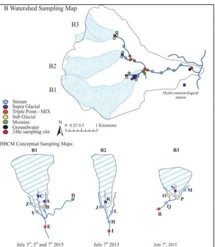
As seen in figure 2.2, 67 samples were collected in total for the sampling of the B watershed. At sampling locations, site measurements were taken such as pH, electrical conductivity, and temperature (appendix I). Sampling for ionic content, organic carbon concentration, isotopic ratios and alkalinity testing were conducted. B1 glacier was sampled on four occasions during the sampling period, twice on July 3rd, and once 5th and 7th 2015. The July 3rd sampling was exceptional due to a snow precipitation on July 2nd. Therefore, the B1 system was studied in two parts, first a spatial analysis with the established system on July 5th and secondly a temporal analysis was done on the entirety of the sampling. B2 and B3 glaciers were sampled once during the sampling period in one day, July 7th, 2015.
The B outlet was also sampled over a 27-hour period at 2-hour interval from 9h to 21h and at a 4-hour interval from 21h to 9h, for a total of 10 samples, from 09/07/2015 at 5h09 to 10/07/2015 at 8h15. This was done to capture the fast changes during the day while we expected the night variations to be much smaller.
Figure 2.2 B Watershed Sampling Map
In addition to sampling, over the course of the campaign, long term hydro-meteorological equipment was installed at the outlet of the B valley, pressure gauge stations were placed in strategic outlets to measure water discharge and time-lapse cameras were placed to visually assess the evolution of subarctic proglacial field. The hydro-meteorological equipment set on an automatic weather station (AWS) (60°59'44.0"N, 138°57'45.4"W) recording air temperature, liquid precipitation, radiation and relative humidity at 15 minute intervals. This dataset provides information on the micro-climate of the valley and will eventually be used in a numerical model (Chesnokova, 2015). Stream gauging stations equipped with pressure transducers were installed in the B valley outlet and the Duke River outlet.
On the field, all collected samples had site measurements taken as outlined in the previous chapter, those were then analysed for isotopic ratios, DOC and major’s ions following the outlined methodology. Raw data was manipulated to produce a set of calculated tracers such as relative concentrations and total dissolved solids (TDS). A bivariate analysis was then conducted on the measured and calculated tracer concentrations in order to identify tracer signatures unique to end-members. This was then followed with a hierarchical cluster analysis (HCA) to identify end-members’ origins and pathways employed. Using HCA also offered the opportunity to establish any relationship with groundwater sources. HCA results were utilized to select tracers needed for the quantitative analysis in the hydrochemical model. A quantitative study was done using the hydrochemical basin characterization method (HBCM) for the B watershed and for the 24-hour sampling period. The following sections will go into greater depth and detail into the methods used for each component of this study.
3.1 Sample Collection and on Site Measurements
On site, the GPS coordinates were measured using a Magellan™ Triton® 300 while pH, conductivity (µS/cm) and temperature (ºC) were measured using a PCE-PHD-1 pH meter.
Samples for stable isotope analysis were collected in 30 mL high density polyethylene (HDPE) bottles. The bottles were rinsed three times with water at the source, and then filled to the brim with the sample. The bottles were then sealed with insulating tape to avoid evaporation.
Samples for dissolved organic carbon (DOC) and major ion samples analysis were filtered with hydrophilic polypropylene 30mm syringe filters (0.45 µm) with 50 mL syringes. HDPE
CHAPITRE 3 METHODOLOGY
60 mL bottles were rinsed three times with filtered water, filled to the brim and sealed with insulating tape. Bottles were stored in the dark at 4°C whenever possible.
Samples for alkalinity analysis were collected in 125 mL HDPE bottles that were rinsed three times with unfiltered water and then filled to the brim with unfiltered source water.
3.2 Chemical Analyses
3.2.1 Laboratory Analyses and Tracer Value Calculation
Alkalinity was tested within 12 hours of sampling at the base camp. Tests were conducted by titration with 0.1600N H2SO4 with a HACH® Digital Titrator 16900, using bromocresol green as an indicator. An aliquot was first used to thrice rinse all the equipment, and then 25 mL of the sample was measured using a graduated cylinder and poured out into an Erlenmeyer. Two drops of bromocresol green were added to the sample. Titration ensued until the light blue tint changed to colourless. Samples which showed concentration above 2.0 mg/L of CaCO3 were titrated three times and the average was
obtained.
3.2.1.1 Total Organic Carbon
Measurements of dissolved organic carbon (DOC) were carried out using an Apollo 9000 Combustion Analyzer; combustion analysis determines elemental composition of pure organic compound by combusting the sample and using an infrared detector to measure total concentration. Results were obtained in ppm from a calibration curve made from five standards ranging from 2 to 10 ppm. Standards were run every 20 samples to ensure stability. A duplicate was done every three samples for precision and reproducibility. Three injections were done per sample.
3.2.1.2 Stable Heavy Isotopes of Water
Isotopic data was obtained using cavity ring-down spectroscopy (Picarro Analyzer L2130-i), a highly sensitive optical spectroscopy technique which uses the magnitude of light absorption of specific wavelength of gas-phase molecules to determine concentrations of a species. Non-filtered samples were transferred to 2 mL glass vials with rubber caps and further sealed with parafilm to ensure the least evaporation possible. Six lab standards (-15.44 δ18O, -119.85 δ2H) preceded each batch to warrant the analyzer’s stability. Six injections of 5 µL each were run per sample. Only the last two injections were used for the final result calculation in order to minimize the memory effect. A standard was placed every three samples to assess stability and to perform results correction wherever justified.
3.2.1.3 Solutes: Anions
Anionic concentrations were measured with a Dionex ionic chromatographer apparatus (IC20, LC25, CD50, GD50). Ion chromatography (IC) is a process by which ions are separated through a column based on their affinity for the ion exchanger. Samples were analyzed for fluoride (F-), chloride (Cl-) and sulfate (SO42-) ions. Calibration curves of seven standards were done every thirty sample injections, and a standard was run every three samples. Standard blanks of deionized water were run before and after each calibration to ensure no carryover memory. Samples with sulfate concentrations above the calibration standards were diluted by half to fit within the detection limits of the column. One sample every three injection was re-run for reproducibility testing.
3.2.1.4 Solutes: Cations
K+ and Mg2+ concentrations were determined with the same Dionex Apparatus (IC20, LC25,
CD50, GD50) while Na+ and Ca2+ concentrations were determined using ICP-OES due to
unstable results using ionic chromatographer. Calibration curves were built with 8 standards containing: Sodium (Na+), potassium (K+), magnesium (Mg2+) and calcium (Ca2+) diluted
in nano-pure deionized water. Blank standards of deionized water were also run before and after each calibration to ensure no carried over memory in the column. When samples exceeded the calibration range, they were diluted by factors of two to 30 depending on concentrations. As for precision of results, duplicates were done on one of every three samples. K+ and Mg2+ results were extrapolated from the calibration curve by linear regression.
Inductively coupled plasma optical emission spectrometry (ICP-OES) uses the unique set of emission wavelength each element of the periodic table possesses to quantify elements by diffracting the emitted light into discrete component wavelengths. The 10 mL aliquots were diluted and consequently acidified with nitric acid (HNO3) and passed through an argon flame to atomize components. Calibration curves were built with five standards, and blanks consisted of 5% nitric acid solution.
Silicate concentrations could have been useful tracers in this environment (Crompton et al., 2015) but due to lack of analytical equipment we could not make use of it.
3.2.1.5 Tracer Value Calculation
On top of analytical results used directly as tracer values, few tracer values were obtained by calculation: sum of cations (SC+) visible in equation 3.1, sum of anions (SA-) in equation 3.2,
total dissolved solids (TDS) in equation 3.3, monovalent to bivalent cationic ratio in equation 3.4, as well as variations of ratios (e.g. SO42-/SA-, Ca2+/SC+, Mg2+/SC+) and d-excess in
equation 3.5.
= + + + (3.1)
= + + (3.2)
= +
+ in mmol
(3.4)
− = δ2H − 8(δ18O) (3.5)
The use of absolute concentrations, such as direct concentrations of [Mg2+] and [SO42-],
allows grouping waters of comparable hydrochemical signature while relative concentrations, such as [K+]/[SC+] and d-excess, allows identification of waters of similar origins when
differences between those results is a simple dilution. In order to estimate water source contributions, stream samples were analyzed with end-members in bivariate plots to observe any relations there may be, and then using relative concentrations to see if end-members were truly independent.
3.3 Qualitative Analysis 3.3.1 Tracer Selection
Scatter plots of bivariate nature were produced in mass quantities with natural tracer concentrations to identify the best tracers to use in hierarchical cluster analysis (HCA). Absolute and relative concentrations of natural tracers that differed significantly depending on end-member in bivariate plots were selected for HCA.
3.3.2 Hierarchical Cluster Analysis
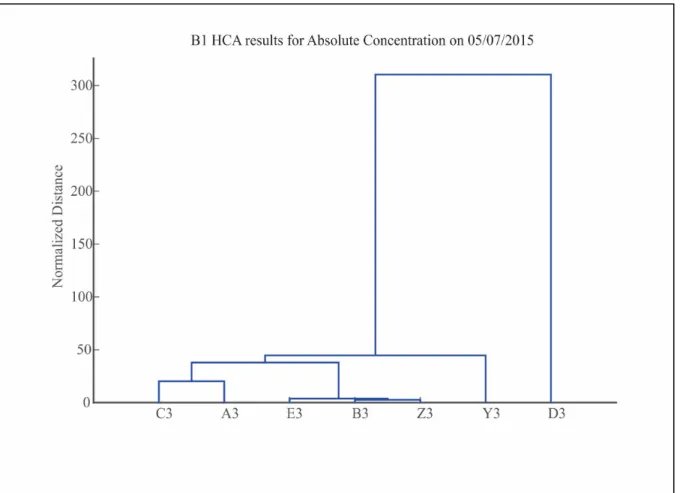
Hierarchical cluster analysis (HCA) is a statistical method that measures distance (or dissimilarity) in between columns of data matrices. In this study, it was used as a tool to identify tracers capable of separating end-members by similarity and to begin understanding hydrological processes by individual glacier. Dendrograms are the easiest visual
interpretation of HCA, leafs at the bottom represent specific samples, moving higher along the y-axis (normalized distance) leafs will fuse to one another through a node, these sets of branches are referred to as clusters. Based on the inputted dataset, clusters will form, and the higher the node the more disparate the samples, refer to figure 4.4 for better visualization. The clusters offered insights into the resemblance of chemical and physical properties of samples. Results were interpreted by visually analyzing the relationship of clusters in any given dendrogram.
Hierarchical cluster analysis (HCA) was carried out for each glacier’s end-members on both absolute concentrations and relative concentrations. Absolute concentrations give information of the similarity of chemical composition of end-members; samples that formed a cluster based on absolute concentration have similar chemistry and could belong to the same type (supraglacial, subglacial, etc.). Relative concentration eliminates the simple dilution effect and when results are clustered by origins, main contributors may be identified. For example, in a supraglacial sample clusters with the downstream sample, the main contributor would be the supraglacial stream.
A primary understanding of hydrological pathways and contribution was mandatory to ensure end-members were truly independent for the hydrochemical basin characterization method (HBCM) to be launched.
3.4 Quantitative Analysis
3.4.1 Hydrochemical Basin Characterization Method
The obtained set of tracers from the HCA analysis is then used in the hydrochemical basin characterization method (HBCM) to quantify relative contributions of end-members. For HBCM to be successful, a minimum of tracers must be selected, n-1 tracers for n end-members at a mixing point, for a maximum of n+5 tracers. The relative contribution of each
end-member is estimated using an over-parameterized set of mass balance equations (equation 3.6) (Baraer et al., 2009; Sinclair, 2014).
= ∑ ( ) + (3.6)
Where Ctot j is the relative concentration of the tracer j at a mixing point, n is the total number
of end-members, i is the end-member, Cij is the relative concentration of tracer j in the
end-member i, Qi is the proportion of end-member present in the total discharge, εj is the
accumulated error, finally Qtot is the total discharge at the mixing point (Baraer et al., 2009).
To obtain the best results from over-parameterization there should more tracers than end-members.
HBCM runs for each mixing point all possible combinations of tracers, based on a quasi Monte Carlo approach, and solves the eq 3.6 for the variable by minimizing the cumulative residual error ∑ , where m is the number of tracers considered (Baraer et al., 2009).
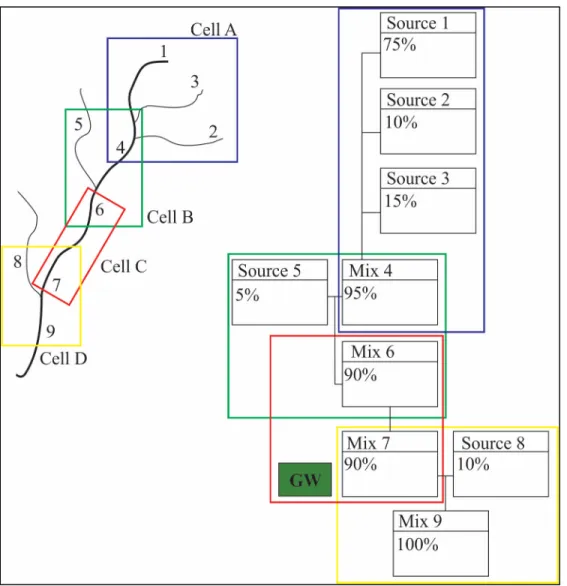
Figure 3.1 Illustration of HBCM’s geographic coverage of a hypothetical watershed: on the left is the hypothetical watershed (black lines represent the main stream and its tributaries, numbers represent sampling points); on the right is the corresponding schema for
HBCM where sampling points are separated into cells
In order to comprehend the visual representations of HBCM results, we must first understand the cells. Several types of cells can be distinguished. A two point cell (eg. cell C) is representative of two samples taken on a portion of the stream where there is mixing occurring with non-identified sources, referred to as groundwater sources (GW). A three point cell (eg. cell B or D), also referred to as a triple point, and represents two visibly large sources mixing into one. In this case, no other source of water contributes to the downstream sample. A third type of cell is similar to a triple point but instead of considering two