HAL Id: hal-01794094
https://hal.archives-ouvertes.fr/hal-01794094
Submitted on 17 May 2018
HAL is a multi-disciplinary open access
archive for the deposit and dissemination of
sci-entific research documents, whether they are
pub-lished or not. The documents may come from
teaching and research institutions in France or
abroad, or from public or private research centers.
L’archive ouverte pluridisciplinaire HAL, est
destinée au dépôt et à la diffusion de documents
scientifiques de niveau recherche, publiés ou non,
émanant des établissements d’enseignement et de
recherche français ou étrangers, des laboratoires
publics ou privés.
Feature Selection Framework for Multi-source Energy
Harvesting Wireless Sensor Networks
Marwa Lagha Kazdoghli, Fayçal Ait Aoudia, Matthieu Gautier, Olivier Berder
To cite this version:
Marwa Lagha Kazdoghli, Fayçal Ait Aoudia, Matthieu Gautier, Olivier Berder. Feature Selection
Framework for Multi-source Energy Harvesting Wireless Sensor Networks. IEEE Vehicular Technology
Conference (VTC-Spring), Jun 2018, Porto, Portugal. �hal-01794094�
Feature Selection Framework for Multi-source
Energy Harvesting Wireless Sensor Networks
Marwa Kazdoghli Lagha, Fayc¸al Ait Aoudia, Matthieu Gautier, Olivier Berder
Univ Rennes, CNRS, IRISA, France
Email: {marwa.kazdoghli-lagha, faycal.ait-aoudia, matthieu.gautier, olivier.berder}@irisa.fr
Abstract—Energy harvesting technologies are constantly evolv-ing to help power sensor network nodes. Rangevolv-ing from miniature power solar panels to micro wind turbines, nodes still express a deep need to harvest energies in order to keep both good perfor-mance level and energy autonomy. Recently, the simultaneous use of multiple sources has been proposed to tackle the time-varying characteristics of certain sources that can induce energy scarcity period and thus alter the node performance. In this context, this paper presents a methodology aimed at classifying the energy sources to choose the most efficient energy manager. As sensor nodes are embedded devices, it is necessary to ensure a balance between computational effort and classification accuracy. Feature extraction and selection phases can be processed and analyzed offline before deployment, and only a subset of features will be needed by the nodes to achieve efficient energy management. Simulations on real energy traces show that the proposed ap-proach achieves classification accuracy higher than 95% through the computation of 4 features only.
I. INTRODUCTION
The area of energy harvesting used for powering Wireless Sensor Network (WSN) nodes is an important research topic. Indeed, traditional battery-powered sensor nodes have many limitations [1] in terms of size, installation, maintenance and cost regarding many WSN applications, especially when long lifetime is required. Moreover, if the network is substantial or deployed in a harsh environment, batteries replacement can be impossible or too costly. To tackle this problem, a successful approach is to allow the nodes to continuously recharge their energy storage devices from environmental energy sources such as sunlight, wind, vibration, water flow. . . In energy harvesting WSNs, lifetime extension can be ensured thanks to an Energy Manager (EM) that adapts the sensor node parameters (e.g. throughput, sensing rate, transmission power, modulation schemes. . . ) to the harvested energy [2], [3].
A new trend in energy harvesting is to provide the node with the ability to be powered by several energy sources [4], [5]. In such multi-source energy harvesting systems, dedicated EMs must be designed to operate with the different sources. A first solution is the design of a source-independent EM such as RLman [6] that relies on reinforcement learning. On the other hand, if the node can benefit from some information about the energy source, it can either use one EM that is able to tune its parameters depending on the source (e.g. [7]) or work with different EMs (one EM per source). In such an approach, the node must identify its energy harvesting environment, which can be for instance different sources (e.g. wind/solar), different places (e.g. outdoor/indoor) or different
time (e.g. summer/winter). The identification of the energy environment of the node is the problem addressed in this paper and the proposed solution is to use a classification approach by extracting features from the harvested energy.
Different classes of energy that are available to be harvested must be defined before the WSN deployment depending on the available sources, hardware and application constraints and also the type of EM used. The classification process is performed by extracting features from the harvested energy profile. For simple scenarios, features could be intuitively selected. For instance, one can distinguish indoor and outdoor solar energies using the harvested energy variance, or periodic sources from others with no obvious periodic behavior (e.g. solar/wind) by computing the fundamental frequency of the harvested energy profile. However, this approach is not always efficient and feasible if the number of classes is important since the degree of similarity between classes increases. More-over, energy level is not used in this work as this feature’s value really depends on the harvesters used and the position of the nodes. Therefore, the goal of the paper is to propose a generic framework to select features to identify different classes. The contributions of this paper are:
- A framework to select features to classify different har-vested energy environment,
- An evaluation of different criterion to automatically select features in the context of energy harvesting,
- The application of the proposed framework on real traces (indoor light, solar and wind) and a fair comparison with an intuitive approach, the trade-off between the classifier complexity and accuracy is discussed.
The rest of this paper is organized as follows: Section II presents the energy harvesting classification process. In Sec-tion III, the feature extracSec-tion and feature selecSec-tion steps are detailed. Simulation results on real traces are exposed and discussed in Section IV and Section V is dedicated to the conclusions.
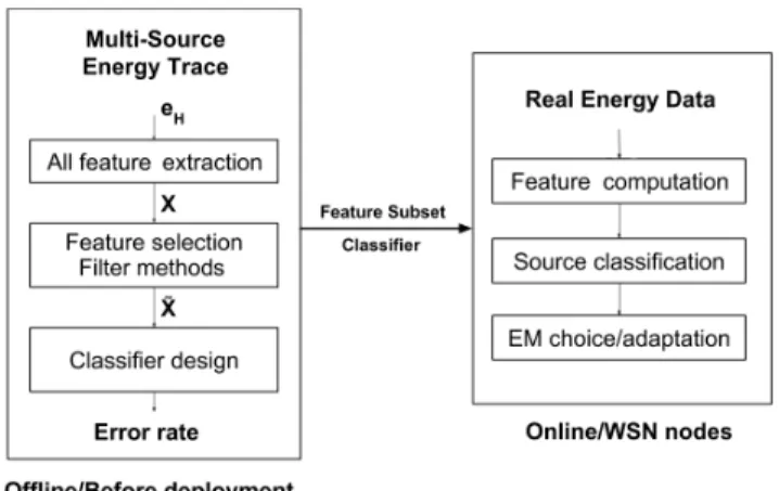
II. SOURCE CLASSIFICATION IN MULTI-SOURCEWSN In order to identify in which class falls the energy harvested by the node, it is worth presenting a global overview of the classification strategy. Fig. 1 shows the whole classification workflow, which mainly consists of two phases: (i) an offline processing is performed before the WSN deployment and designs the classifier structure and associated features to com-pute; (ii) an online processing is embedded in the node when
Fig. 1. Classification workflow.
being deployed, able to identify the harvested energy class that is currently present. For the offline classifier design, a set of energy traces is needed as input, each trace corresponding to a class. By denoting C the number of classes and N the number of energy samples, matrix EH of size C × N represents the
different energies able to be harvested by the node: EH= (eH1, eH2, . . . , eHC)
T
, (1) where eHi, i = 1, . . . , C is a 1 × N vector that contains the
harvested energy of class i.
The objective of the offline processing is to identify which class corresponds to the given energy harvesting eHi. To this
aim, two major steps have to be accomplished. The first one considers data transformation process from its raw values to feature domain values by executing feature extraction and selection techniques. Feature extraction transforms the raw data EH into a feature matrix X of size C × M with the M
the number of features. For a class, each feature is computed over the N energy samples. Feature selection aims to obtain a small subset of features ˜X of size C × P with P the number of selected features. This phase is extremely important since it seeks to decrease data dimensionality maintaining only the right features for the classification task. This step will be more detailed in the next section.
The second step consists in constructing a classifier from the extracted and selected features, calculated from the training energy data set, which contains information needed to char-acterize an energy source. Then, the objective, in regards to classification, is to explicitly determine, for each sample of the unknown energy data set, its membership to a class. Therefore, classification aims to train an algorithm which can identify the target class for any unknown energy vector e0H of size 1 × N . Many algorithms can be used to design the classifier, the most used are Decision Tree (DT), linear discriminant analysis and K-nearest neighbor. In this work, DT is specified as an algorithm of classification, due to its particular properties. Indeed, to challenge the embedded system constraints, DT insures a low complexity process as it could be implemented by using decision structures of ’IF . . . THEN’ type. Hence,
the DT structure that we used is a binary one in which each node can have zero, one or two child nodes. Each internal node represents a ’test’ on a feature, each branch represents the outcome of the test, and each leaf node represents a class label (decision taken after computing all attributes). The paths from root to leaf represent classification rules.
A binary DT is constructed through a process of dividing up the input space using a greedy approach called recursive binary splitting. This is a numerical procedure where all the values are lined up and different split points are tried and tested using a cost function. All input features and all possible split points are evaluated and chosen in a greedy manner based on the lowest cost function which is in our case Gini index. This criterion gives an idea of how good a split is by how mixed the classes are in the two groups created by the split.
Finally, both feature subset and classifier are embedded in WSN nodes. Online feature computation and classification are applied on real energy data to identify the energy environment. In our experimental setup, energy traces are split into a training set for the offline phase and a test set for the online phase, as explained in Section IV.
III. FEATURE EXTRACTION AND SELECTION
The feature extraction and selection from the matrix EH of
the different harvested sources are extremely important steps since it transforms raw data to a feature vector highlighting only useful information from the original input. The compu-tational effort required by the classifier can be therefore mini-mized, facilitating its implementation on embedded hardware. Feature extraction consists in processing statistical attributes (e.g. maximum, standard deviation. . . ) of an energy vector eHi. Hence, for each eHi (1 × N ), a vector xi (1 × M ) is
extracted. The element xi[k] of xi represents the kth feature
computed for class i. All features are computed over N energy samples. Based on related literature on classification methods [8]-[9], features are generally distinguished according to the domain in which they are calculated: time domain (e.g. minimum, maximum, standard deviation, entropy. . . ) and fre-quency domain (e.g. fundamental, harmonic, correlation. . . ).
At the outcome of the feature extraction step, data are represented by a large set of features and leaving out least informative features will reduce the size of the problem. The feature selection step aims at shrinking the number of features to P (P < M ) in order to reduce the computational effort of the system. Among different procedures of feature selection [10], filter methods will be used in the proposed framework as they achieve the lower complexity. Indeed, other methods, such as wrapper methods, iteratively include the classifier in the selection to improve accuracy of both selection and classification steps.
Filter methods process the features independently of the classifier by evaluating the relevance of the features based on a criterion function [11]. Once this ranking is computed by the criterion function, the least informative attributes are omitted and a feature set composed of the best P features is maintained. Number of criteria have been proposed for
filter-based feature selection [10]. In this work, the three most commonly used criteria are tested i.e. the Fisher score [12], the mutual information [13] and the ReliefF algorithm [14]. All these criteria are statistical, thus a large number of vectors eHi are needed to increase the efficiency of the selection
process. Fisher score:
Fisher criterion computes the degree of discrimination of the different classes. If there is a high correlation between one feature and the class of the data, then this latter is considered as a feature with high quality and will be useful for classification purposes. In the other case, the feature will be discarded. Fisher score for a feature k is defined by:
SF(k) = PC i=1ni(µki − µk)2 PC i=1ni(σik)2 , (2)
where µki and σki are respectively the mean and the standard
deviation of the kthfeature in the ithclass, ni is the number
of examples in the ith class and µk is the mean of the kth feature over all classes.
Mutual information:
Mutual information measures some kind of information that is mutual between a class and a feature. If Xi and Cl are
two random variables, which elements are respectively values of the ith feature and class label vector, then the mutual
information can be represented by:
SM I(i) = X xi X l P (Xi= xi, Cl= l) log P (Xi= xi, Cl= l) P (Xi= xi)P(Cl= l) , (3)
where P (Xi= xi, Cl= l) is the joint probability function of
Xi and Cl, and P (Xi= xi) and P (Cl= l) are the marginal
probability distribution function of Xi and Cl respectively.
ReliefF algorithm:
ReliefF’s target is to compute the merit of all features by evaluating the separation capabilities of randomly selected features. This can be seen in the proposed Algorithm 1. It is worth mentioning that this algorithm selects for each labeled vector of feature (instance) both the nearest same-class and opposite-class instance. Thus, features are ranked through their separation merit and this step is stored oftentimes for each chosen sample.
IV. SIMULATIONS RESULTS
A. Experimental setup
To fulfill autonomous energy harvesting classification goal, several data sets have been used from trusted sources. To be meaningful, the energy data used for the feature selection must be very long, i.e. it must last several years to cover potential seasonal effects. Therefore we have focused our work on devices that harvest three environmental sources (i.e. C=3): indoor light, solar and wind energies with sufficient data to be processed. Radiant light energy measurements are collected by
Algorithm 1 ReliefF Algorithm
Input: Training samples X = (x1, x2, . . . , xC)T where each
sample xi= (xi[1], xi[2], . . . , xi[M ])
1: ∀i, W [i] = 0
2: for t = 1 to T do . T is an input counter 3: Xk ← random sample
4: Xa ← nearest neighbor of Xk in the same class
5: Xb← nearest neighbor of Xk in a different class
6: for i = 1 to M do
7: W [i] = W [i] +|xki−xbi|
M T +
|xki−xai|
M T
8: return W: vector that contains the weight of each feature
Columbia University’s EnHANTs project and it is available in CRAWDAD repository [15], solar energy measurements come from the national solar radiation database [16] and wind energy data sets are extracted from National Wind Technology center [17]. The provided data sets are raw (i.e. irradiance of indoor light and solar energy, speed of wind energy), and therefore converted into energy data. The range of the three aforementioned energies are nearly the same i.e. between 0 and 163.5 mWh making the classification of the three sources a challenging task.
The observations are measured at a sampling frequency of one hour over a total duration of 3 years. Hence, the total set is composed of 26280 samples per class, which is a very high number for classification purpose as it demands a high computational effort as well as a big memory storage capacity. Therefore, features extraction is extremely crucial as it aims to synthesize the data in the form of a feature vector and thus reduce dimensionality of the incoming data while highlighting the useful information from the original one. In practice, to construct the input matrix EH, we experimentally choose
N =48 as a good compromise between the dimensionality reduction and the accuracy of the classifier. Indeed, for solar and indoor light energy class, there is a kind of cyclic trend which is not the case for wind energy which is completely stochastic. Thus, some features as auto-correlation or Fast Fourier Transform (FFT) may highlight the characteristics of such energies.
For the proposed approach, a set of M =40 features is defined based on the related literature [10][11]. To proceed classification algorithm, we commonly use 66 % of our data for training phase (i.e. two successive years) and 33 % for the test data set (i.e. the last year). Therefore, with N =48, we get 365 matrices EH to train and design the classifier during the
offline phase.
B. Classification results 1) Intuitive approach:
In order to compare our proposed generic approach to an intuitive feature selection, two features that should have high discriminant capabilities were chosen and provided to DT classifier to identify the three classes. The second peak of the FFT may distinguish the periodic sources (i.e. indoor light
and solar) and chaotic one (i.e. wind) while standard deviation may differentiate the two periodic sources.
In Fig. 2, these two features are shown on a two dimensional scatter plot, showing how the features can contrast all the classes. We observe that standard deviation and second peak of the FFT provide a border separating between the different sources. Fig. 2 also shows the separator values computed by DT algorithm with these two features. The plot is quite predictable as standard deviation is used to quantify the amount of variation or dispersion of a set of data values. It measures how concentrated the data are around the mean. In our case, solar is the most sparse data and the figure shows a separation boundary between solar and other sources. This result can be explained by the diurnal cycle of the solar (sunlight and night). Additionally, the second peak of the FFT determines the periodicity aspect which helps discarding wind energy which is not cyclic apart from other traces.
Hence, the error rate of classification using these features is 0.114. Despite this technique helps in discriminating the three harvesting energies, in practice, the number of classes may be far larger than three (e.g. the same EM or at least same parameters will not be used for indoor light powered nodes if they are near or far from a window). Moreover, the work is generally done with a big set of features and human knowledge cannot select which subset is the best for classification.
2) Feature selection:
This section aims to outline the error rate of classification when using the proposed feature selection methods for DT classifier when the size P of the feature subset ranges from 1 to 40. Fig. 3 shows results of the incremental feature selection classification for the three different energy harvesting data sets. This figure demonstrates the variation of error curve as the number of features increases.
As shown in Fig. 3, the overall performance of Fisher score is better than mutual information and ReliefF algorithm. In
Fig. 2. Second peak of the FFT vs Standard deviation for the three sources (indoor light, solar and wind) and the associated DT separators.
Fig. 3. Error rate of classification for three feature selection methods associated to DT classifer.
particular, classification accuracy of Fisher score is lower than other methods for little number of features. As our context of application is sensor nodes, we need to find the best trade-off between computation complexity and classification performance. Fisher based feature selection is therefore the most appropriate method in this case.
With Fisher method, the two first features selected are the third peak value of the FFT and the standard deviation. This result is similar to the intuitive approach as standard deviation is selected by both methods. However, Fisher score selects the third peak of the FFT rather than the second since the energy profile waveforms are not a perfect sinusoid (and only two daily periods are considered to compute the FFT). With these two features, the resulted error rate is decreased by half compared the intuitive approach (from 0.114 to 0.059). However, classification performance can be improved down to 0.04 by using two additional features.
C. Comparison and discussion
To analyze the performance of feature selection methods and the intuitive one, we compare their error rate, the complexity of the feature computations and the complexity of the constructed DT. Thus, it was possible to find out which classifier is the best in our task at hand. As shown in Fig. 3, the error rate decreases gradually when the features number increases; however, there is a floor effect as the error rate with P =4 features is about 0.042 with Fisher method and almost 0.02 with P =40. Therefore, working with the first four features
Intuitive Filter methods
approach Fisher MI ReliefF Error rate 0.114 0.0421 0.0531 0.0659 Feature complexity O(N log N ) O(N log N ) O(N2) O(N log N )
DT complexity 3 44 45 47 TABLE I
seems to be a good trade-off between classification accuracy, computation and memory usage.
Hence, Table I details classification performance when working with the first 4 features selected by each feature selec-tion algorithm. The feature complexity is given as a funcselec-tion of N and depends on the selected features. The DT complexity is given in number of ’IF . . . THEN’ decision structures. Fisher method provides the most appropriate classifier for embedded application compared to the other filter methods owing to its lowest computational complexity for both feature calculation and DT complexity and its lowest error rate.
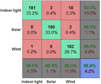
As a final result, the confusion matrix of the classifier obtained with the Fisher method (P = 4) is given in Fig. 4. It shows that the major disturbance is between indoor light and wind as the error rate of indoor light energy is the highest compared to solar and wind ones. Additionally, there is some confusion when identifying solar energy with indoor light energy. Nevertheless, the classifier helps distinguishing indoor light energy from other traces and the error rate of classification is the lowest in this case.
V. CONCLUSION
This paper presents a generic framework for identifying different harvested energy environments. Harvested energies have different trends and a generic classification process was carried out by processing raw data through feature extraction, feature selection, and then feeding into decision tree classifier. In the context of embedded sensor nodes, it is necessary to have a balance between the computational limitations of the node and classification performance. It is therefore essential to choose the minimal number of features using the appropriate features selection techniques. In the study case of our paper (indoor light, solar and wind classes), the Fisher criterion was used to extract only four features to feed the classifier, and these were sufficient to reach an error rate less than 5%,
Fig. 4. Confusion matrix for Fisher method (P = 4): the rows correspond to the identified class (Output Class), and the columns show the true class (Target Class).
therefore validating our framework. The latter will have to be further evaluated on other energy harvesting traces belonging to different classes, and eventually with mixed sources that are not intuitively separable. The gain brought by this framework has to be evaluated globally at a system point of view, taking into account the energy manager, and with measurements on real hardware platforms.
REFERENCES
[1] F. Wu, C. R¨udiger, and M. R. Yuce, “Real-time performance of a self-powered environmental iot sensor network system,” Sensors, vol. 17, no. 2, p. 282, 2017.
[2] T. N. Le, A. Pegatoquet, O. Berder, and O. Sentieys, “A Power Manager with Balanced Quality of Service for Energy-Harvesting Wireless Sensor Nodes,” in International Workshop on Energy Neutral Sensing Systems (ENSSys). Memphis, United States: ACM, Nov. 2014, pp. 19–24. [3] F. Ait Aoudia, M. Gautier, and O. Berder, “GRAPMAN: Gradual Power
Manager for Consistent Throughput of Energy Harvesting Wireless Sensor Nodes,” in IEEE International Symposium on Personal, Indoor, and Mobile Radio Communications, Hong Kong, China, Aug. 2015, p. 6. [4] A. S. Weddell, M. Magno, G. V. Merrett, D. Brunelli, B. M. Al-Hashimi, and L. Benini, “A survey of multi-source energy harvesting systems,” in IEEE/ACM Design, Automation Test in Europe Conference Exhibition (DATE), March 2013, pp. 905–908.
[5] P.-D. Gleonec, J. Ardouin, M. Gautier, and O. Berder, “Multi-source Energy Harvesting for IoT nodes,” in IEEE Online Conference on Green Communications (Online GreenComm), Nov. 2016.
[6] F. Ait Aoudia, M. Gautier, and O. Berder, “Learning to Survive: Achiev-ing Energy Neutrality in Wireless Sensor Networks UsAchiev-ing Reinforce-ment Learning,” in IEEE International Conference on Communications (ICC), Paris, France, May 2017.
[7] ——, “Fuzzy Power Management for Energy Harvesting Wireless Sensor Nodes,” in IEEE International Conference on Communications (ICC), Kuala Lumpur, Malaysia, May 2016.
[8] M. Christ, A. W. Kempa-Liehr, and M. Feindt, “Distributed and parallel time series feature extraction for industrial big data applications,” arXiv preprint arXiv:1610.07717, 2016.
[9] F. A. Borges, R. A. Fernandes, I. N. Silva, and C. B. Silva, “Feature extraction and power quality disturbances classification using smart meters signals,” IEEE Transactions on Industrial Informatics, vol. 12, no. 2, pp. 824–833, 2016.
[10] J. Tang, S. Alelyani, and H. Liu, “Feature selection for classification: A review,” Data Classification: Algorithms and Applications, p. 37, 2014. [11] G. H. John, R. Kohavi, K. Pfleger et al., “Irrelevant features and the subset selection problem,” in Machine learning: proceedings of the eleventh international conference, 1994, pp. 121–129.
[12] R. O. Duda, P. E. Hart, and D. G. Stork, Pattern classification. Wiley, New York, 1973.
[13] D. Koller and M. Sahami, “Toward optimal feature selection,” Stanford InfoLab, Tech. Rep., 1996.
[14] K. Kira and L. A. Rendell, “A practical approach to feature selection,” in Proceedings of the ninth international workshop on Machine learning, 1992, pp. 249–256.
[15] M. Gorlatova, A. Wallwater, and G. Zussman, “Networking Low-Power Energy Harvesting Devices: Measurements and Algorithms,” IEEE Transactions on Mobile Computing, vol. 12, no. 9, pp. 1853–1865, September 2013.
[16] S. Wilcox, “National solar radiation database 1991-2010 update: User’s manual,” Downloaded from http://rredc.nrel.gov/solar/old data/nsrdb/1991-2010/hourly/siteonthefly.cgi?id=722287.
[17] D. Jager and A. Andreas, “Nrel national wind technology cen-ter (nwtc): M2 tower; boulder, colorado (data),” Downloaded from http://www.osti.gov/scitech/servlets/purl/1052222.