HAL Id: hal-01354864
https://hal.inria.fr/hal-01354864
Submitted on 19 Aug 2016
HAL is a multi-disciplinary open access
archive for the deposit and dissemination of
sci-entific research documents, whether they are
pub-lished or not. The documents may come from
teaching and research institutions in France or
abroad, or from public or private research centers.
L’archive ouverte pluridisciplinaire HAL, est
destinée au dépôt et à la diffusion de documents
scientifiques de niveau recherche, publiés ou non,
émanant des établissements d’enseignement et de
recherche français ou étrangers, des laboratoires
publics ou privés.
Solving k-Set Agreement Using Failure Detectors in
Unknown Dynamic Networks
Denis Jeanneau, Thibault Rieutord, Luciana Arantes, Pierre Sens
To cite this version:
Denis Jeanneau, Thibault Rieutord, Luciana Arantes, Pierre Sens. Solving k-Set Agreement Using
Failure Detectors in Unknown Dynamic Networks. IEEE Transactions on Parallel and Distributed
Systems, Institute of Electrical and Electronics Engineers, 2016. �hal-01354864�
Solving k-Set Agreement Using Failure
Detectors in Unknown Dynamic Networks
Denis Jeanneau, Thibault Rieutord, Luciana Arantes, Pierre Sens
Abstract—The failure detector abstraction has been used to solve agreement problems in asynchronous systems prone to crash
failures, but so far it has mostly been used in static and complete networks. This paper aims to adapt existing failure detectors in order to solve agreement problems in unknown, dynamic systems. We are specifically interested in the k-set agreement problem.
The problem of k-set agreement is a generalization of consensus where processes can decide up to k different values. Although some solutions to this problem have been proposed in dynamic networks, they rely on communication synchrony or make strong
assumptions on the number of process failures.
In this paper we consider unknown dynamic systems modeled using the formalism of Time-Varying Graphs, and extend the definition of the existingΠΣx,yfailure detector to obtain theΠΣ⊥,x,yfailure detector, which is sufficient to solve k-set agreement in our model.
We then provide an implementation of this new failure detector using connectivity and message pattern assumptions. Finally, we present an algorithm usingΠΣ⊥,x,yto solve k-set agreement.
Index Terms—Distributed systems, Dynamic networks, Failure detectors, k-Set agreement
F
1
I
NTRODUCTIOND
YNAMICdistributed systems such as wireless or peer-to-peer networks pose new challenges to the field of distributed computing. In these systems, processes can join or leave the system during the run, and the communication graph evolves over time.In unknown networks, processes are lacking initial in-formation on system membership. Dynamic networks are often unknown, since it is difficult to know ahead of time which processes may join the system in the future.
Most of the existing distributed algorithms in the litera-ture were meant for static, known networks and make as-sumptions that are unrealistic in the context of unknown dy-namic networks: communication graphs are often assumed to be fully connected or even complete, and processes are expected to have full knowledge of the system membership. As a result, adapting existing protocols to unknown and/or dynamic networks is not trivial.
Agreement problems, and notably consensus, have been a lot less studied in dynamic networks than in static net-works. In this paper we are particularly interested in the k-set agreement problem, which is a generalization of the consensus problem such that 1-set agreement is consensus. In the k-set agreement problem, each process proposes a value, and some processes eventually decide a value while respecting the properties of validity (a decided value is a proposed value), termination (every correct process eventu-ally decides a value) and agreement (at most k values are decided).
Protocols solving consensus or k-set agreement have been proposed for dynamic systems, but they usually as-• D. Jeanneau, L. Arantes and P. Sens are with Sorbonne Universit´es,
UPMC Univ Paris 06, CNRS, INRIA, LIP6
• T. Rieutord is with INFRES, Telecom ParisTech
D. Jeanneau was supported by the Labex SMART, supported by French state funds managed by the ANR within the Investissements d’Avenir programme under reference ANR-11-LABX-65.
T. Rieutord was supported by the ANR project DISCMAT, under grant agreement N ANR-14-CE35-0010-01.
sume synchronous communications (as in [1], [2], [3], [4]) or make strong assumptions on the number of process failures [5].
We approach the k-set agreement problem from a failure detector perspective [6], [7]. Failure detectors provide pro-cesses with information on process failures. They have been used as an abstraction of system assumptions to circumvent the impossibility of solving consensus in asynchronous sys-tems prone to crash failures [8].
The ΠΣx,y failure detector was introduced in [9] and
is sufficient to solve k-set agreement in static networks (if and only if k ≥ xy) while being weaker than other known failure detectors which solve the same problem. However, this failure detector relies on information that is not avail-able in unknown networks: the list of all the participating processes. Additionally, traditional failure detectors rely on a full connectivity of the network graph, which is not available in a dynamic network.
In the current paper we extend the definition of ΠΣx,yin
order to obtain the ΠΣ⊥,x,yfailure detector, which is capable
of solving k-set agreement in unknown dynamic systems, and provide implementations of this new detector. We also adapt the set agreement algorithm of [9], [10] to solve k-set agreement using ΠΣ⊥,x,yon top of our model.
The model assumptions we propose to implement ΠΣ⊥,x,y are generic and expressed in terms of message
pattern, which allows our model to be applied to a range of systems. We also provide concrete examples of partial syn-chrony and failure pattern properties which are sufficient to ensure our generic assumptions.
The system is modeled using the formalism of the Time-Varying Graph (TVG), as defined in [11].
This paper thus brings the following main contributions: 1) The definition of the ΠΣ⊥,x,y failure detector as
an adaptation of ΠΣx,y to solve k-set agreement in
2) An algorithm implementing ΠΣ⊥,x,y in our model,
relying on connectivity and message pattern as-sumptions.
3) An algorithm solving k-set agreement in our model enriched with ΠΣ⊥,x,y, which is an adaptation of
the k-set agreement algorithm for static connected networks presented in [9], [10].
The remaining of the paper is organized as follows: Section 2 formally describes our system model. Section 3 presents the definitions of several failure detectors relevant to our work, and introduces the ΠΣ⊥,x,y failure detector.
Section 4 defines the different connectivity and message pattern assumptions that we rely on. In Section 5, we pro-pose an implementation of ΠΣ⊥,x,y. Section 6 presents an
algorithm solving k-set agreement with ΠΣ⊥,x,yfor k ≥ xy.
Section 7 presents the related work. Finally, Section 8 con-cludes the paper.
2
S
YSTEMM
ODEL2.1 Process Model
A finite set of n processes Π = {p1, ...pn} participate in
the system. The processes are synchronous (there is a bound on the relative speed of processes) and uniquely identified, although initially they are only aware of their own identities. Processes are not required to know the value of n.
A run is a sequence of steps executed by the processes while respecting the causality of operations (each received message has been previously sent). Processes can join and leave the system during the run (Π is the set of all pro-cesses that participate in the system at some point in time). Processes may also crash, and we make no difference be-tween a process that crashes permanently and a process that leaves the system permanently: in both cases the process is considered faulty in that run. A process that is not faulty is called correct. Note that this definition of faulty and correct processes is not exactly the traditional one. Indeed, correct processes can crash or leave the system, as long as they recover or come back later. Only processes that crash or leave permanently are considered faulty.
Correct processes can leave the system and come back infinitely often, but they can only crash and recover a finite number of times. The critical difference is that a process that leaves keeps its memory intact, whereas a crashed process does not.
The set of all correct processes is called C. We assume a bound f < n on the number of faulty processes in a run.
2.2 Communication Model
Processes communicate by sending and receiving messages. Communications are asynchronous: there is no bound on mes-sage transfer delays. Therefore, even though processes are synchronous, they do not cooperate in a synchronous way.
The system is dynamic, which means that nodes and communication links can appear or disappear during the run: therefore, the communication graph will change over time. The usual notion of path in the graph is not sufficient to define reachability in such a dynamic graph. To solve this issue, several solutions were proposed in the literature [1], [11], [12], [13]: we choose to model the communication graph using the Time-Varying Graph (TVG) formalism, as defined by Casteigts et al. in [11].
2.2.1 Time-Varying Graphs
Definition 1(Time-Varying Graph). A time-varying graph is a tuple G = (V, E, T , ρ, ζ, ψ) where
1) V = Π is the set of nodes in the system. 2) E ⊆ V × V is the set of edges.
3) T = N is a time span.
4) ρ : E × T → {0, 1} is the edge presence function, indicating whether a given edge e ∈ E is active at a given time t ∈ T . 5) ζ : E × T → N is the latency function, indicating the time taken to cross an edge e ∈ E if starting at given time t ∈ T . 6) ψ : V × T → {0, 1} is the node presence function, indicating whether a given node p ∈ V is present in the system at a given time t ∈ T . The edge presence function and the node presence function must be coherent: ∀t ∈ T , ∀pi∈ V , ∀e ∈ E, if e is
connected to pithen ψ(pi, t) = 0 =⇒ ρ(e, t) = 0.
G(V, E) is the underlying graph of G, and indicates which nodes have a relation at some time in T .
Note that processes do not know the values of the ζ function, which is only introduced for the simplicity of presentation. Since communications are asynchronous, the values of ζ are finite but not necessarily bounded.
The communication links between processes are not permanent: the ρ function indicates when a given edge is active. Therefore, the usual notion of path in the graph is not suited to TVGs: journeys are defined for this purpose.
Intuitively, a journey is a path over time. In order to transmit a message from process pi to process pjin a TVG,
it is not necessary for every edge on the path to be active at the time the message is sent: it is sufficient that there exists a path between between pi and pj such that all the edges
on the path are active in the right order at some time in the future.
Definition 2(Journey). A journey is a sequence of couples J = {(e1, t1), (e2, t2), ..., (em, tm)} such that {e1, e2, ..., em} is a
walk in G and:
∀i, 1 ≤ i < m : (ρ(ei, ti) = 1) ∧ (ti+1≥ ti+ ζ(ei, ti)) .
t1 is called departure(J ) and tm+ ζ(em, tm) is called
arrival(J ). We denote J(u,v)∗ the set of all the journeys starting at node u and ending at node v.
Consider the following example: a graph where E = V × V and every edge in the system is active in-finitely often (longer than the message transfer time), but no more than one edge is ever active at a time. In such a system, there are journeys infinitely often between every node and the connectivity is sufficient to solve complex problems such as consensus. However, at any given instant, the graph is partitioned into at least n − 1 independent subsets. This shows that similarly to paths, the usual notion of graph partitioning loses relevancy in TVGs: the number of partitions at a particular instant in the run is not a very useful parameter. Instead we are interested in the number of partitions over time: in the rest of the paper, we use the word partition to refer to a subset of the network that is isolated from the rest of the network for an arbitrarily long duration, and not just temporarily.
2.2.2 Communication primitive
Processes communicate exclusively by sending messages with a broadcast primitive. We are relying on a very simple
broadcast: when a process pi calls the broadcast primitive,
the message is simply sent to the processes that are currently in pi’s neighborhood, including pi. We do not require the
broadcast to provide advanced features such as message forwarding, routing, message ordering or any guarantee of delivery.
2.2.3 Channels
The channels are fair-lossy. Messages may be lost but, if the edge is active for the entire time of the message transfer, a message sent infinitely often will be received infinitely often. Messages may be duplicated, but a message may only be duplicated a finite number of times. No message can be created or altered. We make no assumption on message ordering and do not require channels to be FIFO.
3
F
AILURED
ETECTORSFailure detectors ([6]) are distributed oracles that provide processes with unreliable information on process failures, often in the form of a list of trusted process identities. This information is unreliable in the sense that the failure detec-tor may erroneously consider a correct process as faulty, or vice versa, but will attempt to correct these mistakes later. Each failure detector class ensures some properties on the reliability of the failure information. A failure detector is an abstraction of the system assumptions used to solve a given problem.
The failure detector abstraction has been investigated as a way to circumvent the impossibility result of [8] and solve consensus in asynchronous systems prone to crash failures [7]. Our goal in this paper is to adapt this solution to solve k-set agreement in dynamic systems.
Traditionally, failure detectors are used in system mod-els considering static and fully connected communication graphs. These connectivity properties are usually presented as properties of the system model rather than the failure detector augmenting it. When considering a much weaker system model such as a dynamic network, solving any non-trivial problem still requires the assumption of a certain degree of graph connectivity, as not much can be done in a system where no communication link is ever active. Studying dynamic systems means considering the level of temporal connectivity required to solve a specific problem: using a generic and strong connectivity assumption would defeat that purpose. Instead, the goal should be to use a weak connectivity assumption that is still sufficient to solve the problem. Therefore, to solve a given agreement problem, two things are necessary: (1) a failure detector and (2) a connectivity assumption.
But if connectivity assumptions must be added to the system model in addition to the failure detector, then it cannot be said that the failure detector is sufficient to solve the problem. For this reason, and because in a dynamic system the required level of connectivity is as dependent on the problem as the required failure detector, we con-sider that failure detectors for dynamic systems should include connectivity properties. Adding these connectivity properties should not be seen as strengthening the failure detectors: they are still weaker than the assumption of a fully connected, static communication graph.
Additionally, our system model considers an unknown network where processes have no information on system membership at the beginning of the run. A way to circum-vent this issue was proposed in [14] in the form of the Σ⊥
failure detector
Our approach is based on the ΠΣx,y failure detector
of [9], augmented with connectivity properties and ex-tended with the method of [14] in order to obtain a failure detector sufficient to solve the k-set agreement problem in unknown dynamic systems.
3.1 The Quorum Failure Detectors
The quorum failure detector Σ, [15], provides every process with sets of process identities (called quorums) such that any two quorums output by Σ at any time necessarily in-tersect. Additionally, Σ requires that all quorums eventually contain only correct processes.
The Σk failure detector, [16], is a generalization of Σ
meant to solve k-set agreement. Similarly to Σ, Σk provides
processes with eventually correct quorums, and at least two out of any k + 1 quorums must intersect. It is easy to see that Σ = Σ1.
Intuitively, Σk prevents the network from partitioning
into more than k independent subsets. Note that in the case of a dynamic network, this statement only applies to partitions over time: the network may still be instantaneously partitioned into any number of subsets at any given instant. In message passing systems, Σ is necessary to solve consensus ([15]) and Σk is necessary to solve k-set
agree-ment ([16]).
The intersection property of Σ and Σk must hold over
time, which means that if a process queries its failure detec-tor before any communication has taken place, the returned quorum must intersect with the quorums formed by other processes later in the run. In known networks, implementa-tions of Σ traditionally solve this issue by returning Π as a quorum at the beginning of the run [15]. This is not an op-tion in unknown networks where knowledge of the system membership is only established through communication.
The Σ⊥ failure detector, [14], is an adaptation of Σ for
unknown networks: instead of returning a quorum, Σ⊥can
also output the default value ⊥ whenever the knowledge necessary to form a quorum has not been gathered yet.
In order to solve k-set agreement in unknown dynamic networks, we define the Σ⊥,k failure detector, which
com-bines the properties of Σk and Σ⊥. It also includes a
con-nectivity property which replaces (and is weaker than) the assumption of a static and complete network.
The Σ⊥,kfailure detector provides each process pi with
a quorum denoted qriτ (which is either a set of process
identities or the special value ⊥) at any time instant τ . For the convenience of the presentation, we introduce the following definition:
Definition 3(Recurrent neighborhood). The recurrent neigh-borhood of a correct process pi, denoted Ri, is the set of all correct
processes whose quorums intersect infinitely often with pi’s
quo-rums. ∀pi∈ C, Ri = {pj∈ C |∀τ , ∃τi, τj ≥ τ : qriτi 6= ⊥ ∧ qrτj j 6= ⊥ ∧ qr τi i ∩ qr τj j 6= ∅}.
Note that pj∈ Ri is an equivalence relation between
pi and pj. By definition, ∀pi ∈ C : pi ∈ Ri and therefore
We say that a correct process pican reach another correct
process pj if, provided that pi sends messages infinitely
often, pj receives them infinitely often.
Σ⊥,k is defined by the self-inclusion, quorum liveness,
quorum intersection and quorum connectivity properties.
Property 1(Self-inclusion). Every process includes itself in its non-⊥ quorums. ∀pi∈ Π, ∀τ : (qrτi 6= ⊥) =⇒ (pi∈ qriτ) . Property 2(Quorum liveness). Eventually, every correct pro-cess stops returning ⊥ and its quorums only contain correct processes. ∃τ , ∀pi∈ C, ∀τ0≥ τ : qrτ
0
i 6= ⊥ ∧ qrτ
0
i ⊆ C . Property 3(Quorum intersection). Out of any k + 1 non-⊥ quorums, at least two intersect.
∀τ1, ..., τk+1∈ T , ∀id1, ..., idk+1∈ Π, ∃i, j : 1 ≤ i 6= j ≤ k + 1 : (qrτi idi 6= ⊥ ∧ qr τj idj 6= ⊥) =⇒ (qr τi idi∩ qr τj idj 6= ∅) .
Property 4 (Quorum connectivity). Every correct process pi
can reach every process in Ri.
Σkand Σ⊥were defined with only 2 properties (liveness
and intersection). Self-inclusion is a property added to Σx
and ΠΣxby the authors in [9] for the sake of the simplicity
of algorithm proofs, and it is trivially implemented by the algorithms we present in the rest of the paper. Quorum con-nectivity is the property added to deal with the dynamicity of the network.
Intuitively, the quorum connectivity property means that processes belong to the same partition as their recur-rent neighborhood. Note that ∀pi, pj ∈ C : pi∈ Rj =⇒
pj∈ Ri, thus quorum connectivity enables two-way
com-munication between piand pj.
This property is not very costly, since most intuitive fail-ure detector implementations would already require some level of connectivity between processes in a quorum in order to form the quorums. This is the case for the Σ⊥,kalgorithm
we present in Section 5, which will not require any addi-tional assumption to implement quorum connectivity.
3.2 The Family of Failure Detectors ΠΣx,y
Although Σkis necessary to solve k-set agreement, it is not
sufficient. It has been shown in [10] that k-set agreement can be solved in static asynchronous networks with hΣx, Ωyi,
with k ≥ xy, where Ωy is the eventual anti-leader
detec-tor [17]. It was shown in the same paper that if n ≥ 2xy, then there is no hΣx, Ωyi-based k-set algorithm for k < xy,
which means that the k ≥ xy requirement is tight.1
However in [9], Most´efaoui, Raynal and Stainer intro-duce the ΠΣx,y failure detector and prove that it is strictly
weaker than hΣx, Ωyi for 1 < y < x < n while still being
strong enough to solve k-set agreement with k ≥ xy. In-terestingly, ΠΣx,y is defined incrementally based on the
properties of Σx. Therefore, an algorithm for Σx(or Σ⊥,x, in
our case) can easily be extended to implement ΠΣx,y(resp.,
ΠΣ⊥,x,y), with an additional assumption.
The authors in [9] provide an intuitive description of ΠΣx,y. ΠΣx,1 (1) prevents the system from partitioning
into more than x partitions with the properties of Σx and 1. This result can also be proved using the impossibility of k-set agreement theorem ([18]), the premise of which applies ifk < xy.
(2) guarantees that the processes of at least one of these subsets agree on a common leader. ΠΣx,y can be seen as
y independent instances of ΠΣx in which (2) has to be
guaranteed in only one of these instances.
We define ΠΣ⊥,x,y as an extension of ΠΣx,y that
in-cludes the properties of Σ⊥,xand is capable of solving k-set
agreement in unknown dynamic systems.
3.3 The Family of Failure Detectors ΠΣ⊥,x,y
Similarly to [9], ΠΣ⊥,x,y is defined incrementally: ΠΣ⊥,xis
defined firstly.
3.3.1 The failure detector ΠΣ⊥,x
At any time instant τ , ΠΣ⊥,xprovides each process piwith
a quorum denoted qriτ (which is either a set of process
identities or the special value ⊥) and a leader denoted leaderτ
i (which is a process identity).
ΠΣ⊥,x is defined by the following properties: • Self-inclusion
• Quorum liveness
• Quorum intersection • Quorum connectivity • Eventual partial leadership
Σ⊥,x
First, we define an eventual partial leader as follows:
Definition 4 (Eventual partial leader). An eventual partial leader pl is a correct process such that every process in the
recurrent neighborhood of pleventually recognizes plas its leader
forever. pl∈ C ∧ ∀pi∈ Rl, ∃τ , ∀τ0≥ τ : leaderτ
0
i = pl .
We denote L the set of all eventual partial leaders.
Property 5 (Eventual partial leadership). For every correct process pi, there is an eventual partial leader plthat can reach pi.
The original eventual partial leadership property used in [9] simply requires the existence of an eventual partial leader in the system. Our version of the property similarly implies that L 6= ∅ (since C 6= ∅), but also implies that each correct process must be reachable by one eventual partial leader (which, depending on the level of connectivity, may require more than one leader). In a static and connected network, both properties are equivalent: a single eventual partial leader is necessary and sufficient to fulfill the prop-erty, since the connected communication graph enables this single leader to reach every correct process.
In a k-set agreement algorithm, the eventual partial lead-ers are the processes that are ensured to decide eventually. In order to ensure termination, the deciding leaders must, therefore, be able to inform the rest of the system of their de-cision. However, in a dynamic network, the mere existence of an eventual partial leader does not provide the latter with the necessary connectivity to ensure termination. This is why in dynamic networks, our eventual partial leadership property is stronger than the original one and imposes the required connectivity.
The eventual partial leadership property implies a trade-off between the number of eventual partial leaders in the system and graph connectivity. On one hand, if there is a single leader in the system, then this leader must be able to reach every correct process in the system. On the other
hand, if the communication graph is partitioned, then there must be at least one local leader per partition.
Such a trade-off implies that the eventual partial leader-ship property does not prevent the system from being parti-tioned into up to n partitions over time, provided that every correct process is its own eventual partial leader. However in this scenario it would be impossible to verify the quorum intersection and quorum connectivity properties.
3.3.2 The failure detector ΠΣ⊥,x,y
The definition of ΠΣ⊥,x,yis the same as ΠΣx,yin [9], except
that it uses ΠΣ⊥,xinstead of ΠΣx. ΠΣ⊥,x,ycan be seen as y
instances of ΠΣ⊥,xrunning concurrently.
ΠΣ⊥,x,y provides each process pi with an array
F Di[1..y] such that for each j, 1 ≤ j ≤ y, F Di[j] is a
pair containing a quorum F Di[j].qr and a process index
F Di[j].leader. The array satisfies the following properties: Property 6 (Vector safety). ∀j ∈ [1..y] : F Di[j].qr satisfies
the self-inclusion, liveness, intersection and quorum connectivity properties of ΠΣ⊥,x.
Property 7(Vector liveness). ∃j ∈ [1..y] : F Di[j] satisfies the
eventual partial leadership property of ΠΣ⊥,x.
The idea is to reduce the cost of the system assumptions: the liveness property only needs to be verified by one out of a set of y instances of the detector.
The authors in [9] prove that for 1 ≤ y ≤ n − 1, ΠΣ1,y
is as strong as hΣ1, Ωyi. This shows that the y parameter of
ΠΣx,y (and ΠΣ⊥,x,y) is comparable to the y parameter of
Ωy.
ΠΣ⊥,x,y is sufficient to solve the k-set agreement
prob-lem in our model if k ≥ xy. We will prove this statement by providing a k-set agreement algorithm relying on ΠΣ⊥,x,y
in Section 6.
4
A
SSUMPTIONSIn this section we present some system assumptions. The algorithms presented in Section 5 will then list the assump-tions from this section on which they rely.
4.1 Time-Varying Graph Classes
In addition to defining the formalism of the TVG, Casteigts et al. present in [11] a number of TVG classes which provide different levels of connectivity assumptions. We are particu-larly interested in class 5.
Definition 5 (Class 5: recurrent connectivity [11]). All pro-cesses can reach each other infinitely often through journeys. ∀u, v ∈ Π, ∀τ , ∃J ∈ J∗
(u,v): departure(J ) > τ .
This connectivity assumption does not exactly fit our purpose. On the one hand, it is too strong. It implies a global connectivity between any two processes in the sys-tem, which is not necessary to solve k-set agreement, since the problem can be solved in a system partitioned into k subsets.
On the other hand, class 5 is too weak since it relies on the notion of journey, which is insufficient to ensure the transmission of messages. Even if a journey exists between pi and pj, there is no guarantee that a message sent by pi
can reach pj. In fact, even if the edge between pi and pj
is active infinitely often and the message is sent infinitely often, the message might always be sent in between two activation periods of the edge, thus never crossing it. To solve this problem, G ´omez-Calzado et al. defined in [19] the notion of timely journeys for the case of synchronous systems. We extend this solution into γ-journeys for the case of asynchronous communications.
Definition 6 (γ-Journey). A γ-journey J (where γ > 0 is a time duration) is a journey such that every node on the path can wait up to γ units of time after the next edge becomes active before forwarding the message. Since the message may be sent at any time during the γ time window and the channel latency may vary during that time, the edge must remain active long enough for the worst case duration.
- ∀i, 1 ≤ i ≤ |J |, eistays active from time tiuntil, at least, time
ti+ max0≤j≤γ{j + ζ(ei, ti+ j)} .
- ∀i, 1 ≤ i < |J |, ti+1≥ ti+ max0≤j≤γ{j + ζ(ei, ti+ j)} .
With a γ-journey, processes are given an additional time window of γ units of time to send the message. In [19], this time was used to detect the activation of the edge. This solution is appropriate for point-to-point communications in a known network, since it allows the emitter of the message to resend the message to the receiver whenever the edge appears again. However this is not helpful in a unknown non-complete network where we have to rely on blind broadcasts and forwarding to propagate information.
Instead, we use the additional time window provided by γ-journeys as an upper bound on the time between two emissions of the message. This explains the need for synchronous processes: each process should be able to re-peatedly send every message at least once every γ units of time.
Provided that processes receive their own broadcasts within γ time instants and then rebroadcast it, we can be sure that every message is sent at least once every γ instants. If there is infinitely often a γ-journey from pito pj, then
pican reach pj.
We call J(u,v)γ the set of all the γ-journeys from u to v. Using class 5 as a starting point, we define TVGs of class 5-(α, γ) as follows. γ is the time duration parameter of γ-journeys, and α is a parameter defining how many processes each correct process is ensured to communicate with.
Assumption 1(Class 5-(α, γ): (α, γ)-recurrent connectivity). Every correct process can reach and be reached through γ-journeys infinitely often by at least α correct processes.
∀pi∈ C, ∃Pi⊆ C, |Pi| ≥ α, ∀t ∈ T , ∀pj ∈ Pi,
∃Ji∈ J(pγ
i,pj): departure(Ji) ≥ t ∧
∃Jj ∈ J(pγ
j,pi): departure(Jj) ≥ t .
This assumption is parametrized by the two values α and γ. A low γ value weakens the connectivity assump-tion by allowing shorter time windows for the journeys, but implies that processes must be able to send messages more often to ensure that a message is sent within the shorter window. On the other hand, a high γ value reduces the number of journeys that are qualified as γ-journeys, thus strengthening the connectivity assumption, but accepts slower processes.
The α parameter also presents a trade-off: class 5-(α, γ) indirectly implies that there must be at least α correct
processes in the system. As a result, a high α value will result in a strong assumption on the number of process failures which can be costly in a dynamic system. A low α value would strengthen the message pattern assumptions presented in the next section.
Class 5-(α, γ) also implies that all correct processes must know a lower bound of α.
The assumption of a TVG of class 5-(α, γ) means that correct processes are able to communicate infinitely often with a subset of α correct processes. This property ensures that correct processes will not wait for messages forever, which enables our algorithm to ensure the quorum liveness property. Additionally, if the algorithm ensures that every correct process pi eventually only forms quorum from the
Piset, then class 5-(α, γ) also ensures quorum connectivity.
4.2 Message Pattern Assumptions
In this section we present message pattern assumptions, as defined by Most´efaoui et al. in [20]. The message pattern model consists in assuming some properties on the relative order of message deliveries. If processes periodically wait for a certain number of messages, the idea is to assume that the message sent by some specific process will periodically be among the first ones received.
In order to express our message pattern assumptions, we will assume that the distributed algorithm executed by processes uses a query-response mechanism. Processes periodically issue query messages, to which other processes will respond.
The principle of our failure detector algorithm revolves around processes repeatedly issuing a query and then wait-ing for responses from α processes: α is therefore the mini-mum size of quorums returned by the algorithm. This does not necessarily constitute an assumption on the number of failures, since α might be chosen equal to 1. This α is the same parameter we used to define TVGs of class 5-(α, γ) which ensures that correct processes will not wait for messages for infinitely long.
We call response set the set of the first α processes whose response to a given query issued by process piare received
first by pi.
4.2.1 Assumptions for Quorum Intersection
The assumption of a TVG of class 5-(α, γ) is not sufficient to ensure the quorum intersection property. In [10], Bouzid and Travers proposed a method to implement quorums: if processes repeatedly wait for messages from at least b n
k+1c + 1 processes before using the new list of processes as
their quorum, then the size of quorums alone is sufficient to ensure intersection. This method implies that there must be at least bk+1n c + 1 correct processes in the system, otherwise processes would wait forever, thus preventing liveness.
In a dynamic system where processes are expected to join and leave the system, such an assumption on the number of process failures seems too costly. For this reason we prefer to rely on the message pattern approach.
The following assumption is sufficient for our algorithm to implement quorum intersection. It was obtained by gen-eralizing the assumption used for the case k = 1 in [14].
Fig. 1. Example of multiple winning quorums (m = k = 3).
Assumption 2(Generalized winning quorums). ∃m ∈ [1, k] and ∃Qw1, ..., Qwm⊆ Π (called winning quorums). Each
win-ning quorum Qwiis associated with a number wi≥ 1 (called the
weight of Qwi) such that Pmi=1wi≤ k. ∀p ∈ Π, every time p
issues a new query, ∃i ∈ [1, m] such that Qwi6= ∅ and out of
the first α processes from which p receives a response, at least b|Qwi|
wi+1c + 1 of them are in Qwi.
Intuitively, Assumption 2 requires that there are m sets of processes, the winning quorums, that answer faster than others, i.e., faster enough for parts of these sets to always be included in every response set. In addition, every time a correct process issues a query, connectivity must allow for part of one of these winning quorums to receive and respond to the query.
Note that winning quorums do not necessarily corre-spond to quorums returned by the failure detector at some point: instead they are sets of processes that have a tendency to be included in response sets.
The weight wi of a winning quorum is a parameter
which states which proportion of the winning quorum must be included in response sets. A winning quorum of weight 1 must be included in strict majority by a response set, whereas winning quorums of higher weights can be included in smaller proportions. The sum of all winning quorum weights is limited by k.
It is interesting to consider some extreme instances of this assumption. The first extreme is m = k: in this partic-ular case, all winning quorums are necessarily of weight 1, and therefore each response set must include a strict ma-jority of one of the winning quorums. Since each response set includes the strict majority of one out of k winning quorums, it is easy to see that out of any k + 1 response sets, at least two will necessarily intersect.
Fig. 1 shows an example for m = k = 3 in which win-ning quorums are represented by dashed red circles. Each solid black circle represents a response set. Note that out of any 4 response sets, at least 2 intersect.
Another extreme case is m = 1 and w1= k. In this
particular case, all response sets must contain a small part of a single winning quorum.
Fig. 2 shows an example for m = 1 and k = 3. Similarly to Fig. 1, the winning quorum is represented by a dashed red circle, and response sets are represented by solid black circles. Once again, 2 out of any 4 response sets intersect.
The flexibility in the second example lies in which part of the winning quorum will be included in each response set, while the flexibility in the first example lied in which winning quorum would be included in majority by each response set.
Fig. 2. Example of a single winning quorum (m = 1, k = 3).
Assumption 2 implies that there is at least one winning quorum Qwisuch that at least b|Qwiwi+1|c + 1 of the processes
in Qwi are correct. If α = b|Qwiwi+1|c + 1 = 1, then there is no
assumption on the number of failures but |Qwi| < wi+ 1,
which only leaves minimal flexibility on the processes that must be included in every response set, thus strengthening the message pattern assumption. On the other hand if |Qwi|
is high (and therefore α is high), the number of failures is limited but each response set must contain a subset of a larger set, which allows for more flexibility in the message pattern.
4.2.2 Assumption for Eventual Partial Leadership
In order to ensure the eventual partial leadership property, processes need to identify a local leader. Once again we choose to rely on a message pattern assumption. Since the eventual partial leadership property is supposed to be implemented on top of Σ⊥,x, we can use the notion of
quorum to define this new assumption.
Additionally, we use the order of processes in quorums to single out the leader. For this purpose we assume that processes in a quorum are totally ordered. Any specific ordering can be used: a natural choice would be to use the order in which the processes were added to the quorum. Another simple choice would be to order according to process identifiers. For a process pi and a quorum qr, if
pi∈ qr, then we denote by pos(pi, qr) the position of pi in
qr according to the chosen total order. If piis the first process
in qrτj, then pos(pi, qrτj) = 1. In this particular case, we say
that piis the candidate of pjat time τ .
We define our potential eventual partial leaders as fol-lows:
Definition 7(Eventually winning process). A correct process plis called an eventually winning process if there is a time τ such
that after τ, ∀τ0≥ τ , ∀pi ∈ Rl\{pl} :
1) plis present in every quorum formed by pi. pl∈ qrτ
0
i .
2) pl’s identity is always positioned in pi’s quorum before
the identities of other processes in Ri. ∀pj ∈ Ri\{pl, pi} :
pos(pl, qrτ
0
i ) < pos(pj, qrτ
0
i ) .
3) In every quorum formed by pi, there is another process that
also belongs to Rl. ∃pj∈ Rl\{pl, pi} : pj∈ qrτ
0
i .
Point (1) means that after some time, pl must be fast
enough for its responses to arrive in time to take part in every local quorum.
The implication behind (2) depends on the chosen order-ing method. If processes are ordered by date of addition to the quorum, then (2) implies that after some time, plmust
be faster than the rest of the recurrent neighborhood of pi.
If processes are ordered by process identities, plmust have
the smallest process identity in the recurrent neighborhood. It is easy to see why (1) and (2) are useful: if pl is part
of every quorum and is singled out by the quorum order, then processes in Rl can reliably select their candidate as
the leader.
Note that (2) excludes the case pi= pj, since otherwise
pl would have to be placed before pi in pi’s quorums. If
processes are ordered by date of addition to the quorum, this expectation would be very unrealistic since receiving its own message is a local computation and should therefore be faster than receiving pl’s message.
Point (3) requires that processes in Rl must not only
communicate with pl but also with each other to some
extent, which enables them to share the information that plis their candidate.
Note that (3) also requires the processes pl, pi and pj to
be distinctly defined: therefore, in order for an eventually winning process to exist, there must be at least 3 correct processes in the system (f ≤ n − 3). Since pl, piand pjmust
be included in the same quorums, α must also be equal to 3 or greater.
We call W the set of all eventually winning processes. We can now formulate the assumption that will enable our failure detector algorithm to ensure the eventual partial leadership property:
Assumption 3 (Eventually winning γ-sources). For every correct process pi, there is an eventually winning process pl
such that there is infinitely often a γ-journey from pl to pi.
∀pi∈ C, ∃pl∈ W , ∀τ : ∃J ∈ J γ
(pl,pi)∧ departure(J ) > τ .
Our ΠΣ⊥,x algorithm will ensure that eventually
win-ning processes are eventual partial leaders. As a result, this assumption will be sufficient to ensure the eventual partial leadership property.
4.3 Summary of assumptions
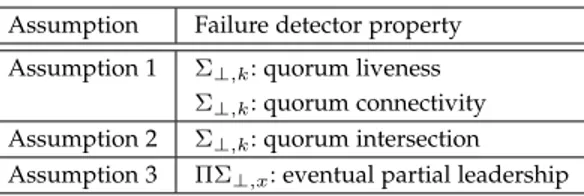
Table 1 summarizes the assumptions presented in this sec-tion and the failure detector properties that they enable us to implement.
TABLE 1
Assumptions for failure detector implementations Assumption Failure detector property Assumption 1 Σ⊥,k: quorum liveness
Σ⊥,k: quorum connectivity
Assumption 2 Σ⊥,k: quorum intersection
Assumption 3 ΠΣ⊥,x: eventual partial leadership
The self-inclusion property of Σ⊥,k is absent from this
table because it does not require any assumption and will simply be ensured through algorithmic properties.
4.4 Implementation of Message Pattern Assumptions
Assumptions 2 and 3 are very abstract and it can be difficult to judge at first glance how likely they are of being verified in a real network. This is because we attempt to isolate assumptions that are specifically as close as possible to the minimum model strength required to ensure that our algo-rithm implements the ΠΣ⊥,x,yfailure detector. The message
pattern model allows us to do this while keeping our model generic and applicable to different networks.
In this section we provide examples of more traditional assumptions that are sufficient to ensure Assumptions 2 and 3.
4.4.1 Implementation of Assumption 2
A simple and intuitive method is to assume that |C| ≥ b n
k+1c + 1. In this case, Assumption 2 is trivially
ver-ified with m = 1, w1= k and Qw1= Π. This implies that
α ≥ b n
k+1c + 1: the minimal size of quorums formed is then
sufficient to ensure intersection. This particular case is the method used to implement Σkin static networks in [10].
Another method would be to use a partial synchrony assumption. For a given duration ∆, let us call ∆-journey a γ-journey J such that arrival(J ) − departure(J ) ≤ ∆. We then separate Π into two subsets: slow processes and fast processes. A slow process pi is a process such that
there is never a ∆-journey from pi to any correct process
pj∈ C\{pi}. Fast processes are all other processes and Q is
the set of all correct fast processes. The assumption is then that for any correct process piand any time instant, there are
∆-journeys linking pi to at least bk+1|Q|c + 1 processes from
Q. Assumption 2 is then verified with m = 1, w1= k and
Qw1= Q.
4.4.2 Implementation of Assumption 3
One way to ensure Assumption 3 is that there is a correct subset Q of the system that is constantly connected and recognizes a leader pl, that can reach the entire system
infinitely often. The leader must be known from the other processes in Q from the start (it can simply be the lowest process identifier in Q, for example). When a process in Q issues a query, the communication layer for that process will then wait for a response from pl and a response from
another process in Q before delivering any other response. This is sufficient to ensure that plis the first process in every
quorum formed in Q, and that processes in Q communicate with each other to a sufficient extent.
4.4.3 Practical issues
From a practical point of view, some types of networks are particularly adapted to ensure Assumptions 2 and ??. In wireless mesh networks ([21]), the nodes move around a fixed set of nodes and each mobile node eventually connects to a fixed node. Wireless sensor networks ([22]) can be organized in clusters; one node in each cluster is designated the cluster head. Messages sent between clusters are routed through the cluster heads of the sending and receiving clus-ters. An infra-structured mobile network ([12]) is composed of Mobile Hosts (MH) and Mobile Support Stations (MSS). A MH is connected to a MSS if it is located in its transmission range, and two MHs can communicate only through MSSs.
In each of these network models, there is a privileged subset of powerful nodes (fixed nodes, cluster heads, MSSs) that can be used as a winning quorum to satisfy Assump-tion 2 or as the neighborhood Rl of an eventual winning
process plfor Assumption 3.
Both assumptions can also be ensured from a proba-bilistic perspective. If a subset Q of the system is made of powerful nodes that respond to queries much faster
than the rest of the nodes, then there is a high probability that Assumption 2 will be verified. Similarly, Assumption 3 can be verified in a probabilistic way with a leader that is simply a powerful process benefiting from very small communication delays with the processes around it.
5
F
AILURED
ETECTORA
LGORITHMSIn this section we first present a Σ⊥,kalgorithm, then extend
it to obtain a ΠΣ⊥,x,y algorithm. 5.1 An Algorithm for Σ⊥,k
Algorithm 1 implements the Σ⊥,k failure detector in
un-known dynamic systems with asynchronous communica-tions. It uses a query/response mechanism with asyn-chronous round numbers in order to ensure quorum live-ness.
5.1.1 Assumptions
Algorithm 1 implements Σ⊥,k in our model, provided that
the following assumptions hold:
1) The system is a Time-Varying Graph of class 5-(α, γ) where α is the minimal size of a quorum and γ is the max-imal time taken by a process to receive its own broadcasts (Assumption 1).
2) The run follows a generalized winning quorums message pattern (Assumption 2).
Algorithm 1. Implementation of Σ⊥,kfor process pi. 1: init
2: ri← 0 // Local round number
3: qri← ⊥ // The quorum returned by Σ⊥,kfor pi
4: recv f romi← {pi} // Quorum buffer
5: last knowni← ∅ // Round numbers of known processes
6: bcast(pi, 0, ∅)
7: end init
8:
9: taskupon reception of (src, r src, Q) from pj
10: if src = piand r src = rithen // Response
11: recv f romi← recv f romi∪ Q
12: if |recv f romi| ≥ α then
13: qri← recv f romi
14: recv f romi← {pi}
15: ri← ri+ 1
16: end if
17: bcast(pi, ri, ∅)
18: else if src 6= pithen // Query
19: if ∃last r | hsrc, last ri ∈ last knowni
20: ∧ last r ≤ r src then
21: last knowni← last knowni\{hsrc, last ri}
22: last knowni← last knowni∪ {hsrc, r srci}
23: bcast(src, r src, Q ∪ {pi})
24: else if hsrc, −i /∈ last knownithen
25: last knowni← last knowni∪ {hsrc, r srci}
26: bcast(src, r src, Q ∪ {pi}) 27: else 28: do nothing 29: end if 30: end if 31: end task 5.1.2 Notations
Each process piuses the following local variables:
riis the local round number of process pi.
qri is the quorum currently returned by the failure
recv f romi is the quorum buffer, containing all the
identities of the processes whose message has been received by pi since the time it last formed a new (complete)
quo-rum. When the buffer gets big enough (at least α process identities), it becomes the new quorum and recv f romi is
reinitialized.
last knowniis the knowledge pi has of other processes
round numbers. This variable and the associated mecha-nisms are not necessary for the correctness of the algorithm, they are simply used to improve performance by limiting the number of useless transmitted messages.
Process pi calls the bcast(src, r src, Q) primitive to
broadcast a message to all the processes currently in its immediate neighborhood. A message contains the following values:
src is the identity of the original sender of the query (which is not necessarily the immediate sender of the mes-sage, since queries are forwarded multiple times).
r src is the round number of src when this query was issued. Process src will ignore responses to previous rounds.
Q is the set of the identities of processes who responded to this query so far. When the query goes back to process src, it will add the content of this set to its quorum buffer. 5.1.3 Algorithm Description
The principle behind the algorithm is the following: every process keeps broadcasting queries for round ri until it
receives enough responses to form a full quorum, then it increments riand proceeds with the next round.
Contrarily to most query/response algorithms, Algo-rithm 1 only uses one type of messages. A message is both a query and a response, depending on which process receives it. Every message travels from process to process, until it goes back to the original message sender. If the test on line 10 is true, the received message is considered as a response to the current round query. Otherwise if the test on line 18 is true, the message is considered as a query from another process.
Every process identity received in a response for the current round is added to the recv f romi buffer (line 11),
and when the buffer size gets superior or equal to α, then a new quorum is formed by copying recv f romiinto qriand
resetting the buffer (lines 12 – 15).
If a received message is a query from another process, then pi updates its local knowledge then adds its own
identity to the message and rebroadcasts it unless another query for a higher round has been previously received from the same emitter (lines 18 – 30).
At first glance it might look like process pi only
broad-casts its queries once (lines 6 and 17), but keep in mind that processes receive their own broadcasts: therefore after initially broadcasting a new query, piwill receive it at most
γ instants later and broadcast it again (line 17).
The same holds for queries from other processes. Once pihas received a message from src for round r src, it will
keep rebroadcasting it (lines 23 and 26) until it is informed that src moved on past round r src (the test on lines 19 – 20).
Based on the assumption of generalized winning quo-rums, the only action necessary to ensure quorum
intersec-tion is to make sure that quorums are formed from at least α process identities, which is guaranteed by line 12.
Quorum liveness is ensured because (1) correct processes keep forming new quorums from fresh information in-finitely often thanks to class 5-(α, γ) and (2) the identities of crashed processes are excluded from new quorums since the round numbers in their responses are eventually outdated (line 10).
5.1.4 Proof of Correctness
Lemma 1. In a TVG of class 5-(α, γ) where Assumption 2 holds,
Algorithm 1 ensures the quorum intersection property of Σ⊥,k.
Proof: Assumption 2 implies that Pm
i=1wi≤ k.
For any number w ∈ [1, k], we denote nw the
num-ber of winning quorums of weight w. It follows that Pk
w=1w × nw≤ k.
Additionally, Assumption 2 imposes that every response set is formed from a winning quorum Qwi of weight wi
such that at least b|Qwi|
wi+1c + 1 processes from Qwiare part of
that response set. It follows that if wi+ 1 response sets are
formed from the same winning quorum Qwi, at least two of
these response sets intersect.
If no two response sets are to intersect, then at most wi response sets can be formed from a given winning
quorum Qwi. Therefore, for any number w ∈ [1, k], at most
w × nw response sets can be formed from the set of all
winning quorums of weight w. It follows finally that at most Pk
w=1w × nwresponse sets can be formed from the set of
all winning quorums without any two of them intersecting. Since Pk
w=1w × nw≤ k, at least two out of any k + 1
response sets intersect.
Lines 12 and 13 of Algorithm 1 ensure that quorums include the first α responses (response set) received for the current query. Therefore every quorum includes a response set, and the quorum intersection property of Σ⊥,k is
en-sured.
Lemma 2. In a TVG of class 5-(α, γ), every correct process
executing Algorithm 1 forms a new quorum infinitely often. Proof: Since it uses a query-response mechanism, Algorithm 1 requires every correct process to reach and be reached back by α processes. A TVG of class 5-(α, γ) ensures that this happens infinitely often. Even if a journey includes waiting time during which the process holding the message is isolated, the process keeps memory of the message by rebroadcasting it to itself, and transmits it to other processes as soon as it it stops being isolated. As a result, every correct process will receive responses from α processes infinitely often, and therefore pass the test on line 12 infinitely often.
Lemma 3. In a TVG of class 5-(α, γ), Algorithm 1 ensures the
quorum liveness property of Σ⊥,k.
Proof: By definition, faulty processes will crash or leave the system forever in a finite time. Let t ∈ T be the time at which the last faulty process crashes or leaves the system forever. Since f < n, there are correct processes in the system. Lemma 2 ensures that each of these processes will form a new quorum sometime after t. Let τ ∈ T be a time such that τ > t and every remaining process has
formed a quorum between t and τ . Therefore, every quorum being currently built at τ has been started after t, which means no faulty process can possibly respond to the corre-sponding query message. As a result, every new quorum formed after τ contains only correct processes. It follows that Algorithm 1 ensures the quorum liveness property of Σ⊥,k.
Lemma 4. In a TVG of class 5-(α, γ), Algorithm 1 ensures the
quorum connectivity property of Σ⊥,k.
Proof: The properties of a TVG of class 5-(α, γ) en-sure that every correct process will always receive enough messages to pass the test on line 12 and keep forming new quorums infinitely often. The test on line 10 ensures that processes only form quorums from messages from the cur-rent round. It follows that eventually, every correct process pionly includes in its quorums processes which receive its
queries and respond to it infinitely often. Therefore pi can
send and receive messages infinitely often to and from the processes that are infinitely often in its quorums.
Let pi∈ C and pj∈ Ri. By definition of Ri, pi and pj’s
quorums intersect infinitely often and thus there must exist a correct process pm such that pm is infinitely often in pi’s
quorums and pm is infinitely often in pj’s quorums. As a
result, pmcan receive messages from piinfinitely often and
pjcan receive messages from pminfinitely often. Therefore
if messages are routed through pm, pj can receive messages
from piinfinitely often.
Theorem 1. In a TVG of class 5-(α, γ) where Assumption 2
holds, Algorithm 1 implements a Σ⊥,kfailure detector.
Proof: It follows from Lemmas 1, 3 and 4 that the algorithm ensures the quorum intersection, quorum liveness and quorum connectivity properties.
Self-inclusion is ensured by the fact that every quorum is formed from the buffer recv f romi(line 13), and the buffer
is always initialized with pi(lines 4 and 14).
5.2 An Algorithm for ΠΣ⊥,x
Algorithm 2 is an extension of Algorithm 1 meant to im-plement ΠΣ⊥,x in our dynamic model. It adds an election
mechanism to the original algorithm in order to identify an eventual partial leader.
This leader election mechanism relies on the quorum order, as defined in Section 4.2.2. Every time a process forms a new quorum, it selects the first process in the quorum as candidate for the leader election. If a process is the candidate of every other process in its quorum, then it selects itself as leader; otherwise it selects its candidate as leader.
5.2.1 Assumptions
Algorithm 2 implements ΠΣ⊥,xin our model, provided that
the following assumptions hold:
1) The system is a Time-Varying Graph of class 5-(α, γ) where α is the minimal size of a quorum and γ is the max-imal time taken by a process to receive its own broadcasts (Assumption 1).
2) The run follows a generalized winning quorums message pattern (Assumption 2).
3) The system verifies the eventually winning γ-sources
assumption (Assumption 3). As a consequence of this as-sumption, α ≥ |C| ≥ 3.
Algorithm 2. Implementation of ΠΣ⊥,xfor process pi. 1: init
2: ri← 0 // Local round number
3: qri← ⊥ // The quorum returned by ΠΣ⊥,xfor pi
4: recv f romi← {pi} // Quorum buffer
5: last knowni← ∅ // Round numbers of known processes
6: leaderi← pi// The leader returned by ΠΣ⊥,xfor pi
7: candidatei← ⊥ // pi’s current candidate for leadership
8: candidatesi← ∅ // Candidates of processes in recv f romi
9: bcast(pi, 0, ∅, ∅)
10: end init
11:
12: taskupon reception of (src, r src, Q, cands) from pj
13: if src = piand r src = rithen // Response
14: recv f romi← recv f romi∪ Q
15: candidatesi← candidatesi∪ cands
16: if |recv f romi| ≥ α then
17: qri← recv f romi 18: recv f romi← {pi} 19: ri← ri+ 1 20: candidatei← pl| (pos(pl, qri) = 1 ∧ pl6= pi) 21: ∨(pos(pi, qri) = 1 ∧ pos(pl, qri) = 2) 22: if candidatesi= {pi} or ∅ then 23: leaderi← pi 24: else 25: leaderi← candidatei 26: end if 27: candidatesi← ∅ 28: end if 29: bcast(pi, ri, ∅, ∅)
30: else if src 6= pithen // Query
31: if ∃last r | hsrc, last ri ∈ last knowni
32: ∧ last r ≤ r src then
33: last knowni← last knowni\{hsrc, last ri}
34: last knowni← last knowni∪ {hsrc, r srci}
35: bcast(src, r src, Q ∪ {pi}, cands ∪ {candidatei})
36: else if hsrc, −i /∈ last knownithen
37: last knowni← last knowni∪ {hsrc, r srci}
38: bcast(src, r src, Q ∪ {pi}, cands ∪ {candidatei})
39: else 40: do nothing 41: end if 42: end if 43: end task 5.2.2 Notations
Algorithm 2 uses the same notations as Algorithm 1. Addi-tionally, each process piuses the following local variables:
leaderi is the leader returned by the failure detector for
process pi. leaderi is initially pi, and is later updated on
lines 23 or 25.
candidateiis the first process in pi’s most recent quorum
(excluding piitself). It is defined by the variable affectation
in lines 20 – 21. candidateiis initialized to ⊥ and is added
to sets (lines 35 and 38). We take the convention that ∅ ∪ {⊥} = ∅.
candidatesiis the set of the candidates of the processes
in recv f romi (except pi). pi will only elect itself as leader
(line 23) if candidatesi only contains pi (meaning that pi
is the candidate of every process in recv f romi\{pi}) or
if candidatesi is empty (meaning that pi considers itself
alone).
In addition to the message parameters described for Algorithm 1, messages sent by processes contain the cands
parameter, which is the set of the candidates of the processes in Q, at the time when they responded to the query. It carries the information necessary for process pi to build its
candidatesiset on line 15.
5.2.3 Algorithm Description
Algorithm 2 is an extension of Algorithm 1. It follows the same structure and uses the same mechanisms to build quo-rums. Its additional code aims to allow for the selection of a partial leader according to the eventual partial leadership property of ΠΣ⊥,x.
The algorithm is composed of two parts: candidate se-lection and leader sese-lection.
Candidate selection revolves around the notion of quo-rum order presented in Section 4.2.2. The first process in every quorum is selected as the candidate. Whenever a process picompletes a new quorum (meaning it passes the
test on line 16), it handles the end of the round similarly to Algorithm 1 (lines 17 – 19). It then identifies the first process in the new quorum (excluding itself) according to the chosen ordering method in lines 20 – 21 and selects it as its candidatei. If it was possible for pi to be its own
candidate, and if quorums were ordered by date of response, then piwould always be its own candidate.
By virtue of Definition 7, an eventually winning process pl will eventually be forever the candidate of every
pro-cess in Rl\{pl}. However pl cannot be its own candidate.
Therefore, information about pl’s own quorum order is not
sufficient for plto select itself as the leader. It must take into
account the candidates of other processes.
This is the purpose of the candidatesi variable. Other
processes inform piof their respective candidates by
includ-ing it in their responses (lines 35 and 38), and pi gathers
this information in candidatesi in line 15. When pi
com-pletes a quorum, candidatesicontains the candidates of the
processes currently in qri\{pi}.
If every process in qri agrees on pi as the candidate (or
if pi is the only process in qri), then pi selects itself as the
leader (line 23). Otherwise, piselects candidatei(line 25).
Note that point (3) of Definition 7 prevents the problem-atic case where a process pi only includes in its quorums
an eventually winning process pl and processes in Π\Rl.
In this case it would be possible for every process in Ri
(including pl) to have pias their candidate infinitely often,
thus misleading piinto selecting itself as the leader infinitely
often.
5.2.4 Proof of Correctness
We should prove that, if Assumptions 1, 2 and 3 hold, then Algorithm 2 ensures the 5 properties of ΠΣ⊥,x.
Lemma 5. In a TVG of class 5-(α, γ) where Assumption 2 holds,
Algorithm 2 ensures the self-inclusion, quorum intersection, quo-rum liveness and quoquo-rum connectivity properties of ΠΣ⊥,x.
Proof: The added code from Algorithm 1 does not modify the way the qrivariable is initialized and updated,
therefore the proof for Theorem 1 holds for Algorithm 2.
Lemma 6. Every eventually winning process pl is eventually
forever the candidatei of every process pi(6= pl) of its
recur-rent neighborhood. ∀pl∈ W , ∀pi∈ Rl\{pl} : ∃τ : ∀τ0≥ τ :
candidatei= plat time τ0 .
Proof: It follows from the properties of a TVG of class 5-(α, γ) that correct processes will keep passing the test on line 16, and therefore will form new quorums infinitely often.
By contradiction, let us assume the following: ∃pl∈ W , ∃pi∈ Rl\{pl}, ∃pm∈ Π\{pl}, ∀τ : ∃τ0 ≥ τ :
candidatei= pmat time τ0. There are, thus, two cases:
pm ∈ R/ i. By definition of Ri, there is a time after which
pi’s quorums never intersect with pm’s quorum. By
con-struction of the algorithm (lines 4 and 18), self-inclusion is ensured (every process belongs to its own quorums). Thus, there is a time after which pmis never in pi’s quorums, and
therefore it can never be selected as candidateion lines 20 –
21 after this time.
pm ∈ Ri. Since pl is an eventually winning process,
there is a time after which (1) plis in every quorum formed
by pi and (2) in every quorum formed by pi that includes
pm, plis positioned before pm. As a result, pmcan never be
selected as candidateion lines 20 – 21 after this time.
Lemma 7. Every eventually winning process is an eventual
partial leader. W ⊆ L .
Proof: Let pl∈ W . pl is an eventual partial leader
if and only if, for every pi∈ Rl, eventually leaderi= pl
forever. There are two cases:
pi = pl. It follows from the definition of Rl and from
self-inclusion that there is a time after which every pro-cess that is not in Rl will stop appearing in the quorums
formed by pl. It follows that there is a time τ1 such
that ∀τ10 > τ1, qr τ10
l ⊆ Rl. If α = 1, then qr τ10
l = {pl} and
therefore candidatesl= ∅ at time τ10 (by construction of
candidatesl). If α > 1, since the definition of Rl is
sym-metrical, ∀τ10 > τ1, ∀pj∈ qr τ0
1
l : pl∈ Rj. It then follows
from Lemma 6 that ∃τ2≥ τ1, ∀τ20 > τ2, ∀pj6= pl∈ qr τ20 l :
candidatej = pl at time τ20. Since pl will keep forming
new quorums with fresh information, ∃τ3≥ τ2 such that
every time after τ3 that pl completes a round, then
candidatesl= {pl}. As a result, after time τ3, plwill always
pass the test on line 22 and therefore will forever identify itself as the leader.
pi 6= pl. According to point (3) of the eventually
winning process definition, ∃τ1, ∀τ10 > τ1, ∃pj ∈ Rl :
pj∈ qr τ10
i . It follows from Lemma 6 that
∃τ2≥ τ1, ∀τ20 > τ2, candidatej= candidatei = pl at time
τ20. Since pi will keep forming new quorums with fresh
information received from pj, ∃τ3≥ τ2such that every time
after τ3 that pl completes a round, then pl∈ candidatesi.
As a result, after τ3, pi will always fail the test on line 22
and therefore will forever identify candidatei= pl as the
leader. In both cases, pi selects pl as leader forever, which
makes plan eventual partial leader.
Lemma 8. If the eventually winning γ-sources assumption holds,
then Algorithm 2 ensures the eventual partial leadership property of ΠΣ⊥,x.
Proof: It follows from Assumption 3 that ∀pi∈ C, ∃pl∈ W , ∀τ : ∃J ∈ J
γ
(pl,pi) ∧ departure(J ) > τ .
It follows from Lemma 7 that pl∈ L. Since we assume