Air Time;
Another Measure of the Quality of Passenger Service by
Juan Jaime Blake Betancourt B.S., Electromechanical Engineering
Universidad Autonoma de Guadalajara, Mexico. 1994 Submitted to the Engineering Systems Division
and the Electrical Engineering and Computer Science Department in Partial Fulfillment of the Requirements for the Degrees of
Master of Science in Technology and Policy and
Master of Science in Electrical Engineering and Computer Science at the
Massachusetts Institute o fTechnology February 2004
© 2004 Juan J. Blake. All rights reserved.
The author hereby grant to MIT permission to reproduce and to distribute publicly paper and electronic copies of this thesis docu r in part.
Signature of A uthor ... . .... ... .. ...
Engineering Systems Division
September 12th, 2003
Certified by... .. ... .. ... .... .-.. ... .. .... ... Arnold I. Barnett George Eastman Professor of Management Science Thesis Supervisor
Accepted by ... ... .. . .... -...
I Dava J. Newman
Associate Professor of Aeronautics and Astronautics and Engineering Systems ) .Director, Technology and Policy Program
Accepted by... ... ..
Arturl C. Smithl
Chairman, Department Committee on Graduate Students
Air Time;
Another Measure of the Quality of Passenger Service
by
Juan Jaime Blake Betancourt
Submitted to the Engineering Systems Division
and the Electrical Engineering and Computer Science Department
on September 12th, 2003 in partial fulfillment of the Requirements for the Degrees of
Master of Science in Technology and Policy and
Master of Science in Electrical Engineering and Computer Science ABSTRACT.
The proposal of a new metric called "Air Time" and its various components, show the advantage of having a broader perspective of the travel process of airline passengers. Travel time is basically affected by three different factors. These factors are the length of the flight, the frequency of the flight and the day on which this flight is operated. Particular attention is paid to the ground side component of the Air Time and on how this component is affected by the three variables mentioned above.
The Air Time offers the possibility of making comparisons of the different parts of the travel process while looking at the whole picture of it. These comparisons range from comparing two airlines operating on the same route to compare the performance of the different stages of the travel process in different times.
The relation of these three variables to the Air Time is well determined and statistical analysis is done in order to show how each of these variables affects the Air Time and its various components. As a result of the statistical analysis, at the end is possible to estimate the ground side component of the Air Time for a given flight based on its haul, frequency and day of operation.
The information provided by the Air Time and its different components, can assist airlines and airport as an additional tool in operations planning. Also, the information provided by this new metric can benefit the public by allowing people to better understand what it really means, in terms of time, to engage in a flight with a particular airline and thus improving the competition among airlines.
Thesis Supervisor: Arnold I. Barnett
Contents.
1. Introduction ... P.5
2. Air Time, General Discussion ... ...P.8 2.1 Air Time, Main Components ... P.13 2.2 Data Used ... P.16
3. Data Analysis I ... P.25 3.1 Non-Busy - High Frequency - Short Haul Case ... ... P.26 3.2 Busy - High Frequency - Short Haul Case ... P.33 3.3 Non-Busy - Low Frequency - Short Haul Case ... ... P.38 3.4 Busy - Low Frequency - Short Haul Case ... P.41 3.5 Non-Busy - High Frequency - Long Haul Case ... P.43 3.6 Busy - High Frequency - Long Haul Case ... P.49 3.7 Non-Busy - Low Frequency - Long Haul Case ... P.53 3.8 Busy - Low Frequency - Long Haul Case ...P.55
4. Summary of Results ... P.57 4.1 E[CF], Main Results ... ... P.58 4.1.1 E[CF], One Flight per Case ... P.59 4.1.2 E[CF], Route Results ... P.65 4.1.3 E[CF], Regression Analysis ...P.67 4.2 Air Time, Complete Statistic ... P.76
5. Air Time, Current Limitations ... .... P.79
1
Introduction.
The time an air traveler passenger actually spends in an airplane is only a fraction of the total time for his journey from origin to destination. Time spent in airports -including connecting points where the passenger changes planes -could be a substantial portion of the total trip time. Yet, existing time metrics about passenger travel tend to concentrate on airplanes, and only on a small part of the flight.
For example, At present time and under the provisions of 14 CFR Part 234 of the U.S. DOT's regulations, the ten major airlines in the US are required to report on-time
performance data to the Office of Airline Information (OAI) in the Bureau of Transportation Statistics (BTS) in the U.S. Department of Transportation. These provisions require the airlines to report performance on their operations from and to the 27 largest airports in the US -these airlines voluntarily report on all their routes and flights. The on-time performance metric currently in use by the DOT considers a flight to be "On-Time" if it arrived at the destination gate no more than fifteen minutes after the scheduled arrival time shown in the carrier's Computerized Reservations System (CRS).
Along with this metric, the BTS generates other statistics related to flight operations such as Taxi-Out time, Airborne Time, etc. All these additional statistics, however, are just the various components of the on-time performance record. These statistics, although useful, are not enough to answer the simple question "how long does it take for an average passenger to travel from A to B by plane?"
Arriving at the airport is the very first step in engaging in any flight. Passengers need to get to the airport with enough time to check-in, go through security, etc. The way in which this arrival process occurs may depend on the kind of flight in question, whether this is a long or short haul flight. It may depend on the day of the week in which this flight is operated or on the frequency of flights to the destination airport. It may also depend on the perception a
passenger may have of a particular airline and whether this passenger considers the airline to be efficient or not. On-time records tell us nothing about the arrival process of passengers or the travel process as a whole.
Here we propose an Air Time metric, which would be the sum of the times a
passenger spends in the different stages of the process he has to go through since his arrival at the departing airport till his arrival at the destination airport. In other words, by Air Time we mean a comprehensive metric of the total elapsed time between a traveler's arrival at his
airport of origin and his arrival at his destination airport.
Having and using the Air Time metric could have significant advantages for both the airlines and the passengers. Airlines, for instance, could take advantage of a better
understanding of the arrival process of passengers to the airport as a function of the kind of flight and use this information as an additional tool in planning the number of people they need at the counters to serve their customers more efficiently.
Using accurate statistics of the arrival process of passengers and the Air Time metric, could also help airlines in predicting how the introduction or removal of a given flight would affect their current operations. Knowing each part of the travel process of a passenger, could also be a guideline for airlines to identify areas where customer service could be improved and made more efficient.
The Air Time metric, if done extensively, could also be used to compare across airlines and have a better understanding of their performance. The Air Time metric, by the way it is composed would also serve to compare among airports. Is it possible that it takes longer to fly from A to B than from C to B, where A and C are two different airports in the same city, such as O'Hare and Midway in Chicago?
Passengers would also benefit from this metric by knowing better what they can expect when engaging in a trip with a particular airline. For a passenger it should not only be
important knowing whether a flight or a particular airline has a good or bad on-time record but also how long it takes on average to engage on a particular flight with a given airline and how this time may compare with other airlines. The information, provided by the Air Time, would improve competition among airlines and would benefit customers.
Therefore, by putting together all the different stages of a trip in the Air Time metric, airlines and the public in general, could have a better understanding of what really means, in terms of time, engaging in a particular flight.
In this research, we show the way in which the Air Time is calculated as well as the different components it has and what each one of them represents. We will also perform the statistical analysis required to obtain each of the Air Time components and to be able, at the end to estimate the arrival pattern of passengers to a given flight as a function of the distance, frequency, day of the week and load factor of the flight.
Therefore, our primary objective in doing this research is to show the ease with which the Air Time is calculated and the many advantages which could results of using it
extensively. We would like, as well, to illustrate which are its main components, and how these components are affected by different factors involved in the travel process such as the haul of a flight or the frequency of flights to a given destination.
2
Air Time, General Discussion.
As referred to in the introduction section, by Air Time we basically mean the total elapsed time between the arrival of a passenger at his airport of origin till the moment he arrives to his destination airport. For example, for a given passenger A, we could have the following case.
PAX A.
Arrival Time at Boston Logan Airport 8:20 AM Pushback on FGT 000, BOS-CLE 9:15 AM Arrival Time at Cleveland Hopkins (gate) 10:48 AM
Air Time = 10:48 - 8:20
Air Time: 2 hours and 28 minutes
For this simple example, we could basically distinguish two quantities involved in the calculation of the Air Time metric. The first one, which we call the Counter to Flight Time (CF time), is the elapsed time between the arrival of a passenger to the airport of origin till the moment in which the airplane leaves the gate. The second one, called the Airplane Time (AP time), is the elapsed time from the moment the plane leaves the gate at the airport of origin till the moment it reaches the gate at the destination airport. Therefore, for this simple case, we have a CF time of 55 minutes and an AP time of 1 hour and 33 minutes.
Notice the difference in scope of the Air Time when compared with the DOT's on-time record which would consider the flight to be on-on-time if its arrival on-time is within fifteen minutes of the scheduled arrival time shown in the carrier's Computerized Reservation System (CRS).
Therefore, passengers interested in looking at the statistics of a flight, if looking only at the on-time records would only get a small picture of the process. They could only see the average delay of the flight. This statistics, however, would not provide the public with any information regarding the total time involved in such flight, how this time is distributed among the different stages of the travel process or how this time may vary from one airline to another. The main advantage of the Air Time is, then, that it focuses on the entirety of the journey and not only on certain parts of it ignoring others.
The implementation of this new metric could also help in comparing airline performance in different times for a given origin-destination pair. The Air Time clearly depends on many different factors such as security processing time, promptness of aircraft departure, air traffic congestion en route, connecting time at hub, etc. These various factors are unlikely to be independent. In fact, in recent years, some of them have been negatively correlated.
As an example of the correlation existing among these different factors, consider the security processing time and the air traffic congestion. Recent events have forced the airline industry to adopt more stringent and time consuming security procedures. Many times we have heard of longer lines in the security checking points at the airports and therefore the necessity of arriving earlier at the airport of origin.
Could we say then, that due to this increase in the time needed to go through security corresponds an increment in the total time we spend in our journey? This question is difficult to answer with the available statistics. Indeed the security processing time may have increased but it could be true as well that the air traffic congestion has done the opposite maintaining or even reducing the Air Time. To illustrate this, consider this hypothetical example for a given passenger traveling the route Boston -New York City.
FLG 001 BOS-JFK Leaves 8:00 AM / Arrives 8:45 AM (Schedule Times)
August 2001.
PAX A.
Arrival Time at Boston Logan Airport Pushback on FGT 001, BOS-JFK Arrival Time at JFK (gate)
Air Time: 2 hours and 20 minutes.
7:10 AM 8:30 AM 9:30 AM
CF = 1 hour and 20 minutes. AF = 1 hour.
August 2002.
PAX A.
Arrival Time at Boston Logan Airport Pushback on FGT 001, BOS-JFK Arrival Time at JFK (gate)
Air Time: 2 hours and 15 minutes.
6:30 AM 8:00 AM 8:45 AM
CF = 1 hour and 30 minutes. AP = 45 minutes.
With this hypothetical example we can see the value of having a more comprehensive metric of the travel process of passengers. As illustrated here, the Air Time has the advantage of looking at the broader picture of the travel process.
The Air Time is not only a number used to measure the time of a travel but rather it is a metric which can compare among the different components of the travel time while looking
at the overall picture of it. It also reflects how passengers perceive the different processes of an air travel such as going through the check-in counters, security lines, etc.
A huge advantage of this metric is that we do not need to know in detail the statistics of the different parts of the travel process in order to have the overall picture of it. For example, we do no need to have the particular statistics of the security checking process because this time would be included in the mean CF time of the flight
Therefore, with this kind of statistics, we are not only able to compare in different time period but also to compare across competing airlines operating in a given route. To illustrate this case consider the following hypothetical example.
Boston - Chicago O'Hare, Spring 2003 (non-stop service)
Carrier Average Air Time American 4 hours, 6 minutes United 4 hours, 33 minutes
Further scrutiny of the data might suggest that the reason for this 27-minute difference is that United passengers may arrive to the airport earlier, perhaps because its check-in
procedures are less efficient and predictable than American's - should it be the case, it would be reflected in the mean CF time, where United's mean CF time would be larger than
American's.
These are only some of the applications the Air Time may have. The calculation of its components generates other valuable information which can assist in airport planning and airline operations as well. For example, on average, how much earlier do long haul passengers arrive to the airport of origin compared with short haul passengers?
The Air Time is an easy to calculate metric. The data required to calculate it is already available and the advantages of using it are many. The metric is made of many different components and could be broken down in great detail. Not doing so, however, does not affect its capacity to accurately reflect the overall travel experience of passengers. We proceed in the next section to clearly define each of the main components of the Air Time metric.
2.1 Air Time, Main Components.
As noted, the Air Time is a measure of the total time an air traveler spends through out his journey, excluding the travel time to and from airports. Air Time is the sum of three basic quantities, counter to flight time (CF time), Airplane time (AP time) and the flight's departure delay (D). The first quantity we consider is the time a passenger spends at the departure airport. This time, which we call CF time (counter to flight time), is the time from the moment in which the passenger approaches the airline's counter for the first time in order to check-in to the scheduled departure time (SDT) of the flight. Therefore, the CF time includes the time required to go through security and the time needed to get to the gate- CF time differs for passengers on the same flight. The average value of CF time for all
passengers, however, reflects the consensus of how much in advance of scheduled departure time it is necessary to arrive at the airport.
The mean CF time describes the arrival pattern of passengers to a flight depending on the perception they have of the flight, the airport and the airline. Therefore, the Air Time can be used to identify different arriving patterns depending on factors such as the frequency of a flight, the distance to the destination airport or the day of the week in which a particular flight is operated. In chapter four we will analyze these relations in more detail to have a better understanding of how each of these factors influence the mean CF time of a flight. Also during this analysis, we will see which of these factors affects the most the mean CF time of a flight.
The second quantity of the Air Time metric is the AP time (Airplane time). This is the actual time the passenger spends inside the airplane and includes the taxi time and the actual fly time. This quantity is measured by the moment the plane leaves the gate at the departure
airport -OUT time- till the time the plane reaches the gate at the destination airport - IN time. Therefore, we define the AP time as IN time minus OUT time.
Finally, the flight's departure delay D measures how off of schedule was the actual departure of the flight. The reason we need D in calculating the Air Time is that the CF time is measured from the moment a passenger first approaches the check-in counter to the
scheduled departure of a flight and the AP time is measured from the real departure time of the flight till the moment it gets to the gate at the destination airport. In reality, the scheduled departure time and the real departure time are not always the same. While an airline hopes to leave "On Time" the reality is that it does not happen for all flights.
Therefore, we define the flight's departure delay D to be the OUT time - time at which the plane leaves the gate - minus the scheduled departure time (SDT).
With D = OUT - SDT
the Air Time is given by CF + AP + D.
Given that for a particular flight we can calculate the distribution of the CF time, we are also able to calculate the mean and standard deviation of this distribution and since AP and D are constants for that flight we have that:
E[Air Time] = E[CF] + AP + D and
Std(Air Time) = Std(CF)
From this simple equation, there are four quantities of interest very easy to calculate. Two of these quantities are the percentage of time spent on ground (GF) and the percentage of time spent on the plane (PF). These quantities follow the equations where we define:
GF = (E[CF] + D) / E[Air Time]
The last two quantity of interest are first, the ATM = E[Air Time] / Mile (air time per mile), which reflects the average speed of travel when we also include the time at the airport, during which the passenger is effectively traveling at speed zero.
And second, the Real Fly time Factor (RFT) defined as the Actual Flying Time (AFT) divided by the average Air Time or RFT = AFT / E[Air Time]. Notice that this factor, the RFT factor, reflects the fraction of the Air Time in which we really move from origin to destination. It reflects how the time in which we really fly compares to the Air Time.
We intend to calculate the Air Time with actual data, and to investigate how it is affected by three different factors. These factors are the frequency of flights on the route of travel, the distance to destination airport and whether or not the flight is on a busy or non-busy day. While it is obvious that AP will vary with distance, it is not clear whether CF or D will also do so. Perhaps passengers on long journeys or on busy days allow extra time at the airport. Perhaps passengers arrive at the airport earlier when there are few flights per day to their destination rather than many flights, and thus missing the flight has especially bad consequences. These three factors will affect the arrival behavior of passenger to the departing airport and consequently the Air Time.
In our study, we will devote particular attention to the CF time which up to now has not been analyzed in detail. The CF time, as mentioned above, is expected to vary depending on the different characteristics of the flight and it is our intention to show the nature of these relations. The AP time is not itself the same on all days. While the distance to the destination airport is the same, AP time may be affected by weather condition, air traffic, etc.
As defined, the Air Time does not include two relevant quantities: the time between arrival at the airport and arrival at the ticket counter, and the time between arrival at the destination airport and the time the passenger retrieves his luggage. Current data limitations preclude estimation of these quantities on a flight-by-flight basis. But these limitations should ideally be overcome in the future to make Air Time more illuminating.
2.2
Data Used.
The data used for the purpose of illustrating the use and value of the Air Time metric and the different parameters associated with it, was obtained from a major North American airline, based on its operations at a major hub. Due to a confidentiality agreement, we are unable to specify which airline and at which hub or routes this data is from. All data was received in the form of flight histories, which include all relevant information about the specifics of a particular flight such as number of passengers on the flight, record of
transactions' made for that flight, time at which each transaction was made, etc. Additionally to this information, data related to the real departure and arrival time of two different flight numbers in the days considered was received.
In total, we received 2,212 flight records, which represent all flights operated by the airline at this hub during the time of our study. From among these flights, there are 29
different domestic routes, 26 of them which operate under non-stop service. The flight records received, correspond to domestic flights operated by the airline in four different months
-Dec. 2002, Jan. 2003, Feb. 2003, and Mar. 2003 - and on 5 days (business days) on each month. Table 2.2.1 summarizes the days for which we obtained these flight histories - we refer to these days as the time period of the study or just the time period.
Month
Monday
Tuesday Wednesday
Thursday
Friday
Dec.2002 16 17 18 19 20
Jan. 2003 13 14 15 9 10
Feb. 2003 10 11 NO 13 14
Mar. 2003
17
18
19
20
21
Table 2.2.1 / Days with Available Data that Constitute the Time Period of Study.
1 Each time the record of a flight is modified by an agent (e.g. opening the flight, assigning or changing a
passenger's seat, etc) this operation or "transaction" is recorded in the flight's history along with the time, date and agent who did it.
The flight records given by the airline were text documents. In order to extract the relevant information from these files, several programs were done in Visual Basic to classify, read, summarize, and process all relevant information related to the each flight.
The final result of analyzing each of these flight records was the cumulative
distribution function (CDF) of the arrival process of passengers -CF time -for that particular flight in a period of 3 hours prior to the scheduled departure time of the flight as well as the probability mass function (PMF). Once having the CDF, we can calculate the mean and standard deviation of the arrival distribution.
To calculate the mean CF time for a given flight we only use the passengers served by the airline from which we received the information. Sometime, the number of passengers which our analysis shows to be on a flight is only a small fraction of the total capacity of the plane or the actual number of passengers on that flight. The reason for this, sometimes small number, is that many passengers can check-in in another city and get to the gate without having passed through the airline's counters or that many passengers, due to code share agreements among airlines, could check-in in the counters of another airline. Also, many passengers can get to the airport with electronic tickets and go directly to the gate. For this research, we only focus on passengers who checked-in at the airline's counters.
The information related to the real departure and arrival time of a flight, was obtained directly from the main computer system of the airline. Given that this information had to be retrieved for each flight on a particular day, we limited ourselves in this illustrative exercise to four flights serving two different routes operated in this time period. For example, Flight 315 on route 2 will be studied on two separate days.
Our main interest in this research is to illustrate the use of the Air Time as a
comprehensive metric of the travel experience of passengers. One of the main components of this metric, as we have said, is the CF time. The CF time has largely remained unattended and in this study we want to show how the arrival process of passengers to the airport, described
by the CF time, is affected by the different variables of a flight. Is in the study of the CF time where this research contributes with new knowledge about the air travel process.
Given that it is one of the main purposes of this research to see how the mean CF time of a flight is affected by the haul, frequency and day of the week, we classified individual flights into two groups on each of three dimensions
First, we consider the distance and frequency variables. We will classify flights in either long haul or short haul flights and high frequency or low frequency flights. The criteria to determine if a flight is a long /short haul flight or a high/low frequency flight is presented in table 2.2.2
By
Distance
Short Haul
Long Haul
Flight < 560 mi Flight => 560 mi Threshold for Distance; Approximate Flying Time
is an Hour or Less.
By Frequency
Low Frequency
High Frequency
# of Flights < 45 in # of Flights =>45 in
Time
period
Time Period
Threshold for Frequency; Median Frequency on the26 Routes Considered.
Table 2.2.2 / Rules for Partitioning Flights by Distance & Frequency.
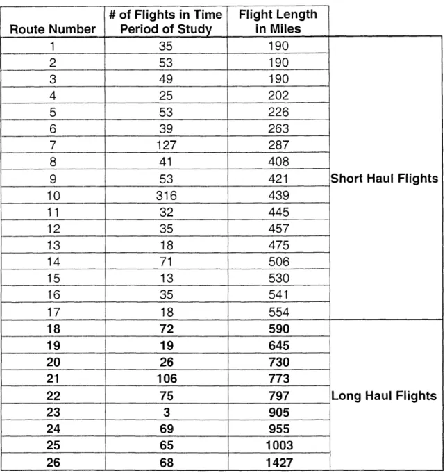
According to the criteria shown in table 2.2.2, we present all flights available to the study in table 2.2.3. Table 2.2.3 shows all the routes and flights available together with their frequency (total number of flights in time period) and the length of the flight. Table 2.2.3
classifies each route depending on the haul of the flight. It considers route number one the route with the shortest haul and route 26 the route with the longest haul.
Route Number 2 3 4 5 6 7 8 9 10 11 12 13 14 15 16 18 19 20 21 22 23 24 25 26 # of Flights in Time Period of Study 53 49 25 53 39 127 41 53 316 32 35 18 71 13 35 72 19 26 106 75 3 69 65 68 Flight Length in Miles 190 190 190 202 226 263 287 408 421 439 445 457 475 506 530 541 554 590 645 730 773 797 905 955 1003 1427
Short Haul Flights
Long Haul Flights
Table 2.2.3 / Classification of Flights According to their Haul.
The last variable to be considered is the day of the week in which the flight is
operated. We classify a day to be a Busy or Non-Busy day depending on the total number of domestic flights operated by the airline during that day. That number reflects demand for travel, and thus the number of passengers one might find on line at the ticket counter. Under this criterion, we are able to select the day with the highest number of flights as the busy day and the one with the lowest number of flights as the non-busy day. The results of applying these criteria were to select Thursday as the Busy day and Tuesday as the Non-Busy day as shown on table 2.2.4.
Busy Day Non- Busy Day
Thursday Tuesday
Table 2.2.4 / Busy and Non-Busy Day Selection.
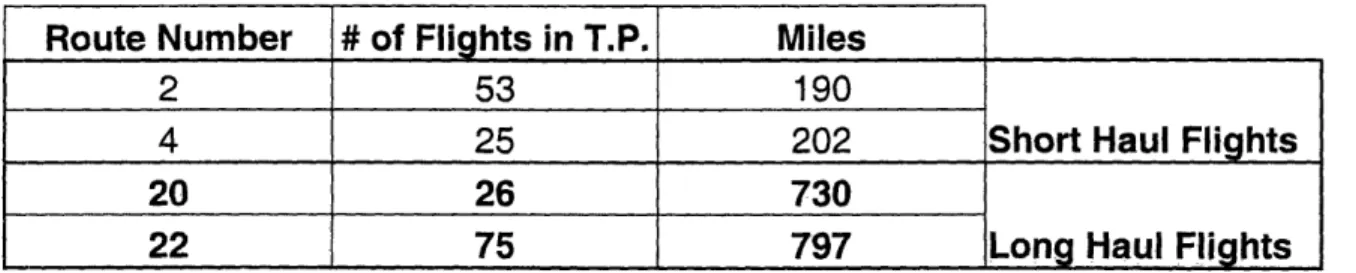
We illustrate the use of the Air Time metric by selecting four different routes from among the 26 routes available. These four routes have been selected in a way such that the mixture of leisure and business passengers can be assumed as equal in all of them. Table 2.2.5 summarizes the selected routes to be used.
# of Flights in T.P. 53 25 26 75 190 202 730 797
Short Haul Flights Long Haul Flights Table 2.2.5 / Routes to be Used in the Study Classified by Distance.
Miles Route Number 2 4 20 22
---j
For this first part of the analysis, we are interested in looking at the different
combination of the three variables affecting the passengers' arrival behavior and consequently the Air Time. As mentioned before, these elements are:
* Frequency * Distance
* Day of Week (Busy / Non-Busy)
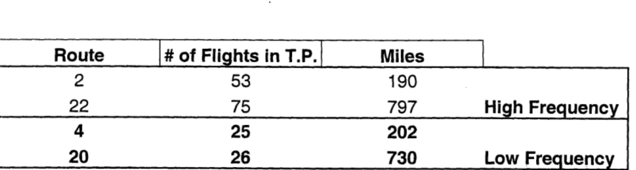
The selection of flights shown in table 2.2.5 defines six sets of flights. The first two sets, those corresponding to short / long haul flights are clearly indicated by the table. The sets corresponding to high / low frequency can be easily determined from the data on table 2.2.5 Therefore, we can also classify these four routes by flight frequency as shown in table 2.2.6. Finally, each of these flights will be analyzed on a busy and non-busy day making up for the last two sets to be considered.
Route # of Flights in T.P. Miles
2 53 190
22 75 797 High Frequency
4 25 202
20 26 730 Low Frequency
Table 2.2.6 / Routes to be Used in the Study Classified by Frequency.
We can verify the accuracy of the selection of the Busy / Non-Busy day by comparing the number of passengers handled by the airline on these days. To do this, for instance, we consider the passengers on Route 2 flying on Tuesdays and Thursdays on the different flights operated by the airline on those days. These data is presented on tables 2.2.7 and 2.2.8 for Tuesdays and Thursdays respectively.
Table 2.2.9 summarizes the results of tables 2.2.7 and 2.2.8 by comparing the total number of passengers carried by each flight number on Tuesdays and Thursday. As we will see along the study the selection of these days as the Busy and Non-Busy days will produce similar results in the other routes.
PAX
/
Flight #
Airplane
PAX on % of Capacity
Day
Flight
Date
Capacity Airplane
Used
Tuesday
307
17-Dec
142
54
38.0%
Total PAX
Tuesday
307
14-Jan
97
62
63.9%
Per Flight #
Tuesday
307
11-Feb
97
45
46.4%
161
Tuesday
315
17-Dec
142
79
55.6%
Total PAX
Tuesday
315
14-Jan
142
70
49.3%
Per Flight #
Tuesday
315
18-Mar
142
80
56.3%
229
Tuesday
405
17-Dec
97
68
70.1%
Total PAX
Tuesday
405
14-Jan
97
75
77.3%
Per Flight #
Tuesday
405
18-Mar
97
68
70.1%
211
Total
601
PAX
/
Month
Airplane
PAX on % of Capacity
Day
Flight
Date
Capacity Airplane
Used
Tuesday
307
17-Dec
142
54
38.0%
Total PAX
Tuesday
315
17-Dec
142
79
55.6%
Dec
Tuesday
405
17-Dec
97
68
70.1%
201
Tuesday
307
14-Jan
97
62
63.9%
Total PAX
Tuesday
315
14-Jan
142
70
49.3%
Jan
Tuesday
405
14-Jan
97
75
77.3%
207
Tuesday
307
11-Feb
97
45
46.4%
Total PAX
Tuesday
315
18-Mar
142
80
56.3%
Feb & Mar
Tuesday
405
18-Mar
97
68
70.1%
193
Total
601
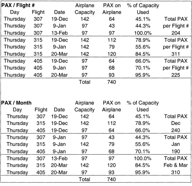
PAX / Flight # Airplane PAX on % of Capacity
Day Flight Date Capacity Airplane Used
Thursday 307 19-Dec 142 64 45.1% Total PAX
Thursday 307 9-Jan 97 43 44.3% per Flight #
Thursday 307 13-Feb 97 97 100.0% 204
Thursday 315 19-Dec 142 112 78.9% Total PAX
Thursday 315 9-Jan 142 79 55.6% per Flight #
Thursday 315 20-Mar 142 120 84.5% 311
Thursday 405 19-Dec 97 64 66.0% Total PAX
Thursday 405 9-Jan 97 68 70.1% per Flight #
Thursday 405 20-Mar 97 93 95.9% 225
Total 740
PAX / Month Airplane PAX on % of Capacity
Day Flight Date Capacity Airplane Used
Thursday 307 19-Dec 142 64 45.1% Total PAX
Thursday 315 19-Dec 142 112 78.9% Dec
Thursday 405 19-Dec 97 64 66.0% 240
Thursday 307 9-Jan 97 43 44.3% Total PAX
Thursday 315 9-Jan 142 79 55.6% Jan
Thursday 405 9-Jan 97 68 70.1% 190
Thursday 307 13-Feb 97 97 100.0% Total PAX
Thursday 315 20-Mar 142 120 84.5% Feb & Mar
Thursday 405 20-Mar 97 93 95.9% 310
Total 740
Table 2.2.8 / Total Number of Passenger Handled by the Airline on Thursdays / Route 2.
Tuesday Thursday
Flight PAX PAX
307 161 204
315 229 311
405 211 225
Total 601 740
Table 2.2.9 / PAX Handled on each Flight Number for ALL Flights Operated on the Busy / Non-Busy Days / Route 2.
With these three different variables -distance, frequency and day- we are able to form 8 possible triplets. In the next chapter, chapter 3, we analyze each of these triplets to
determine which combination of parameters affects the most the mean CF time of a flight. We conclude this section by presenting in table 2.2.10 a summary of the triplets and the routes associated with these variables that we will consider in our study.
Day
of Week
Frequency
Distance
Route
Non-Busy Day
High
Frequency
Short Haul
2
Busy Day
High
Frequency
Short Haul
2
Non-Busy Day
Low Frequency
Short Haul
4
Busy Day
Low Frequency
Short Haul
4
Non-Busy Day
High Frequency
Long Haul
22
Busy Day
High Frequency
Long Haul
22
Non-Busy
Day
Low Frequency
Long Haul
20
Busy Day
Low Frequency
Long Haul
20
3
Data Analysis I.
The analysis we will do in this chapter, is done by first taking for each route one flight on Tuesday and one flight on Thursday of the month of December. The days we will select for this purpose are Tuesday Dec. 17 th, 2002 and Thursday Dec. 19th, 2002 which as we
already saw comply with the definitions of Non-Busy and Busy days respectively.
This selection will generate eight different groups of flights to be studied, which correspond to each one of the triplets mentioned in table 2.2.10. Chapter 3 will, therefore, be divided in eight sections each one of them taking care of a particular triplet.
We will begin each section by first analyzing a particular flight in a given route in order to obtain the mean CF time and standard deviation of the arrival process of that flight and, if possible2, all the other quantities of interest associated with the Air Time metric.
Afterwards, we will take all3 available flights in the route operated either on all
Tuesdays or Thursdays in the time period of our study and calculate for each of these flights its mean CF time and standard deviation. We then average these results to present the mean values for both the Busy and Non-Busy days corresponding to each route.
2 The Airline only provided us with the information required to calculate the AP time and the FDD D for four
flights. Two of these flights correspond to Route 2 and the other two to Route 22. Out of these four flights, two were operated on Tuesday, Dec. 17th, 2002 and the other two on Thursday, Dec.
19t, 2002.
3 By all we mean all flights operated in either the busy or the non-busy days of the time period of our study (e.g. all flights operated on Tuesdays for Route 2 would be part of the analysis of the short-haul, high-frequency, non-busy day triplet).
3.1
Non-Busy
-
High Frequency
-
Short Haul Case.
For this first part of the analysis, we take Flight 315 / Route 2 operated on Tuesday Dec. 17th, 2002. According to our classification of flights given on tables 2.2.5 and 2.2.6 this
is a high frequency flight since this route has 53 flights in the time period considered and it is also a short haul flight with the destination airport at only 190 miles away from the airport of origin. Also, as stated on table 2.2.4 and verified on table 2.2.9, Tuesday is considered to be the Non-Busy day.
After processing the flight's history given by the airline, we are able to obtain the flight's arrival distribution function and consequently its mean CF time and standard deviation. These results are shown on table 3.1.1 and the complete CDF, PMF and 1-CDF functions are shown on table 3.1.2. We then present table 3.1.3 as a summary of the arrival process to the flight given in table 3.1.2.
Flight 315 Date 17-Dec
Dest. Route 2 Departs 955
Dist. 190 Freq. 53
Min 164 Mean 79.75
Max 18 Std 37.86
Table 3.1.1 / Summary of Results for Flight 315 / Dec. 17th, 2002.
These results show that on average, passengers flying on this flight arrived to the airline's check-in counter 79.75 minutes prior to the scheduled departure time of the flight at 9:55 AM. These results also show that the first passenger to check-in for the flight did so 164 minutes before the scheduled departure time and the last passenger to check-in did so only 18 minutes before SDT.
Minutes CDF 1-CDF PMF 164 0.019608 0.980392 0.019608 163 0.039216 0.960784 0.019608 158 0.058824 0.941176 0.019608 156 0.098039 0.901961 0.039216 152 0.117647 0.882353 0.019608 122 0.137255 0.862745 0.019608 116 0.156863 0.843137 0.019608 107 0.176471 0.823529 0.019608 104 0.196078 0.803922 0.019608 103 0.215686 0.784314 0.019608 98 0.235294 0.764706 0.019608 95 0.254902 0.745098 0.019608 94 0.294118 0.705882 0.039216 93 0.313725 0.686275 0.019608 86 0.333333 0.666667 0.019608 85 0.352941 0.647059 0.019608 84 0.411765 0.588235 0.058824 83 0.490196 0.509804 0.078431 82 0.509804 0.490196 0.019608 81 0.529412 0.470588 0.019608 80 0.54902 0.45098 0.019608 79 0.568627 0.431373 0.019608 72 0.607843 0.392157 0.039216 71 0.627451 0.372549 0.019608 68 0.647059 0.352941 0.019608 62 0.666667 0.333333 0.019608 54 0.686275 0.313725 0.019608 49 0.745098 0.254902 0.058824 48 0.764706 0.235294 0.019608 46 0.784314 0.215686 0.019608 42 0.823529 0.176471 0.039216 39 0.843137 0.156863 0.019608 38 0.901961 0.098039 0.058824 35 0.921569 0.078431 0.019608 34 0.941176 0.058824 0.019608 26 0.960784 0.039216 0.019608 25 0.980392 0.019608 0.019608 18 1 0 0.019608
Table 3.1.2 / Distribution Function for the Arrival Process of Passengers at the Counter Relative to the Scheduled Departure Time of Flight 315 / Dec. 1 7th,
Table 3.1.1, gives us then, the value of the mean CF time for Flight 315 / Route 2 operated on Tuesday Dec. 17th 2002 which is 79.75 minutes. In order to calculate the actual
Air Time for this flight, we need to know the AP time and the flight's departure delay (FDD) D. The first quantity, the AP time for this flight, can be easily read from table 3.1.4
% of
PAX
Minutes
Checked
151-180 11.76 121-150 1.96 91-120 17.65 61 - 90 35.29 31 -60 27.45 0 - 30 5.89Total
100.00
Table 3.1.3 / Summary of the Arrival Process for Flight 315 / Dec. 17th, 2002.
Table 3.1.4 has four different values given by the airline. The first value under the label of "OUT" is the time at which the plane left the gate, the push-out time. The second value under the label of "OFF" represents the time at which the plane took off from the departing airport.
Table 3.1.4 / Airplane's Operations Times.
Flight
315
Dest.
Route 2
Date
17-Dec Departs
955
Out
Off
On
In
1005
1020
1047
1050
Time from Scheduled Departure to Actual
Arrival at Destination Airport
55 Min.
The third value under the label of "ON" represents the actual time at which the plane landed at the destination airport, and finally, the value under the label of "IN" is the time at which the plane reached the gate at the destination airport and the passengers were allowed to leave the airplane.
From the information given in table 3.1.4, we determine the AP time as "Time IN" minus "Time OUT" or 10:50 minus 10:05 which gives us a value for the AP time of 45 minutes. We also get from this same table the data to calculate the flight's departure delay D which for this case is "Time OUT" minus SDT or 10:05 minus 9:55. Therefore, we have that D equals 10 minutes. The value of D that we get in the Air Time metric is in fact one of the
statistics generated by the DOT's on-time records.
This example shows as well that the "On-Time" metric and its different components are included in the Air Time and can be easily derived from it, and illustrates the limitations of considering the on-time records as the only statistics of flight performance while, on the other hand, shows the benefits of having a broader view of the travel process given by the Air Time metric.
With the values of the mean CF time, AP time and flight's departure delay (FDD) D, we calculate the average Air Time for this flight to be
E[Air Time] = 79.75 + 45 + 10
E[Air Time] = 134.75 minutes
Now that we have the Air Time, we proceed to calculate the other three quantities of interest - GF, PF, ATM and RFT.
GF = 0.6660
PF = 1 - GF = 0.3340
And for the ATM we have the relation ATM = E[Air Time] / Mi from which we get:
ATM = 134.75 / 190 = 0.7092
With this information we see that an average passenger who engaged in this flight spent 66.60% of his total travel time on the ground at the departing airport. This measure, however, is still a little bit misleading and the results can be even more dramatic because passengers can spend time in the plane while the plane is on the ground.
Therefore, if we really want to have an accurate understanding on how compares the time on which an average passenger actually flies - the time in which we really move from origin to destination - to the time he spends on ground either on the plane or in any other stage of the process, we calculate the Real Fly Time factor (RFT).
We defined the RFT factor as the Actual Flying Time (AFT) divided by the E[Air Time]. From table 3.1.4 we determine the AFT to be 27 minutes. This is the actual time the airplane was on the air (On Time - Off Time). Thus we calculate for this particular flight the RFT as:
RFT = AFT / E[Air Time]
RFT = 27 / 134.75
This means that an average passenger on this flight spent only 20.04% of the total time of his entire journey in actually moving himself from origin to destination. This type of
information provided by the Air Time metric could change the way people travel, particularly on short haul routes like this one. Suppose that is reasonable to assume that on average a person would spend the same time in going from his house to the airport than from his house to the highway which leads to the destination city and that the same is true for the destination city. Then for this particular case, driving from origin to destination (only on the highway) takes a person an average of 180 minutes -on this route the highway time is three hours-compared to the 134.75 required to travel by air.
Information like this, provided by the Air Time, could lead many people to think twice on how to go from one place to another, particularly when traveling to recreational places where it is common for families to go together and the price of saving 45 minutes on the highway can be rather high.
From this data we also see that the average time per mile was almost 0.71 minutes. It is interesting to note that if an airplane travels on average at 600 mi/hr then the minimum ATM we could obtain is 0.1 min / mi - provided the RFT is one.
This implies that the longer the flight the smaller the ATM a passenger will
experience. Therefore, if we consider the ATM as a measure of how efficiently is our time spent while traveling by air, we see that long haul flights are more time efficient than short haul flight. Therefore, the Air Time metric allows us to determine the time-efficiency of a flight which can be used to compare across different airlines.
We conclude this section with table 3.1.5 which includes all flights on Route 2 operated on Tuesdays during the time period considered. This table shows for each flight its mean CF time, standard deviation and Min/Max values of the arrival process distribution.
Table 3.1.5 also presents the average mean CF time obtained by averaging the mean CF times of all the flights operated on Tuesdays. Similar results are shown for the standard deviation and the Min / Max values of the arrival process distribution.
Dest Route 2
Tuesday
Flight
Date
Min
Max
Mean
Std
307 17-Dec 132 6 60.78 39.35 307 14-Jan 175 4 99.44 58.72 307 11-Feb 173 37 85.76 37.49 315 17-Dec 164 18 79.75 37.86 315 14-Jan 169 -1 87.16 47.65 315 18-Mar 145 21 69.95 29.47 405 17-Dec 150 8 69.13 40.52 405 14-Jan 135 29 86.38 27.82 405 18-Mar 119 18 74.89 28.22 Average 151.33 15.56 79.25 38.57
# of Flights
Month
Mean
3
17-Dec
69.88
3
14-Jan
91.00
1
11-Feb
85.76
2
18-Mar
72.42
3.2 Busy
-
High Frequency
-
Short Haul Case.
In this section, we again look at Flight 315 / Route 2. By our definitions, this is a high frequency flight since there are 53 flights in the time period considered and it is also
a short haul flight for which the destination airport is only 190 miles away from the departing airport. We focus our attention, though, on the flight operated on Thursday Dec 19t h 2002, which as we argued is the busy day.
After processing the flight's history given by the airline, we obtain the flight's arrival distribution function, mean CF time and standard deviation. These results are shown on table 3.2.1. Table 3.2.2 presents a summary of the arrival process to this flight.
Flight
315
Date
19-Dec
Dest.
Route 2 Departs
955
Dist.
190
Freq.
53
Min
167
Mean
72.18
Max
19
Std
37.63
Table 3.2.1 / Summary of Results for Flight 315 / Dec. 19th, 2002.
These results show that an average passenger on this flight arrived to the airline's check-in counter 72.18 minutes prior to the scheduled departure time of the flight at 9:55 AM. The first surprising result that we get in this study is that the mean CF time of a flight operated on the Busy day is shorter than the mean CF time of the same flight but operated on the Non-Busy day. So, for our short-haul / high frequency route we have 72.18 and 79.75 minutes for the mean CF times of the Busy and Non-Busy days respectively. These results are not an isolated case due to the particular selection of flights to be analyzed, but rather the tendency that we will observe all along our research.
This is an interesting an unexpected result given that one would think that on the Busy day the mean CF time of a flight should be larger than on the Non-Busy day. The reason of why this may happen could be better understood if the statistics of the queue to get to the check-in counters were available.
Nevertheless, we can speculate that the reason for this behavior may, in part, be caused by the airline itself. If we think that an average passenger does not really
distinguish what an airline would consider to be a Busy or Non-Busy day, then we could assume that the time at which passengers decide to arrive at the airport is independent of the Busy/Non-Busy factor. However, on the Busy days, when there are indeed more passengers traveling, arriving passengers to the airport find a larger queue to get to the check-in counters. If left alone, many of these passengers could not get to the counter on time for check in before the closing time of the flight. So it is common practice for airlines to call to the counter passengers when the flight is about to close which would yield a shorter mean CF time for the flight. However, as already said, this is pure speculation and verification is required.
In order to calculate the E[Air Time] for this flight, we need to know the AP time as well as the flight's departure delay D. The AP time for this flight can be easily read from table 3.2.3 % of PAX Minutes Checked 151 -180 9.23% 121- 150 1.54% 91-120 10.77% 61 - 90 38.46% 31 - 60 30.77% 0- 30 9.23% Total 100.00%
Table 3.2.3 has four different values given by the airline. The value under the label of "OUT" is the time at which the plane left the gat. The second value under the label of "OFF" represents the time at which the plane took off. The third value under the label of "ON" represents the actual time at which the plane landed at the destination airport and finally, the value under the label of "IN" is the time at which the plane reached the gate at destination airport and passengers were allowed to leave the plane.
Table 3.2.3 / Airplane's Operations Times.
From the information in table 3.2.3, we calculate the AP time as "Time IN" minus "Time OUT" or 10:50 - 9:55 which gives us a value for the AP time of 55 minutes. Notice that for this case, the flight's departure delay D has a value of zero which means that the flight left the gate on time at the SDT. With these values and the mean CF time we calculate the E[Air Time] for this flight as:
E[Air Time] = 72.18 + 55 + 0
E[Air Time] = 127.18 minutes
Now that we have the Air Time, we calculate the other quantities of interest associated with the Air Time metric - GF, PF, RFT and ATM.
Flight
315
Dest.
Route 2
Date
19-Dec
Departs
955
Out
Off
On
In
955
1010
1045
1050
Time from Scheduled Departure to Actual
Arrival at Destination Airport
55 Min.
GF = ( 72.18 + 0 )/ 127.18 = 0.5676
PF = 1 - GF = 0.4324
We get the ATM = E[Air Time] / Mi as:
ATM = 127.18 / 190 = 0.6694
With this information, we conclude that an average passenger on this flight spent almost 56.76% of his total travel time on ground at the departing airport. This quantity, as in the previous section, can be a little misleading because passengers can spend time in the plane while the plane is on the ground.
To see how the real flying time - the time in which we really move from origin to destination - compares to the Air Time, the total time of our journey which includes all different stages of this process including the real flying time, we calculate the Real Fly Time factor (RFT).
We again define the RFT factor as the Actual Fly Time (AFT) divided by the E[Air Time]. From table 3.2.3 we determine the AFT to be 35 minutes. This is the actual
time the airplane was on the air (On Time - Off Time). Thus we calculate that for this particular flight the RFT is:
RFT = AFT / E[Air Time]
RFT = 35 / 127.18 = 0.2752
Therefore, an average passenger on this flight spent only 27.52% of the total time of his journey in actually moving himself from origin to destination and the average time per mile was 0.6694 minutes compared to 0.7092 minutes of the previous subsection,
which means that in this flight the time of passengers was used a little bit more efficiently.
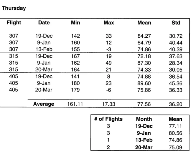
We end this section with table 3.2.4 which includes all flights on Route 2 operated on Thursdays during the time period considered. This table shows for each flight its mean CF time, standard deviation and Min/Max values of the arrival process distribution. Table 3.2.4 also presents the average mean CF time obtained by averaging the mean CF times of all the flights operated on Thursdays. Similar results are shown for the standard deviation and the Min / Max values of the arrival process distribution.
Dest Route 2
Thursday
Flight Date Min Max Mean Std
307 19-Dec 142 33 84.27 30.72 307 9-Jan 160 12 64.79 40.44 307 13-Feb 155 -3 74.86 40.39 315 19-Dec 167 19 72.18 37.63 315 9-Jan 162 49 87.30 28.34 315 20-Mar 164 21 74.33 30.05 405 19-Dec 141 8 74.88 36.54 405 9-Jan 180 23 89.60 45.36 405 20-Mar 179 -6 75.86 36.33 Average 161.11 17.33 77.56 36.20
# of Flights Month Mean
3 19-Dec 77.11
3 9-Jan 80.56
1 13-Feb 74.86
2 20-Mar 75.09
3.3 Non-Busy
-
Low Frequency
-
Short Haul Case.
We now turn our attention to the frequency factor and explore how low frequency affects the mean CF time of a flight. To illustrate this case, we consider Flight 353 / Route 4
operated on the non-busy day Tuesday Dec.17th 2002. This flight according to the definitions
given by tables 2.2.5 and 2.2.6 is a short haul flight with the destination airport at 202 miles from the airport of origin and it is also a low frequency flight with only 25 flights in the time period of our study.
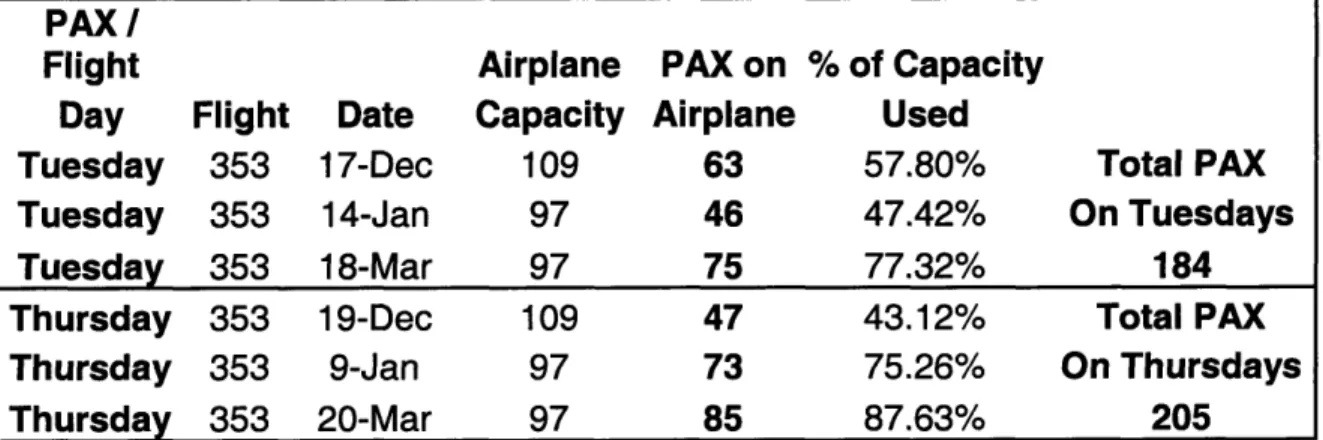
We present in table 3.3.1, the number of passengers handled on Route 4 on the Busy and Non-Busy days of our study. In this case, even though Flight 353 / Route 4 operated on Thursday Dec 19th 2002 carried less passenger than the one operated on Tuesday in the same
month, we still consider Tuesday as the Non-Busy day given that for all flights operated on Tuesdays and Thursdays in the route on the time period considered, more passengers were handled on Thursdays than on Tuesdays. Also, as said in section 2.2, we classified the Non-Busy / Non-Busy days by the total number of domestic flights operated by the airline and by the total number of passengers handled by the airline in the different days of the week and under these definitions Thursday still remains to be the Busy day.
PAX /
Flight Airplane PAX on % of Capacity
Day Flight Date Capacity Airplane Used
Tuesday 353 17-Dec 109 63 57.80% Total PAX
Tuesday 353 14-Jan 97 46 47.42% On Tuesdays
Tuesday 353 18-Mar 97 75 77.32% 184
Thursday 353 19-Dec 109 47 43.12% Total PAX
Thursday 353 9-Jan 97 73 75.26% On Thursdays
Thursday 353 20-Mar 97 85 87.63% 205
After analyzing the flight's history of Flight 353 / Route 4 operated on Tuesday Dec
17th 2002, we obtained the mean CF time and standard deviation of the arrival process
distribution. Table 3.3.2 presents a summary of these results and table 3.3.3 presents the summary of the arrival process to the flight.
Flight 353 Date 17-Dec
Dest. Route 4 Departs 1430
Dist. 202 Freq. 25
Min 150 Mean 106.72
Max 12 Std 31.68
Table 3.3.2 / Summary of Results for Flight 353 / Dec. 17th,2002.
% of PAX Minutes Checked 151 -180 0.00% 121-150 41.03% 91 - 120 25.64% 61 -90 25.64% 31-60 5.13% 0- 30 2.56% Total 100.00%
Table 3.3.3 / Summary of the Arrival Process for Flight 353 / Dec.17th, 2002.
From these results we see that an average passenger flying on this flight, arrived at the counter 106.72 minutes before the scheduled departure time of the flight at 14:30 Hrs - mean CF time. This reflects a significant increment in the mean CF time of the flight when compare to Flight 315 / Route 2 operated on the same date for which the mean CF time was 79.75
minutes. This result, which we will see all along our study, is the first indication we get that low frequency tends to increase the mean CF time of a flight.
For this flight, the airline did not provide us with the times at which the airplane left the gate, took off and arrived at the destination airport. For this reason we are unable to calculate the Air Time metric and the other statistics associated with it.
We conclude this section with table 3.3.4 which includes all flights on Route 4 operated on Tuesdays during the time period considered. This table shows for each flight its mean CF time, standard deviation and the times at which the first and last passenger checked-in.
Table 3.3.4 also presents the average mean CF time obtained by averaging the mean CF times of all the flights operated on Tuesdays. Similar results are shown for the standard deviation and the Min / Max values of the arrival process distribution.
If we compare the results of table 3.3.4 with those of table 3.1.5, we see that the average mean CF time for the low frequency flights is significantly higher than the average mean CF time for the high frequency flight - 94.17 compared to 79.25 respectively- showing the frequency effect on the mean CF time.
Dest Route 4
Tuesday
Flight
Date
Min
Max
Mean
Std
353 17-Dec 150 12 106.72 31.68
353 14-Jan 144 5 78.48 33.36
353 18-Mar 165 0 97.30 40.61
Average
153
5.67
94.17
35.22
3.4 Busy
-
Low Frequency
-
Short Haul Case.
We continue the analysis with Flight 353 / Route 4 operated on the busy day Thursday Dec. 19th 2002. This is a short haul, low frequency flight. The destination airport is 202 miles from the departing airport and the total number flights during the time period of our study is 25. After processing the flight's history, we obtained the statistics for this flight which include the mean CF time and standard deviation of the arrival distribution. Table 3.4.1 presents these results and table 3.4.2 presents the summary of the arrival process of passengers to the flight.
Flight
353
Date
19-Dec
Dest.
Route 4 Departs
1430
Dist.
202
Freq.
25
Min
126
Mean
58.06
Max
25
Std
28.47
Table 3.4.1 / Summary of Results for Flight 353 / Dec. 19th, 2002.
% of
PAX
Minutes
Checked
151-180 0.00% 121 -150 3.03% 91 - 120 9.09% 61 - 90 30.30% 31 - 60 36.36% 0 - 30 21.21%Total
100.00%
The result of this analysis shows a mean CF time for the flight of 58.06 minutes. This time is significantly smaller than the time we obtained in the previous subsection of 106.72 minutes for the Non-Busy day and it is actually one of the smallest we can find among the mean CF times of all the flights in the study. This result is congruent with our previous argument that on the busy day the mean CF time is smaller than on the non-busy day.
This result, however, differs from what it was expected. As seen in the previous sections, the higher the frequency the shorter the expected mean CF time of a flight.
Therefore, according to this general rule, which will be verified many times along the study, the flight operated on Route 2 on this same day should, on average, have a shorter mean CF time than this flight. We consider this result as an isolated case, non-representative of what in general occurs.
For this flight, as in the previous subsection, the airline did not provide us with the times at which the airplane left the gate, took off and arrived at the destination airport; reason for which we are unable to calculate the Air Time for this flight.
We end this section with table 3.4.3 which includes all flights on Route 4 operated on Thursdays during the time period considered. This table shows for each flight its mean CF time, standard deviation and Min/Max values of the arrival process distribution. Table 3.4.3 also presents the average mean CF time obtained by averaging the mean CF times of all the flights operated on Thursdays. Similar results are shown for the standard deviation and the Min / Max values of the arrival process distribution.
Dest Route 4
Thursday
Flight Date Min Max Mean Std
353 19-Dec 126 25 58.06 28.47
353 9-Jan 167 22 77.89 35.72
353 20-Mar 141 -7 70.38 35.12
Average 144.67 13.33 68.78 33.10