Reinforcement learning with raw image pixels as
input state
Damien Ernst†, Rapha¨el Mar´ee and Louis Wehenkel {ernst,maree,lwh}@montefiore.ulg.ac.be
Department of Electrical Engineering and Computer Science Institut Montefiore - University of Li`ege
Sart-Tilman B28 - B4000 Li`ege - Belgium
† Postdoctoral Researcher FNRS
Abstract. We report in this paper some positive simulation results ob-tained when image pixels are directly used as input state of a reinforce-ment learning algorithm. The reinforcereinforce-ment learning algorithm chosen to carry out the simulation is a batch-mode algorithm known as fitted Qiteration.
1
Introduction
Reinforcement learning (RL) is learning what to do, how to map states to ac-tions, from the information acquired from interaction with a system. In its clas-sical setting, the reinforcement learning agent wants to maximize a long term reward signal and the information acquired from interaction with the system is a set of samples, where each sample is composed of four elements: a state, the action taken while being in this state, the instantaneous reward observed and the successor state.
In many real-life problems, such as robot navigation ones, the state is made of visual percept. Up to now, the standard approach for dealing with visual percept in the reinforcement learning context is to extract from the images some relevant features and use them, rather than the raw image pixels, as input state for the RL algorithm (see e.g. [3]). The main advantage of this approach is that it leads to a reduction of the input space for the RL algorithm which eases the problem of generalization to unseen situations. Its main drawback is that the feature extraction phase needs to be adapted to problem specifics.
Recently, several research papers have shown that in the image classifica-tion framework, it was possible to obtain some excellent results by applying directly state-of-the-art supervised learning algorithms (e.g. tree-based ensem-ble methods, SVMs) on the image pixels (see e.g. [5]). Also, recent developments in reinforcement learning have led to some new algorithms which allow to take full advantage, in the reinforcement learning context, of the generalization per-formances of any supervised learning algorithm [1, 4]. We may therefore wonder whether using one of these new RL algorithms directly with the raw image pixels
as input state, without any feature extraction, could lead to some good perfor-mances. In a first attempt to answer this question, we carried out simulations and report in this paper our preliminary findings.
The next section of this paper is largely borrowed from [1] and introduces, in the deterministic case, the fitted Q iteration algorithm used in our simulations. Afterwards, we describe the test problem and discuss the results obtained in various settings. And, finally, we conclude.
2
Learning from a set of samples
2.1 Problem formulation
Let us consider a system having a deterministic discrete-time dynamics described by:
xt+1 = f (xt, ut) t = 0, 1, . . . (1)
where for all t, the state xtis an element of the state space X, the action utis
an element of the action space U .
To the transition from t to t + 1 is associated an instantaneous reward signal rt = r(xt, ut) where r(x, u) is the reward function bounded by some constant
Br.
Let µ(·) : X → U denote a stationary control policy and Jµdenote the return
obtained over an infinite time horizon when the system is controlled using this policy (i.e. when ut = µ(xt), ∀t). For a given initial condition x0 = x, Jµ is
defined as follows: Jµ(x) = lim N →∞ N −1X t=0 γtr(x t, µ(xt)) (2)
where γ is a discount factor (0 ≤ γ < 1) that weighs short-term rewards more than long-term ones. Our objective is to find an optimal stationary policy µ∗,
i.e. a stationary policy that maximizes Jµ for all x.
Reinforcement learning techniques do not assume that the system dynamics and the cost function are given in analytical (or even algorithmic) form. The sole information they assume available about the system dynamics and the cost function is the one that can be gathered from the observation of system trajec-tories. Reinforcement learning techniques compute from this an approximation ˆ
π∗
c,T of a T -stage optimal (closed-loop) policy since, except for very special
con-ditions, the exact optimal policy can not be decided from such a limited amount of information.
The fitted Q iteration algorithm on which we focus in this paper, actually relies on a slightly weaker assumption, namely that a set of one step system transitions is given, each one providing the knowledge of a new sample of in-formation (xt, ut, ct, xt+1) that we name four-tuple. We denote by F the set
{(xl
t, ult, clt, xlt+1)} #F
2.2 Dynamic programming results
The sequence of QN-functions defined on X × U
QN(x, u) = r(x, u) + γmax
u′∈UQN −1(f (x, u), u
′)∀N > 0
with Q0(x, u) ≡ 0 converges, in infinity norm, to the Q-function, defined as the
(unique) solution of the Bellman equation: Q(x, u) = r(x, u) + γmax
u′∈UQ(f (x, u), u
′) (3)
A policy µ∗ that satisfies
µ∗(x) = arg max u∈U
Q(x, u) (4)
is an optimal stationary policy. Let us denote by µ∗
N the stationary policy
µ∗
N(x) = arg max u∈U
QN(x, u) . (5)
The following bound on the suboptimality of µ∗ N holds: kJµ∗ − Jµ∗ Nk ∞≤ 2γNB r (1 − γ)2 . (6) 2.3 Fitted Q iteration
The fitted Q iteration algorithm computes from the set of four-tuples F the func-tions ˆQ1, ˆQ2, . . ., ˆQN, approximations of the functions Q1, Q2, . . ., QN defined
by Eqn (3), by solving a sequence of standard supervised learning regression problems. The policy
ˆ
µ∗N(x) = arg max u∈U
ˆ
QN(x, u) (7)
is taken as approximation of the optimal stationary policy. The training sample for the kth problem (k ≥ 1) of the sequence is
((xl
t, ult), rtl+ γmax u∈U
ˆ
Qk−1(xlt+1, u)), l = 1, . . . , #F (8)
with ˆQ0(x, u) = 0 everywhere. The supervised learning regression algorithm
produces from this training sample the function ˆQk that is used to determine
pt 0 0 20 100 100 p(0) p(1) pt+1(1) = min(pt(1) + 25, 100) possible actions r(p, u) = 2 r(p, u) = 0 r(p, u) = 1 20 ut= go up 0 0 20 100 100 p(0) p(1) 20 (a) (b)
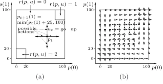
Fig. 1.Figure (a) gives information for the position dynamics and the reward function for the agent navigation problem. Figure (b) plots the optimal policy µ∗(p) for the values of p ∈ {0, 10, . . . , 100}×{0, 10, . . . , 100}. Orientation of the triangle for a position pgives information about the optimal action(s) µ∗(p).
3
Simulation results
3.1 The test problem
Experiments are carried out on the navigation problem whose main characteris-tics are illustrated on Figure 1a. An agent navigates in a square and the reward he gets is function of his position in the square. He can at each instant t either decide to go up, down, left of right (U = {up, down, lef t, right}). We denote by p the position of the agent. The horizontal (vertical) position of the agent p(0) (p(1)) can vary between 0 and 100 with a step of 1. The set of possible positions is P = {0, 1, 2, . . . , 100} × {0, 1, 2, . . . , 100}. When the agent decides at time t to go in a specific direction, he moves 25 steps at once in this direction, unless he is stopped before by the square boundary.
The reward signal rtobserved by the agent is always zero, except if the agent
is at time t in the upper right part of the square and the lower left part of the square where reward signals of 1 and 2 are observed, respectively (Br= 2). The
decay factor γ is equal to 0.5. The optimal policy, plotted on Figure 1b drives the agent to one of these corners. Even if larger reward signals are observed the lower left corner, the optimal policy does not necessarily drive the system to this corner. Indeed, due to the discount factor γ that weighs short-term reward signal more than long-term ones, it may be preferable to observe smaller reward signals but sooner.
Our goal is to study the performances of the fitted Q iteration algorithm when the input state for the RL algorithm is not the position p but well a visual percept. In this context, we represent on top of the navigation square a navigation image, and we have supposed that when being at position p, the agent has access to the visual percept pixels(p) which is a vector of pixel values that encodes the image region surrounding its position p (Figure 2). The matrix giving the grey levels of the 100 tiles of Figure 2 is given in 5.
0 0 100 100 p(0) p(1) pt 10 pixels pt 15 pixels 100 pixels 30 pixels
the agent is in positon pt
is the (30 ∗ i + j)th element of this vector. the grey level of the pixel located at the ith line grey level∈ {0, 1, · · · , 255}
pixels(pt) = 30*30 element vector such that
pixels(pt)
and the jth column of the observation image observation imagewhen
186 186103 103 250 250 250 250
Fig. 2.Visual percept pixels(pt) for the agent when being position pt. Pixels of the
30 × 30 observation image which are not contained in the 100 × 100 navigation image, which happens when pt(i) < 15 and/or pt(i) > 85, are assumed to be black pixels (grey
level=0).
In our study, we have partionned the 100 × 100 navigation image into one hundred 10 × 10 subimages that we name tiles. For every tile, we have selected a grey level at random in {0, 1, . . . , 255} and set all its pixels to this grey level. After having generated the image, we have checked whether two different positions p were indeed leading to different vectors of pixel values pixels(p). This check has been done in order to make sure that considering pixels(p) rather than p as input state does not lead to a partially observable system.
3.2 Four-tuples generation
To generate the four-tuples we consider one step episodes with the initial position for each episode being chosen at random among the 101 ∗ 101 possible positions p and the action being chosen at random among U . More precisely, to generate a set F with n elements, we repeat n times the sequence of instructions: 1. draw p0 at random in P and u at random in U ;
2. observe r0 and p1;
3. add (pixels(p0), u0, r0, pixels(p1)) to F .
3.3 Fitted Q iteration algorithm
Within the fitted Q iteration algorithm, we have used in our simulations a regres-sion tree based ensemble method called Extra-Trees [2].1To apply this algorithm
at each iteration, the training sample defined by Eqn (8) is split into four subsam-ples according to the four possible values of u, and ˆQk(x, u) for each value of u is
obtained by calling the Extra-Trees algorithm on the corresponding subsample.
1 The Extra-Trees algorithm has three parameters M (the number of trees that are
built to define the ensemble model), nmin (the minimum number of samples of
non-terminal nodes) and K (the number of cut-directions explored to split a node). They have been set to M = 50, nmin = 2 (yielding fully developed trees) and K = 900
0 0 100 100 p(0) p(1) 0 0 100 100 p(0) p(1)
(a) ˆµ∗10, 500 four-tuples (b) ˆµ∗10, 2000 four-tuples
0 0 100 100 p(0) p(1) 1000 5000 7000 9000 0.4 0.6 0.8 3000 1.
pused as state input Optimal score (Jµ∗)
#F Jµˆ
∗ 10
pixels(p) used as state input
(c) ˆµ∗10, 8000 four-tuples (d) score versus nb four-tuples
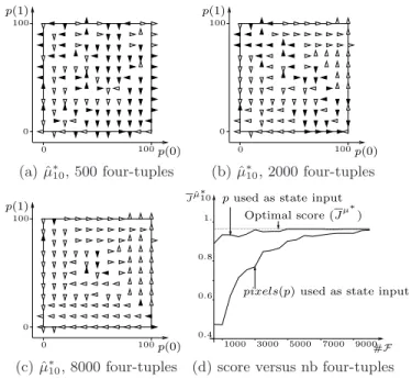
Fig. 3.Figures (a-c) plot the policy ˆµ∗10 computed for increasing values of #F . The
orientation of the triangles indicate the value of ˆµ∗10(pixels(p)); white triangles indicate
that it coincides with an optimal action. Figure (d) plots the score of the policies: the horizontal line indicates the score of the optimal policy, the darker curve (with smaller scores) corresponds to the case of pixel based learning with growing number of four-tuples, while the lighter curve provides the scores obtained with the same samples when the position p is used as state representation.
The number of iterations N of the fitted Q iteration algorithm is chosen equal to 10, leading to an upper bound of 0.015625 in Eqn (6) which is tight enough for our purpose, since Jµ∗
(x) ∈ [0.25, 4]. The policy ˆµ∗
10(x) = arg maxuQˆ10(x, u)
is taken as approximation of the optimal stationary policy.
3.4 Results
Figures 3a-c show how the policies ˆµ∗
10 change when increasing the size of the
set of four-tuples. In particular, Figure 3c shows that with 8000 four-tuples, the policy almost completely coincides with the optimal policy µ∗ of Figure 1b. To
further assess the speed of convergence of the algorithm, we have plotted on Figure 3d the score2of policies obtained in different conditions. We observe that
with respect to the compact state representation in terms of positions, the use
2 The score of a policy is defined here as the average value over all possible initial
states of the return obtained over an infinite time horizon when the system follows this policy.
Jµˆ ∗ 10 1. 0.4 0.6 0.8 Optimal score (Jµ∗) 100×100 10×10 20×20 50×50 5×5
System partially observable 1×1
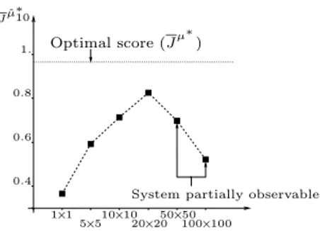
Fig. 4.Evolution of the score with the size of the constant grey level tiles. #F = 2000.
of the pixel based representation slows down but does not prevent convergence. Indeed, with #F = 10, 000 the score of the pixel based policy has almost con-verged to the optimal one, which is a fairly small sample size if we compare it to the dimensionality of the input space of 900. This suggests that the fitted Q iteration algorithm coupled with Extra-Trees is able to cope with a low-level representation where information is scattered in a rather complex way over a large number of input variables.
To illustrate the influence of the navigation image characteristics on the results, we carried out an experiment where we have changed the size of the constant grey level tiles while keeping constant the size of the observation images. The results, depicted on Figure 4, show that the score first increases, reaches a maximum, and decreases afterwards.
To explain these results, we first notice that the Extra-Trees method works by inferring from a sample T S = ((il, ol), l = 1, . . . , #T S) a kernel K(i, i′), from
which an approximation of the output o associated with an input i is computed by ˆo(i) =P(il,ol)K(i, il)ol. The value of K(i, il) thus determines the importance
of the output ol in the prediction, and for our concern the main property of the
Extra-Trees kernel is that it takes larger values if the vectors i and il have
many components which are close to each other, i.e. if there exists many values of j ∈ {1, 2, · · · , size of vector i} such that i[j] is close from il[j] [2]. Next, we
note from Figure 3d that when the algorithm is applied to a training set of size 2000 with positions as inputs (i.e. T Sp= ((pl, ol), l = 1, . . . , #T Sp)) it provides
close to optimal scores. With this input representation, elements (pl, ol) such
that pl is geometrically close to p tend to lead to a high value of K(p, pl) and
one may therefore reasonably suppose that when using pixel vectors as inputs, good results will be obtained only if the resulting kernel K(pixels(p), pixels(pl))
is strongly enough correlated with the geometrical distance between p and pl,
which means that the closer two positions the more similar the corresponding vectors of pixel values should be.
With this we can explain the influence of the size of the tiles on the score in the following way. Let pl be a position such that its 30 × 30 observation image
is fully contained in the square. Then, when the navigation image is composed of randomly chosen 1 × 1 tiles, for a position p 6= pl there is no reason that
the value of K(pixels(p), pixels(pl)) should depend on the geometrical distance
between p and pl. In other words, the kernel derived in these conditions will
take essentially only two values, namely K(pixels(p), pixels(pl)) = 1 if p = pl
and K(pixels(p), pixels(pl)) ≈ 1/#T S otherwise. Thus, the output predicted at
a position far enough from the square boundary will essentially be the average output of the training set, except for positions contained in the training sample. When the tiles become larger, the dependence of the amount of similar pixels of two observation images on their geometrical distance increases, which leads to a more appropriate approximation architecture and better policies. However, when the tiles size becomes too large the sensitivity of the pixel based kernel with respect to the geometrical distance eventually decreases. In particular, the loss of observability above a certain tiles size translates into a dead-band within which the kernel remains constant, which implies suboptimality of the inferred policy, even in asymptotic conditions.
4
Conclusions
We have applied in this paper a reinforcement learning algorithm known as fit-ted Q iteration to a problem of navigation from visual percepts. The algorithm uses directly as state input the raw pixel values. The simulation results show that in spite of the fact that in these conditions the information is spread in a rather complex way over a large number of low-level input variables, the rein-forcement learning algorithm was nevertheless able to converge relatively fast to near optimal navigation policies. We have also highlighted the strong depen-dence of the learning quality on the characteristics of the images the agent gets as input states, and in particular on the relation between distances in the high-dimensional pixel-based representation space and geometrical distances related to the physics of the navigation problem.
5
Image description
We provide hereafter the 10 × 10 matrix giving the grey levels of the 100 tiles of Figure 2: 2 6 6 6 6 6 6 6 6 6 6 6 6 6 6 4 164 55 175 6 132 27 35 255 47 11 169 155 87 5 77 39 197 179 82 111 5 92 176 10 148 37 57 119 32 193 156 110 54 38 186 103 190 212 241 108 65 103 125 239 73 235 128 199 3 247 42 129 233 3 250 101 196 119 108 192 199 91 240 254 71 2 250 250 36 227 109 150 111 224 244 152 57 205 173 174 124 242 42 62 0 234 252 127 28 114 163 7 198 92 192 163 115 208 160 168 3 7 7 7 7 7 7 7 7 7 7 7 7 7 7 5
References
1. D. Ernst, P. Geurts, and L. Wehenkel. Tree-based batch mode reinforcement learn-ing. Journal of Machine Learning Research, 6:503–556, April 2005.
2. P. Geurts, D. Ernst, and L. Wehenkel. Extremely randomized trees. Machine Learning, 36(1):3–42, 2006.
3. S. Jodogne and J. Piater. Interactive learning of mappings from visual percepts to actions. In L. De Raedt and S. Wrobel, editors, Proceedings of the 22nd International Conference on Machine Learning, pages 393–400, August 2005.
4. M. Lagoudakis and R. Parr. Reinforcement learning as classification: leveraging modern classifiers. In T. Faucett and N. Mishra, editors, Proceedings of 20th Inter-national Conference on Machine Learning, pages 424–431, 2003.
5. R. Mar´ee, P. Geurts, J. Piater, and L. Wehenkel. Random subwindows for robust image classification. In C. Schmid, S. Soatto, and C. Tomasi, editors, Proceedings of the IEEE International Conference on Computer Vision and Pattern Recognition, volume 1, pages 34–40. IEEE, June 2005.