wide association studies by random forests
Vincent Botta1,3, Sarah Hansoul2,3, Pierre Geurts1,3, and Louis Wehenkel1,3
1
Department of Electrical Engineering and Computer Science 2
Animal Genomics
3 GIGA-Research, University of Li`ege, B4000 Belgium
Abstract. We consider two different representations of the input data for genome-wide association studies using random forests, namely raw genotypes described by a few thousand to a few hundred thousand dis-crete variables each one describing a single nucleotide polymorphism, and haplotype block contents, represented by the combinations of about 10 to 100 adjacent and correlated genotypes. We adapt random forests to exploit haplotype blocks, and compare this with the use of raw geno-types, in terms of predictive power and localization of causal mutations, by using simulated datasets with one or two interacting effects.
Key words: Random forests, genome-wide association studies, complex diseases, variable importance measures
1
Introduction
The majority of important medical disorders (f.i. susceptibility to cancer, cardio-vascular diseases, diabetes, Crohn’s disease) are said to be complex. This means that these diseases are influenced by multiple, possibly interacting environmen-tal and genetic risk factors. The fact that individuals differ in terms of exposure to environmental as well as genetic factors explains the observed inter-individual variation in disease outcome (i.e. phenotype). The proportion of the phenotypic variance that is due to genetic factors (heritability) typically ranges from less than 10 to over 60 % for the traits of interest. The identification of genes influenc-ing susceptibility to complex traits reveals novel targets for drug development, and allows for the implementation of strategies towards personalized medicine.
Recent advances in marker genotyping technology allow for the genotyping of hundreds of thousands of Single Nucleotide Polymorphisms (SNP) per individual at less than 0.1 eurocents per genotype. The identification of genomic regions (i.e. loci) that influence susceptibility to a given disease can now be obtained by means of so-called “genome-wide association studies” (GWAS). Basically, the idea behind GWAS of complex diseases is to genotype a collection of affected (cases) and unaffected (controls) individuals for a very large number of genetic markers spread over the entire genome. Typically, one disposes of a cohort of a few hundred to a few thousand individuals, a fraction of them (typically about 50%) having a certain phenotype (e.g. disease status, or treatment response
status), and the rest of them being controls (individuals representative of the genetic variation in the studied population and who do not present the stud-ied phenotype). In this domain, supervised learning, and in particular Random Forests, has been recently proposed to circumvent the limitations of standard approaches based on univariate statistical tests [1–3].
In this paper, we study two different representations of the input data for the application of supervised learning in GWAS, namely the raw SNP genotypes on the one hand, and on the other hand new features derived from groups of strongly correlated SNPs (i.e. the haplotype blocks; those blocks are transmitted from parents to offspring during the recombination of parental chromosomes). We propose an adaptation of Random Forests to handle haplotype blocks as well as SNPs. Currently, available real-life datasets are still being investigated by the geneticists, for this reason, as a first step, we compare the two approaches empirically on simulated datasets with one or two independent or interacting causal mutations. Our two contributions with respect to previous work are the exploitation of haplotype blocks and its systematic evaluation on high density simulated datasets, both for genetic risk assessment and for the localization of causal mutations.
The rest of the paper is organized as follows. In Section 2, we describe the al-gorithms, while Section 3 presents the simulated datasets and simulation results. We conclude in Section 4 with discussions and future work directions.
2
Methods and algorithms
2.1 Random forests
From a machine learning point of view, a GWAS of a complex disease is a binary classification problem, with a very large number of raw variables, each one corresponding to a different SNP and having only three possible values (homozygous wild, heterozygous and homozygous mutant). On top of this very high p/n ratio, these problems are also generally highly noisy, and the raw input variables are strongly correlated (due to linkage disequilibrium).
The nature of the problem puts several constraints on candidate supervised learning methods. The method needs to find a small number of relevant variables among a very large number of irrelevant ones, and thus incorporate some feature selection mechanism. It needs to be sufficiently expressive to take into account possible interactions between SNPs. Computationally, the algorithm should fur-thermore be able to cope with hundreds of thousands of variables and thousands of individuals. Tree-based ensemble methods provide a good tradeoff along these criteria. Among existing ensemble methods, we focus in this paper on the Ran-dom Forests algorithm [4]. This algorithm grows each tree of the ensemble from a bootstrap sample drawn from the original data, using the CART algorithm (without pruning) with a modified node splitting procedure. At each test node, the algorithm selects the best split using the standard CART procedure but from a subset of only K attributes selected at random among all candidate attributes.
2110 1121 2020 12000 00222 00222 20 12 22
block1 block2 block3 . . . 2 1 1 0 1 2 0 0 0 2 0 1 1 2 1 0 0 2 2 2 1 2 2 0 2 0 0 0 2 2 2 2 2 snp1snp2 snp11 . . . Hotspots
SNP representation Block representation
Fig. 1. Database transformation from SNPs to haplotype blocks.
The algorithm performances depend on the number T of trees in the ensemble (the larger the better) and on the number K of selected attributes at each test node, whose optimal value is problem dependent.
2.2 Individual SNP and haplotype block representations
Figure 1 shows the two representations of input data that we will use for growing Random Forests, and how the block contents are computed from the SNPs. SNPs are arranged as they appear along the chromosome and the integer values {0, 1, 2} represent the number of mutant alleles at the corresponding position.
In order to apply Random Forests on the raw genotype data, we merely consider each SNP as a numerical variable. To handle attributes representing the contents of haplotype blocks, we propose the following adaptation of the node-splitting procedure:
– At each test-node, K blocks are selected at random. – For each block b, we proceed as follows:
• for each SNP i in b, we compute from the subset of cases (resp. controls) at the test-node the frequency of its three possible values (fb
i,j)case(resp.
(fb
i,j)control) (i = 1, . . . , lb, j = 0, 1, 2), where lb denotes the number of
SNPs in b;
• for each case or control x, we compute the two probabilities :
P (x|case, b, node) = lb Y i=1 (fj,sb i(b,x))case (1) and P (x|control, b, node) = lb Y i=1 (fj,sb i(b,x))control, (2)
where si(b, x) denotes the value of the ith SNP of b for this individual
x;4
4
This is a maximum likelihood based estimation of the conditional probability that the observed haplotype is drawn from the population of cases (resp. controls) reaching the current node, assuming class conditional independance of the SNPs in the block b.
• then, an optimal cutoff is determined on the probability ratio: P (x|case, b, node)
P (x|control, b, node) (3)
using the standard CART procedure for numerical variables. – The best split among the K optimal splits is selected to split the node.
Notice that the motivation behind the block-wise approach is to reduce the number of features by grouping correlated SNPs, and thus to improve the ro-bustness of the method. In our description, we left open the question of the de-termination of the blocks. In our experiments, we will compare two approaches. First, haplotype blocks delimited by HapMap hotspot list generated from a panel of 5 populations from which our simulated data will be derived, second, haplo-type blocks reconstructed from a linkage disequilibrium map computed by the Haploview software [5] applied on our simulated datasets.
2.3 Localization of causal mutations
Several importance measures have been proposed in the literature to derive from a tree ensemble a ranking of candidate attributes according to their relevance for predicting the output. In the context of GWAS, such measures may be used to identify the SNPs or haplotype blocks closest to the causal mutation loci. In our simulations we use to this end the information theoretic measure proposed in [6] computing for each attribute the total reduction of class entropy (the sum over all test-nodes of the ensemble where this attribute is used, of the local reduction in entropy weighted by the local sample size).
3
Experiments
3.1 Simulated dataset
We used gs [7] to generate samples based on HapMap data [8] with linkage disequilibrium patterns similar to those in actual human populations. We focus our experiments on chromosome 5 (because its size is close to the mean size of other human chromosomes). The raw input variables were obtained by taking SNPs spaced by 10 kilobases from the HapMap pool to reproduce classical GWAS conditions, and the causal disease loci were removed from the input variables.
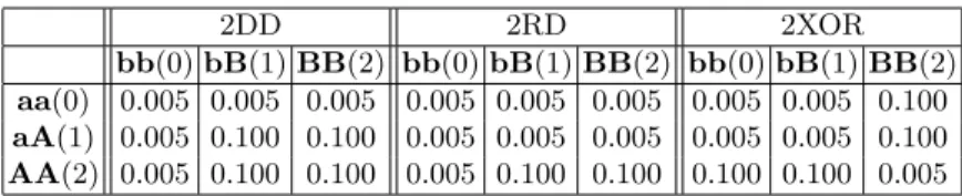
Five different disease models were tested: two models with one disease locus, and three models with two interacting loci. Tables 1 and 2 give the penetrance matrix for each model. These tables report the probabilities of being affected for each possible genotype of the locus or loci. Lower case letters (a, b) denote wild alleles and upper case letters (A, B) denote mutant alleles. We introduce a noise level of 0.005 to simulate environmental effects. The 3 two loci models were selected among the most common disease models referenced in [9].
Table 1. The one-locus disease models that were investigated in this study.
1A 1aA
aa(0) aA(1) AA(2) aa(0) aA(1) AA(2)
0.005 0.005 0.100 0.005 0.100 0.250
Table 2. The two-locus disease models that were investigated in this study.
2DD 2RD 2XOR
bb(0) bB(1) BB(2) bb(0) bB(1) BB(2) bb(0) bB(1) BB(2)
aa(0) 0.005 0.005 0.005 0.005 0.005 0.005 0.005 0.005 0.100
aA(1) 0.005 0.100 0.100 0.005 0.005 0.005 0.005 0.005 0.100
AA(2) 0.005 0.100 0.100 0.005 0.100 0.100 0.100 0.100 0.005
The first two disease models (Table 1) contain one susceptibility locus. In the first one, 1A, two copies of the mutant allele increase the risk of being affected. The second one 1aA is additive: the risk increases with the number of mutant alleles present at the susceptibility locus. The three disease models described in Table 2 involve two susceptibility loci. For the 2DD model (dominant-dominant), the two loci are dominant, meaning that at least one copy of the mutant allele at the two loci is required for the risk to increase. The 2RD model (recessive-dominant) requires two copies of disease alleles from the first locus and at least one disease allele from the second. Finally, in the 2XOR model, two mutant copies at one locus or three mutant copies at any of them increase the disease risk.
In the first (raw) data representation, the different databases are composed of about 14000 numerical variables. This number was reduced to 2000 variables of HapMap blocks and 6500 variables of blocks obtained with Haploview.
3.2 Protocol
For each disease model, we generated 7000 individuals (with 50% of cases) that we divided into 2000 individuals for learning and 5000 individuals for testing. The learning sample was divided into 4 subsets of size 500. A model was produced for each subset of size 500. We report average results (and standard deviations) over all subsets.
The predictive power was assessed using the area under the ROC curves (AUC) computed on the 5000 test samples and averaged over the training set and compared to the AUC obtained on the test samples with the Bayes optimal model deduced directly from the selected disease model. The latter is denoted as “Ref AUC” in the tables and figures reported below.
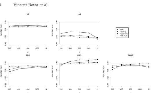
K AUC/REF AUC 1A 200 400 800 1600 N 0.94 0.96 0.98 1.00 ● ● ● ● ● K AUC/REF AUC 1aA 200 400 800 1600 N 0.94 0.96 0.98 1.00 ● ● ● ● ● K AUC/REF AUC 2DD 200 400 800 1600 N 0.94 0.96 0.98 1.00 ● ● ● ● ● K AUC/REF AUC 2RD 200 400 800 1600 N 0.94 0.96 0.98 1.00 ● ● ● ● ● K AUC/REF AUC 2XOR 200 400 800 1600 N 0.94 0.96 0.98 1.00 ● ● ● ● ● ● ● ● SNP HapMap Haploview REF AUC
Fig. 2. Influence of parameter K on the five disease models. In plain: SNP; in dotted:
HapMap; in dashed: Haploview ; in gray: the ratioREF AU CAU C . N denotes the total number
of candidate attributes for each type of representation.
3.3 Empirical results
Parameter sensitivity. We first carried out some preliminary experiments to see the effect of the two parameters of the Random Forests algorithm. Given the important number of attributes, we observed that a quite large number of trees is necessary for the error to converge. In all our experiments, we therefore conservatively fixed T to 2000 trees. We also observed that small values of K (< 200) yield to suboptimal AUC values, and we therefore only explored higher values of K.
Figure 2 shows the evolution of the AUC for the five disease models with the K parameter and all three approaches (RF with raw SNPs, HapMap and Haploview blocks). Note that in this graph, N is very different from one method to another (resp. 14000, 2000, and 6500 for SNP, HapMap and Haploview ). We observe that HapMap and Haploview produce slightly better results than SNPs for the models 1A, 2DD, 2RD, and 2XOR. Typically, larger values of K yield very close to optimal results. Note however that the maximal AUC is usually already obtained with significantly lower values of K (1600), which correspond also to smaller computational requirements. In our experiments below, we will thus present only the results for this setting.
Table 3. AUC (average ± std. dev.) for K=1600.
SNP HapMap Haploview Ref AUC
1A 0.7311 ± 0.0048 0.7296 ± 0.0061 0.7315 ± 0.0048 0.7386
1aA 0.7901 ± 0.0016 0.7800 ± 0.0025 0.7820 ± 0.0020 0.8142
2DD 0.8112 ± 0.0012 0.8131 ± 0.0012 0.8124 ± 0.0011 0.8198
2RD 0.6377 ± 0.0072 0.6358 ± 0.0044 0.6403 ± 0.0033 0.6354
2XOR 0.7927 ± 0.0037 0.7969 ± 0.0040 0.7944 ± 0.0012 0.7984
Predictive power. Table 3 reports AUCs for the different methods for all considered disease models with K = 1600. Overall, the results of the SNP rep-resentation and the two types of blocks are very close to each other and to the “Ref AUC” on most of the models. Blocks outperform the SNPs on 1A, 2DD, 2RD and 2XOR. The HapMap blocks outperform the Haploview on 1A, 2DD and 2XOR.
Localisation of causal mutations. For the one locus model the causal mu-tation (A) is located at position 1599; for the two-loci model the first causal mutation (A) is located also at position 1599, while the second one (B) is lo-cated far away, at position 11175. Figure 3 shows the SNP importances over the chromosome 5, while Figure 4 provides a zoom of the variable importances of the three methods over the regions close to the two causal loci of the two-loci disease models. We observe that in all cases, except for 2RD, the genomic regions containing the two causal mutations are very well localized.
4
Conclusions
The preliminary results obtained in this paper show promising perspectives. In particular, the different methods obtain rather good AUCs as compared with the theoretical upper bound derived from the disease models. The different methods are also able to predict and to localize the disease loci, rather well. We observed that most often our adaptation of Random Forests to the block representation of the data provides marginally superior results in terms of risk prediction than their direct application to the raw genotype data. Results not reported in this paper with different ensembles of trees do not contradict these findings.
An interesting direction of future research will be the refinement of the treate-ment of the haplotype block structure in supervised learning. In the context of tree-based methods, we envisage two extensions of the splitting procedure: first, there are various possible ways to improve the way likelihoods are computed within a block, e.g. by relaxing class-conditional independance; second, one could use overlapping (and of randomized length) block structures or greedily search for optimal block size around a SNP of interest locally at each tree node, instead of exploiting an a priori fixed block structure. More generally, we believe that the simultaneous exploitation of blocks and SNPs may also be of interest.
Future work will also consider more complex disease models, real-life datasets, quantitative traits, as well as even higher density genotyping, in the limit towards the next generation of full genomic resequencing based genotyping.
Acknowledgments
This paper presents research results of the Belgian Network BIOMAGNET (Bioinformatics and Modeling: from Genomes to Networks), funded by the In-teruniversity Attraction Poles Programme, initiated by the Belgian State, Sci-ence Policy Office. VB is recipient of a F.R.I.A. fellowship and SH and PG are respectively postdoctoral research fellow and Research Associate of the F.R.S.-FNRS. The scientific responsibility rests with the authors.
References
1. Costello, T., Swartz, M., Sabripour, M., Gu, X., Sharma, R., Etzel, C.: Use of tree-based models to identify subgroups and increase power to detect linkage to cardiovascular disease traits. BMC Genetics 4(Suppl 1) (2003) S66
2. Bureau, A., Dupuis, J., Hayward, B., Falls, K., Van Eerdewegh, P.: Mapping com-plex traits using random forests. BMC Genetics 4(Suppl 1) (2003) S64
3. Lunetta, K., Hayward, L.B., Segal, J., Van Eerdewegh, P.: Screening large-scale association study data: exploiting interactions using random forests. BMC Genetics 5(1) (2004) 32
4. Breiman, L.: Random forests. Machine Learning 45(1) (2001) 5–32
5. Barrett, J.C., Fry, B., Maller, J., Daly, M.J.: Haploview: analysis and visualization of ld and haplotype maps. Bioinformatics 21(2) (2005) 263–265
6. Wehenkel, L.: Automatic learning techniques in power systems. Kluwer Academic, Boston (1998)
7. Li, J., Chen, Y.: Generating samples for association studies based on hapmap data. BMC Bioinformatics 9 (2008) 44
8. Consortium, T.I.H.: The international hapmap project. Nature 426(6968) (Dec 2003) 789–796
9. Li, W., Reich, J.: A complete enumeration and classification of two-locus disease models. Hum Hered 50(6) (2000) 334–349
Fig. 3. Variable importances with SNP: overview over chromosome 5 (average normal-ized values over 4 learning samples), K = 1600, T = 2000.
position vimp 2DD 1590 1595 1600 1605 1610 0 0.5 1 position vimp 2DD 11150 11160 11170 11180 11190 0 0.5 1 position vimp 2RD 1590 1595 1600 1605 1610 0 0.5 1 position vimp 2RD 11150 11160 11170 11180 11190 0 0.5 1 position vimp 2XOR 1590 1595 1600 1605 1610 0 0.5 1 position vimp 2XOR 11150 11160 11170 11180 11190 0 0.5 1
Fig. 4. Variable importances: zoom around the causal loci. In plain, the SNP, in dotted, the HapMap blocks, and in dashed, the Haploview blocks. Learning sample size of 500 (average values over 4 learning samples), K = 1600, T = 2000.