Système d’alerte dynamique par télédétection pour
l’observation des déforestations en Malaisie
Mémoire
Pauline Perbet
Maîtrise en sciences géomatiques - avec mémoire
Maître ès sciences (M. Sc.)
Système d’alerte dynamique par
télédétection pour l’observation des
déforestations en Malaisie.
Utilisation de trois capteurs avec Google Earth Engine
Mémoire
Pauline PERBET
Sous la direction de :
Résumé
La Malaisie est soumise à une forte pression de déforestation. Il est urgent de planifier la culture des palmiers à huile en se tournant vers des stratégies durables. Pour cela, un système d’alerte ciblant les déforestations illégales serait un outil précieux pour les gestionnaires. Google Earth Engine permet de mettre en place un système d’alerte des déforestations à partir d’images satellites à moyenne résolution. Les images optiques Sentinel-2 et Landsat 8 sont associées aux images radars Sentinel-1 pour permettre une revisite régulière et limiter l’impact de la couverture nuageuse. L’analyse par vecteur de changement détecte les déforestations sur chacune des nouvelles acquisitions en fonction d’une donnée de référence forêt. Les résultats montrent une bonne précision avec les capteurs optiques (moins de 11 % d’erreur de commission et d’omission). Cependant, le capteur radar donne des résultats plus faibles (14 % d’erreur de commission et 28 % d’erreur de commission), liés à de nombreux artéfacts causés par l’effet de chatoiement (speckle). C’est pourquoi nous utilisons un score dynamique relatif à l’observation des 3 capteurs sur 3 mois, qui indique un niveau de confiance. Cette méthode permet d’obtenir 7 % d’erreur d’omission et 0 % d’erreur de commission pour les événements présentant un fort niveau de confiance, caractérisé par un score supérieur à 20 points.
Abstract
Malaysia is under severe deforestation pressure. There is an urgent need to plan oil palm cultivation by turning to sustainable strategies. An alert system targeting illegal deforestation would be a valuable tool for managers. Google Earth Engine is used to set up a warning system of deforestation from medium resolution satellite images. Sentinel-2 and Landsat 8 optical images are combined with Sentinel-1 radar images for high repeatability and limit cloud cover impact. The change vector analysis detects deforestation on each new acquisition based on forest reference image. Results show sufficient accuracy with optical sensors (less than 11% commission and omission error). However, the radar sensor gives lower results (14% commission error and 28% commission error), related to many artefacts caused by the speckle. Therefore, we use a dynamic score related to the observation of 3 sensors over 3 months, which indicates a level of confidence. This method provides 7% of omission error and 0% of commission error for events with a high level of confidence, with a score greater than 20 points.
Table des matières
Résumé ... ii
Abstract ... iii
Table des matières ... iv
Liste des figures, tableaux, illustrations ... vi
Liste des abréviations, sigles, acronymes ... viii
Remerciements ... ix
Avant-propos ... x
Introduction ... 1
Chapitre 1 - Détection des déforestations en utilisant 3 capteurs satellites et l’analyse de vecteur de changement ... 5
1.1 Résumé ... 5
1.2 Abstract ... 5
1.3 Introduction ... 6
1.4 Materials and methods ... 8
1.4.1 Study area ... 8
1.4.2 Data... 9
1.4.3 Methods ... 10
1.5 Results and discussions ... 17
1.5.1 Change detection accuracy ... 17
1.5.2. Detection responsiveness as a function of cloud cover... 18
1.5.3. Temporal evolution of detection ... 19
1.5.4. Frequency of detection ... 20
1.5.5. Validation in Sumatra ... 21
1.6 Conclusion ... 23
1.7 References ... 23
Chapitre 2 - Validation dynamique des détections par score ... 29
2.1 Introduction ... 29
2.2 Détermination du score par capteur ... 30
2.3 La matrice de score dynamique ... 33
2.3.1 Période d’intérêt ... 33
2.3.4. Caractérisation des niveaux de confiance ... 37
2.4 Agrégation des amas de pixels en événement de déforestation supérieure à 9 pixels ... 38
2.4.1. Agrégation en polygone d’événement de déforestation ... 38
2.4.2. Quantification du score d’un événement ... 38
2.4.3 Validation des classes d’événements ... 39
2.5 Résultats et discussion ... 40
2.5.1. Précision des événements en fonction des classes de niveau de confiance ... 40
2.5.3. Un exemple d’évolution temporelle des scores ... 42
Conclusion ... 44
Liste des figures, tableaux, illustrations
Figure 1. (a) Study area locations, (b) Daily percentage cloud cover and the polynomial trend line for Sabah, which was calculated from 10 years of MODIS surface reflectance products ‘state_1km’, MODIS, MOD09GA, 2017 (Vermote and Wolfe 2015). ... 8 Figure 2. Availability of images over Malaysia and Indonesia for Landsat-8, Sentinel-1 and Sentinel-2. ... 9 Figure 3. Analysis method flowchart. The method performs the simultaneous analyses of three sensors to detect deforestation ... 11 Figure 4. (a) Representation of change vector in two-band radiometric change space (for Sentinel-1), (b) Representation of change vector in three-band radiometric change space (for Sentinel-2 and Landsat-8). .... 13 Figure 5. Figure (a) illustrates the VV (vertical/vertical) and VH (vertical/horizontal) bands for Sentinel-1. Figure (b) corresponds to Sentinel-2 sensors, with (b)(i) angle Band 4/Band 8A, (b)(ii) angle Band 4/Band 11 and (b)(iii) angle Band 8A/Band 11. Figure (c) corresponds to Landsat-8 sensors, with (c)(i) angle Band 4/Band 5, (c)(ii) angle Band 4/Band 6 and (c)(iii) angle Band 5/Band 6. Polar coordinate plots that were obtained by applying CVA, against 15 reference forest polygon averages. Green represents no change, red represent deforestation events, and blue are samples covered by cloud. The blue polygon indicates the deforestation threshold. Black dash polygons represent other examples of thresholds. ... 15 Figure 6. Spatial accuracy (omission and commission errors) of the deforestation class as a function of four examples of threshold values, separately for (a) Landsat-8, (b) Sentinel-2 and (c) Sentinel-1. Thresholds annotation correspond to the parameters shown in Figure 5. Surrounded thresholds were used in our study. 16 Figure 7. (a) Deforestation events detected at the multi-sensor level during the 17 months monitoring period in Sabah. (b) Deforestation events detected at the multi-sensor level during the 5 months monitoring period in Sumatra study area... 16 Figure 8. Comparative analysis of deforestation omission, and commission error for the three sensors
corresponding to the best thresholds. (a) Corresponds to the polygons level approach, and (b) to the pixel-based adjusted area. (c) Represent the multi-sensor analysis in pixel-pixel-based adjusted area and its comparison with GLAD alert detection (Hansen et al. 2016). Numerical values on the histogram bars represent exact percentage values... 17 Figure 9. Days of the first detection after deforestation events (estimates) across sensors, for (a) high cloud-cover season and (b) low cloud-cloud-cover season. The thick horizontal line within the box-plots represents the median (50th percentile) of each sensor. The box-plots themselves delimit the first and third quartiles (25th and 75th percentiles) and the whiskers (vertical dashed lines) indicate the 10th and 90th percentiles. Open circles represent outliers (i.e. values that are beyond 1.5 times the interquartile range. ... 19 Figure 10. Density of deforestation events that were detected as a function of time following deforestation (estimated). These results allowed us to visualise the distribution of detection responses before and after deforestation. Zero is the estimated first date of forest cover loss. ... 20 Figure 11. Number of validation polygons (as percentages) as a function of the number of times that they were detected over a period of 100 days following forest clearing. ... 21 Figure 12. (a, b, c) Examples of drone photographs that were taken 9 May 2018. (d) Illustration of
deforestation detection: In red, pixels detected as deforested by our method, between 1 January and 31 May 2018, over a Planet image of 18 February 2018. Points are the position of the drone pictures, green points are forest (a), and pink points are bare soil (b and c)... 22
Figure 13. Comparative analysis of deforestation omission and commission errors and overall accuracy of the method presented in this paper versus that provided by GLAD forest alert detection (Hansen et al. 2016). Numerical values on the histogram bars represent exact percentage values. ... 22 Figure 14 : Diagramme de dispersion de vecteur de changement en fonction du type d’occupation du sol entre les bandes B5 et B6 des images Landsat-8. Le cercle noir est un exemple de zone de confusion. Les vecteurs de changement dans cette zone peuvent correspondre aussi bien à des nuages (en bleu) qu’à des sols nus (en rouge). Le polygone bleu indique le seuil utilisé dans le premier chapitre. ... 31 Figure 15. Diagramme de dispersion de vecteur de changement en fonction du type d’occupation du sol. Les polygones de couleurs indiquent des seuils différents pour chaque capteur, et pour chaque combinaison de bandes. ... 32 Figure 16. Graphique représentant les erreurs de commission et d’erreurs d’omission en fonction du seuil. Il est aussi indiqué la notation correspondant à la régression linéaire pour chaque seuil. ... 33 Figure 17. Diagramme de décision pour l’ajustement dynamique des scores. ... 35 Figure 18. Répartition des échantillons de 341 pixels de forêt, et de 483 de pixel d’ombre et de nuage
d’images Sentinel-2 et Landsat 8, en fonction de la longueur du vecteur de changement (µ). Le graphique de droite représente le zoom entre une longueur de 0 et 0,05. Les aplats de couleur représentent les seuils utilisés pour ajuster le score dynamique des pixels probablement situé sur la forêt intacte les fausses
détections. P est le score dynamique du pixel au temps t+1. ... 36 Figure 19. Histogramme représentant le pourcentage de pixel de calibration détecté par intervalle de score, pour les pixels associés à un événement de déforestation ou associé à la forêt intacte. ... 36 Figure 20 : Représentation des erreurs de commission et d’omission obtenues par les pixels en fonction du score dynamique obtenu 3 mois après la perte du couvert forestier. ... 37 Figure 21. Diagramme représentant les étapes de l’agrégation spatiale ... 39 Figure 22. Représentation des niveaux de confiance en fonction de la période de traitement après la perte du couvert forestier. Les niveaux de confiance obtenus par les pixels de forêt intacte sont représentés sur le diagramme le plus à droite. Les couleurs représentent les niveaux de confiance. L’ordonnée représente le pourcentage de point de validation concerné par l’intervalle de score... 41 Figure 23. Représentation des erreurs de commission et d’omission obtenues par les événements de
déforestation en fonction du niveau de confiance ... 42 Figure 24. Représentation graphique de l’évolution des scores des 21 pixels composant un événement de déforestation dont la date de déboisement est estimée au 01/05/2017. Les points représentent les différents scores obtenus par les pixels au fil du temps. La couleur indique le capteur qui a servi à la détection. La ligne bleutée représente le score dynamique. Les figures en dessous, illustrent plusieurs types d’images, à l’endroit de la déforestation (point rouge), ainsi que le polygone représentant l’événement de déforestation au fil du temps, en noir. ... 43
Liste des abréviations, sigles, acronymes
CEF: Centre d’étude de la forêt CVA: Change Vector Analysis
CRSNG: Conseil de recherches en sciences naturelles et en génie du Canada DETER: Real Time System for Detection of Deforestation
ESA: European Space Agency
FAO: Food and Agriculture Organization of the United Nations) FORMA: Forest Monitoring for Action
GEE: Google Earth Engine
GLAD: Global Land Analysis & Discovery HCSA: High carbon Stock Approach
MODIS: Moderate-Resolution Imaging Spectroradiometer NIR: near-infrared NDVI
POIG: Palm Oil Innovation Group RSPO:
TOA: Top of Atmosphere SWIR: Shortwave Infrared
Remerciements
Tout d’abord, mes remerciements s’adressent à Martin Béland, directeur de recherche, pour son encadrement et ses conseils tout au long de ce projet. Je remercie également l’Université Laval et le Centre de Recherche en Géomatique qui m’ont accueillie durant ces années. Merci aussi à la société Geotracability, qui a initié ce projet.
Je remercie également mes collaborateurs durant cette maîtrise. En particulier, Anouk Ville, stagiaire au laboratoire durant l’été 2017, pour son aide précieuse sur la méthode de traitement de Sentinel-1. Merci à Michelle Fortin pour son étude préliminaire qui a facilité le démarrage du projet. Merci aussi à Olivier Matte, pour son aide sur la programmation de l’outil dans Google Earth Engine. Un grand remerciement à toute l’équipe du département de géomatique pour la belle ambiance durant ces 2 années.
Merci aux animateurs du forum de Google Earth Engine, qui ont été d’une aide précieuse pour la mise en place des algorithmes de traitement. Merci à William FJ Parsons pour l'édition anglaise de l'article, et au CEF d’avoir financé cette correction. Merci à André Beaudoin, du service canadien des forêts, pour ses conseils sur le filtre radar.
Merci au conseil de recherches en sciences naturelles et en génie du Canada (CRSNG) qui a apporté son soutien financier à ce projet.
Une mention spéciale à Julien Stanguennec, pour son soutien et son intérêt, il a su écouter et me guider durant la réalisation de ce projet. Enfin merci à Marilou, pour ses belles siestes quand j’avais besoin de rédiger.
Avant-propos
Ce présent mémoire est composé de 2 chapitres, dont le premier est un article en anglais. Cet article a été soumis le 1er aout 2018 à l’International Journal of Remote Sensing. Il a été écrit dans le cadre d’une édition spéciale concernant l’huile de palme. Après une phase de révision, l’article a été publié en ligne le 17 février 2019. Le chapitre 1 est identique à la version disponible en ligne (https://doi.org/10.1080/01431161.2019.1579390). La méthode de création des images de référence a été modifiée dans la section 1.4.3.2. Aussi, une amélioration sur la discussion des résultats a été rajoutée dans la partie 1.5.3, concernant l’évolution temporelle des déforestations.
Étant la principale rédactrice de cet article, je suis la première auteure. Michel Fortin, professionnel de recherche au sein de l’université, a effectué un long travail de recherche préliminaire avant le début de ma maîtrise. Anouk Ville, stagiaire lors de l’été 2017, a développé la méthode de détection des déforestations à l’aide du capteur radar Sentinel-1. Martin Béland, directeur de recherche, a coordonné l’équipe et partagé son expérience pour améliorer le document.
Introduction
L’intérêt grandissant de l’huile de palme dans l’industrie agroalimentaire depuis les années 1950 a induit une forte augmentation des exploitations de palmiers à huile, induisant de larges déforestations en Malaisie et en Indonésie (Hansen 2008, Awalludin 2015, Rival 2013). L’évolution de la demande en huile végétale alimentaire est estimée à la hausse, en raison de l’augmentation démographique et de la hausse du niveau de vie dans les pays du sud (Rival 2013). De même, le risque d’une augmentation de la demande en biocarburant dans le cadre de la transition énergétique pourrait intensifier la production en huile de palme au niveau mondial (Mukherjee 2014). Le fort développement économique et la réduction de la pauvreté induit par l’extension des plantations laissent penser que cette dynamique va s’accentuer (Rival 2013).
Néanmoins, limiter la déforestation constitue un enjeu global relatif au cycle du carbone (Khun 2014, Koh 2011), aux changements climatiques (Houghton 2015) et à la conservation de la biodiversité et des habitats (Rival 2013). Les consommateurs soucieux de l’impact de leur alimentation contraignent les multinationales agroalimentaires à s’engager vers des ressources en huile de palme non impliquées dans la déforestation (May-Tobin 2012). Des initiatives comme le RSPO (Roundtable on Sustainable Palm Oil) ou la charte POIG (Palm Oil Innovation Group) établissent des bonnes pratiques environnementales et sociales dans le but d’obtenir un label d’huile de palme durable. Mais sans véritable contrôle des exploitations, ces certifications peinent à être crédibles (WRM Briefing 2010). Une étude montre néanmoins une réduction de la déforestation chez les producteurs ayant signé l’accord, mais de nombreuses améliorations restent à être définies (Carlson, 2018). C’est dans le but d’améliorer les contrôles qu’un système d’alerte des déforestations illégales permettrait aux entreprises d’aller au-delà des certifications dans les choix de leurs fournisseurs. Des organismes pourraient aussi prendre en main cet outil pour faire respecter les engagements des signataires et exclure ceux qui participent à la déforestation. La société Geotraceability propose des services en géomatique et en cartographie internet. Elle souhaite proposer à ses clients une application qui ciblera automatiquement les zones de déforestations illégales. Ces parcelles devront être ensuite visitées sur le terrain pour identifier le responsable, qui sera exclu des chaînes de fournisseur. Ce déplacement sur le terrain implique que la détection soit réalisée en temps réel et que les probabilités de fausses détections soient nulles (Reiche et al. 2018).
La phase test du projet de recherche est ciblée sur la région de Sabah, dans la partie Malaisienne de l'île de Bornéo. Son paysage forestier est composé essentiellement de forêts à diptérocarpes, de tourbières et de mangroves (Bryan 2013). Les forêts de diptérocarpes des plaines sont les plus touchées par l’exploitation forestière et par la déforestation pour la culture de palmiers (Bryan 2013). Les tourbières sont aussi largement exploitées, drainées puis déforestées pour la plantation de palmiers (Koh 2011). En 2009 la forêt intacte (incluant diptérocarpes et tourbières) ne correspond plus qu’à seulement 25% de la surface du territoire. En 2016, environ
15,500 km² de la région du Sabah sont utilisés pour la culture de l’huile de palme (bepi.mpob.gov) soit 21,5% du territoire. La FAO définit la forêt comme une surface de plus de 0,5 hectare, dans laquelle les arbres mesurent plus de 5m de hauteur et dont le couvert forestier est supérieur à 10%. La déforestation correspond à la réduction du couvert forestier sous la barre des 10% (FAO 2015). Nous considérons que la surface nécessaire à la culture de l’huile de palme est supérieure à 1 ha.
A l’échelle de la région de Sabah, les techniques de télédétection par images satellites haute résolution sont les plus à même de fournir des informations sur l’état de la forêt (Hansen 2012). Néanmoins, le climat équatorial qui caractérise la région d’étude est responsable d’un fort ennuagement, tout au long de l’année. Cette couverture nuageuse pose des problèmes pour la détection des déforestations dans le cadre d’un système d’alerte. L’approche multi-capteurs est alors indispensable pour obtenir une information dynamique sur l’occupation du sol. La combinaison des images optiques Landsat 8 et Sentinel-2 offre une capacité de revisite tous les 5 jours (depuis novembre 2017, avec la combinaison de Sentinel-2A et Sentinel-2B), ce qui permettra de multiplier les chances d’obtenir un territoire d’analyse sans nuage. De plus, les images Radar Sentinel-1, non impactées par les nuages, constituent un véritable atout pour obtenir une information complémentaire, lorsque les images optiques ne sont pas exploitables (Joshi 2016).
Google Earth Engine (GEE) (http://earthengine.google.org) est une plateforme en ligne qui donne accès à un serveur puissant, à de nombreux algorithmes de télédétection ainsi qu’à un catalogue de données complet et gratuit. Les images disponibles sont radiométriquement prétraitées en TOA (Top of Atmosphère) et correctement orthorectifiées. GEE permet donc de facilement automatiser des traitements à grandes échelles spatiales et temporelles, à temps quasi réel et à très bas prix (Lee 2016, Hansen 2012).
Plusieurs projets de détection de la déforestation en temps réel sont aujourd’hui en cours. Certains résultats sont gratuitement disponibles sur le site Global Forest Watch (http://www.globalforestwatch.org). L’équipe de Matthew Hansen à l’université du Maryland a mis en place un système d’alerte implémenté sur Google Earth Engine à partir des images Landsat 8 pour toute la ceinture équatoriale. Leur méthode est basée sur un arbre de décision. Les pixels d’alertes reçoivent une note de confiance en fonction du nombre de fois où ils sont détectés comme déforestés. Ici, la couverture forestière est définie par la présence d’arbres supérieurs à 5 mètres de hauteur et dont la fermeture du couvert est d’au moins 60%. L’alerte de déforestation est déclenchée quand le pixel perd plus de 50% de sa couverture forestière. Cette alerte ne distingue pas les dynamiques naturelles des dynamiques anthropiques (Margono 2014). Les résultats ont une résolution de 30 mètres et sont disponibles en ligne. À plus large échelle, l’alerte FORMA est développée à partir du capteur MODIS. Un modèle de probabilité de déforestation est appliqué pour chaque écorégion (Hammer, 2014), et donne des résultats à
Time System for Detection of Deforestation) permettant de cibler facilement et rapidement les déforestations (http://www.obt.inpe.br/deter). En application depuis 2008, ce système opérationnel a brillamment fait ses preuves et a largement contribué à une diminution de la déforestation au Brésil ces dernières années (Arima 2014). La déforestation est identifiée par la variation de la réponse spectrale des images MODIS à 250 m de résolution (INPE 2008). Après une validation par photo-interprétation, un rapport bimensuel est produit à l’attention des gestionnaires, puis dans un second temps du grand public (http://www.obt.inpe.br/deter/). Bien que ces différents travaux offrent une bonne qualité de résultats, ce présent projet cherche à améliorer les performances en termes de résolution spatiale et temporelle. La résolution spatiale des images utilisées ici (10 mètres pour Sentinel-1, Sentinel-2 et 30 mètres pour Landsat 8) devrait améliorer la qualité géographique et la précision des résultats par rapport aux alertes FORMA. De plus, l’approche multi-capteurs qui sera développée devrait permettre de dynamiser l’outil et d’augmenter le pourcentage de validation d’une alerte en multipliant les données disponibles et en réduisant ainsi la précision temporelle par rapport au travail de Hansen.
L’accès aux données de référence et de validation est aujourd’hui limité. Les images à hautes résolutions disponibles sur la plateforme de planet.com permettent de cibler clairement des terrains récemment déforestés. Cette entreprise utilise environ 175 satellites PlanetScope (de type CubeSat) pour capturer des images de 3 mètres de résolution autour du globe. Cette plateforme permet d’observer précisément les dates et les étapes des événements de déforestations.
Le but général du projet est de proposer à notre partenaire un système de traitement de données opérationnel pour détecter dynamiquement les événements de déforestations de plus d’un hectare, avec une faible occurrence de fausses détections.
Une équipe de recherche a donc été réunie pour répondre aux différents objectifs. Tout d’abord développer une méthode de détection de changement robuste pour chacun des capteurs. Puis regrouper les résultats pour construire un système d’alerte valide et régulier. Enfin, ce système d’alerte sera automatisé et associé à une base de données sur l’occupation des sols au sein d’une cartographie interactive à destination des acteurs locaux.
Le premier chapitre de ce mémoire, sous la forme d’un article, présentera la méthode de détection des déforestations par analyse de vecteur de changement. Les précisions temporelles et spatiales des détections seront exposées en fonction des conditions nuageuses saisonnières, et des capteurs utilisés. Nous analyserons ensuite l’intérêt du capteur radar par rapport à ceux qui sont optiques dans le cadre d’un système de détection opérationnel. Le second chapitre détaillera la méthode de score dynamique, qui prend en compte un ensemble d’images pour confirmer ou invalider la présence de déforestation dans l’objectif de limiter au maximum les
fausses détections. Nous expliquerons enfin la démarche de transformation d’un score à l’échelle du pixel en classe d’événement de déforestation à l’échelle du polygone. Les résultats issus de notre approche seront analysés dans l’attente que nous détections dynamiquement les événements de déforestations de plus d’un hectare, sans fausses détections.
Chapitre 1 - Détection des déforestations en
utilisant 3 capteurs satellites et l’analyse de
vecteur de changement
Perbet, P. Fortin, M. Ville, A. Beland, M. 2019. “Near Real-Time Deforestation Detection in Malaysia and Indonesia Using Change Vector Analysis with Three Sensors.” International Journal of Remote Sensing doi.org/10.1080/01431161.2019.1579390
1.1 Résumé
Les images optiques Sentinel-2 et Landsat-8 sont associées aux images radars Sentinel-1, pour permettre une revisite régulière et limiter la couverture nuageuse. L’analyse par vecteur de changement détecte les déforestations sur chacune des nouvelles acquisitions en fonction d’une donnée de référence forêt. Les résultats ont été validés à l'aide de 166 parcelles aléatoires dans l’état de Sabah (Malaisie), et 70 points sont issus d’images drones obtenues à Sumatra (Indonésie). Sentinel-2 et Landsat-8 donnent des résultats suffisants en termes de précision (moins de 11% d’erreur de commission et d’omission). La précision de Sentinel-1 est plus faible (14% d’erreur de commission et 28% d’erreur d’omission), probablement relatif aux distorsions géométriques et aux effets de la granularité. En combinant les trois capteurs, les déforestations sont détectées 8 jours après le déboisement. Les déforestations sont généralement détectables uniquement pendant les 100 premiers jours, avant que les sols nus ne soient souvent recouverts de légumineuses.
1.2 Abstract
Malaysia and Indonesia have been affected by deforestation caused in great part by the proliferation of oil palm plantations. To survey this loss of forest, several studies have monitored these southeast Asian nations with satellite remote sensing alert systems. The methods used have shown potential for this approach, but they are limited by imagery with coarse spatial resolution, low revisit times, and cloud cover. The objective of this research is to improve near real-time operational deforestation detection by combining three sensors: 1, Sentinel-2 and Landsat-8. We used Change Vector Analysis to detect changes between non-affected forest and images under analysis. The results were validated using 166 plots of undisturbed forest and confirmed deforestation events throughout Sabah Malaysian State, and from 70 points from drone pictures in Sumatra, Indonesia. Sentinel-2 and Landsat-8 yielded sufficient results in terms of accuracy (less than 11% of commission and omission error). Sentinel-1 had lower accuracy (14% of commission error and 28% of omission error), probably resulting from geometric distortions and speckle noise. During the high cloud-cover season optical sensors took about twice the time to detect deforestation compared to Sentinel-1 which was not affected by cloud cover. By combining the three sensors, we detected deforestations about 8 days after forest clearing events.
Deforestations were only detectable during approximately the first 100 days, before bare soils were often coved by legume crop. Our results indicate that near real-time deforestation detection can reveal most events, but the number of false detections could be improved using a multiple event detection process.
1.3 Introduction
Interest in palm oil that has been shown by the food industry has grown since the 1950s and has subsequently led to a proliferation of oil palm farms. African oil palm (Elaeis guineensis Jacq.) is native to West Africa but has been naturalised in the rest of the continent, the Caribbean basin, Brazil, and Southeast Asia. The high yield and low cost of the edible vegetable oil that is extracted from this palm species has encouraged its widespread cultivation. The sharp increase in the extent of these plantations has resulted in deforestation across large tracts of land in Malaysia and Indonesia (Hansen et al. 2008, Rival and Levang 2013, Awalludin et al. 2015). Limiting deforestation is a global issue that is related to the carbon cycle (Koh et al. 2011, Khun and Sasaki 2014), climate change (Houghton, Byers, and Nassikas 2015), biodiversity, and habitat conservation (Rival and Levang 2013). High demand for this cheap cooking product also continues to incur certain social costs (Wakker, Watch, and de Rozario 2004). Consumers, and by extension, the palm oil producers and buyers up the production chain, are more engaged today in implementing deforestation-free oil production (May-Tobin et al. 2012). There is an urgent need to devise strategies that would sustain a responsible oil palm industry. For this reason, a dynamic system that targets deforestation could potentially be a valuable tool for managers who wish to improve the traceability of palm oil.
One of the most efficient ways of achieving near real-time observations across a large study area is through remote-sensing satellite-based monitoring (Hansen and Loveland 2012, Reiche et al. 2018). Operational deforestation-alert systems that are based on remote sensing have been implemented in several studies over the last few years. Most results are freely available from Global Forest Watch (http://www.globalforestwatch.org). Typically, Landsat-8 imagery is employed, with 30 m resolution and new coverage of a given region every 16 days (Hansen et al. 2016). The imagery provided by the MODIS (Moderate Resolution Imaging Spectroradiometer) sensor has a resolution of 250 m, with near-daily re-visitation (Reymondin et al. 2012, Hammer, Kraft, and Wheeler 2014, Wheeler et al. 2018). Because of its coarse resolution, MODIS tends to miss smaller deforestation events, whilst Landsat-8 is limited by its low temporal frequency of re-visitation (Hansen and Loveland 2012). Another existing monitoring system is the Starling service from Airbus Defence and Space, and its partners (http://www.starling-verification.com), which uses SPOT (Satellite Pour l’Observation de la Terre) 1.5 m resolution images to create land cover maps and allow palm oil companies to self-verify that they are honouring their commitments to limiting deforestation.
The main constraint facing all optical observations in tropical areas is persistent cloud cover, especially in high elevation areas that experience few cloud-free days throughout the year, therefore limiting remote sensing opportunities (Hansen et al. 2016). Adding radar images to the monitoring process may improve the detection of deforestation under cloud cover (Berry et al. 2010, Joshi et al. 2016, Reiche et al. 2018). Yet, radar processing is challenging due to geometric distortion (foreshortening, layover and shadowing) and speckle noise (Lê 2015, Joshi et al. 2016). Moisture variation and the surface roughness of bare soil can also lead to large changes in backscatter responses (Berry et al. 2010). Some studies have recently confirmed the interest of combining optical and radar sensors to improve the accuracy of detecting deforestation (Reiche et al. 2018, Lehmann et al. 2015).
Deforestation events are observable in optical images by sudden changes in reflectance. In radar images, the difference in roughness between the forest and the bare soil affects the backscatter response. The spectral response of deforestation varies in relation to the type of land-clearing techniques that are employed. The largest industrial farms use machines for grubbing and swathing to clean large areas (Surre and Ziller 1963). Small farmers prefer to use traditional slash-and-burn techniques because of their low costs (Jacquemard 2013). The soil following deforestation can also exhibit different responses, relative to the progress in plantation preparation at the time of imaging. Site preparation includes the creation of a circulation lane and a drainage system (Verheye 2010). In most plantations, legume cover crops are planted to prevent soil erosion, and to quickly cover the bare soil by vegetation. Forest-clearing operations are mainly conducted during the driest season, to make room for planting at the beginning of the rainy season (Verheye 2010). Once bare soil is covered and no longer visible to optical sensors, deforestation may not be detected. Palm oil plantations are usually cleared and replanted at the end of the 25-year productive cycle of palm trees (Verheye 2010).
The objective of this work is to improve the resolution, and the temporality of real-time deforestation monitoring by combining Landsat-8, Sentinel-2 optical sensors, and Sentinel-1 radar sensor. The detection response of each sensor is analysed to determine benefits between active (radar) and passive (optical) sensors. Results are analysed in regard to the field surface conditions during the clearing and planting processes in order to understand the source of detection errors. As this work aims to contribute to an operational monitoring system to aid in oil traceability, we also aim to describe the temporality of alerts in terms of the responsiveness of the first alert, and the frequency of detection. Moreover, the operational system being developed demands greater consistency in terms of user accuracy, and therefore we analysed the causes of false detection events.
1.4 Materials and methods
1.4.1 Study area
The study focuses on two areas shown in Figure 1(a). The first area covers the State of Sabah, Malaysia. Sabah occupies the northern portion of the island of Borneo and covers about 74,000 km2. The second, is a 442 km2 area located on the island of Sumatra, Indonesia between Bukit Tigapuluh National Park and the city of Jambi.
Figure 1. (a) Study area locations, (b) Daily percentage cloud cover and the polynomial trend line for Sabah, which was calculated from 10 years of MODIS surface reflectance products ‘state_1km’, MODIS, MOD09GA, 2017 (Vermote and Wolfe 2015).
Sabah’s natural forests are mostly composed of mixed Dipterocarpaceae, peatlands, and mangroves (Bryan et al. 2013). In 2017, about 15,500 km2 had been replaced by oil palm plantations, corresponding to over 20% of the state’s area (Malaysian Palm Oil Board 2017). In 2017, only 59% of the natural forest in Sabah remained (Asner et al. 2018). Bryan at al. (2013 Bryan) calculated that more than half of the remaining forest had been degraded or severely degraded by selective logging and roads. Using different methods, Gaveau et al. (2016) made an estimate of forest impacts that was of a similar order of magnitude to the previous estimate (Bryan et al. 2013). These logged and degraded forests are still considered important for protecting biodiversity, because of their high carbon stocks (Asner et al. 2018) and other interests that are associated with these habitats (Evans, Asner, and Goossens 2018).
Sumatra had about 59,000 km2 cover of oil palm plantation in 2015 (Austin et al. 2017). Peatland is particularly impacted, with 33.3% converted to industrial plantation in 2015 (Miettinen, Shi, and Liew 2016).
As is the case with all tropical regions, our study areas are affected by persistent cloud cover. During a high cloud-cover season (December to March) 50% of pixels on Sabah can be covered by clouds, compared to a low
1.4.2 Data
1.4.2.1 Sensors and Google Earth Engine
Landsat-8 is a sensor platform that is commonly used in change detection, while Sentinel-1 and Sentinel-2 are relatively new satellites (launched by the European Space Agency in 2014 and 2016, respectively). Their respective periods of availability over the Malay Archipelago are shown in Figure 2. Revisit times are 16 days for Landsat-8, 10 days for Sentinel-1, and 5 days for Sentinel-2 (combining S2A and S2B), respectively. An operational near-real-time alert system requires a frequent revisit. It is advantageous to analyse all available images of these three sensors, resulting in a high volume of data collection. By using the Google Earth Engine (GEE) system, the data in a cloud catalogue that is continuously updated can be readily accessed. GEE combines a remote sensing imagery catalogue with a computational infrastructure and algorithms capable of conducting various types of analyses. Optical images are pre-processed for top of atmosphere (TOA) reflectance calibration and co-registration. For Sentinel-1, GEE uses the ESA (European Space Agency) Toolbox to generate a calibrated, ortho-corrected Sentinel-1 collection. GEE is a web platform optimized to perform per-pixel operations (Gorelick et al. 2017). Sentinel-2 and Landsat-8 are globally misaligned by approximately 38 m (Storey et al. 2016). We analyzed more than 30 points throughout our study area which were previously projected at 30 m, and the impact of the misalignment was considered negligible on Sabah and Sumatra.
Figure 2. Availability of images over Malaysia and Indonesia for Landsat-8, Sentinel-1 and Sentinel-2.
We used data from 1 January 2017 to 31 May 2018 for the overall Sabah region to provide enough validation samples in both high cloud-cover and low cloud-cover seasons. A total of 1824 images were collected throughout the 17 months period (210 Landsat-8, 1328 Sentinel-2 and 286 Sentinel-1).
1.4.2.2 Training and validation samples
To identify the status of the surface conditions within training and validation plot samples, we used recent high-resolution images that were made available online by the planet.com platform (Planet 2018). This commercial
satellite operator uses over 175 PlanetScope satellites (CubeSat type) to capture daily images of 3 m resolution, which have been orthorectified all around the globe (Houborg and McCabe 2018).
To determine thresholds of the detection method, we searched for and identified 15 deforestation events throughout the Sabah area. These deforestation events were found by searching through the planet.com imagery, and the evolution of the surface conditions through time was fully documented.
For validation purposes, we used stratified random sampling throughout the Sabah state. The 71 deforestation polygons (average size of 0.7 ± 1.1 ha) were defined throughout 2017 and early 2018, by photo-interpretation research in planet.com imagery. We ensured the initial land cover type was forest using high-resolution Google Earth images. Then, 98 polygons visually identified as intact forests in May 2018 (average size of 27 ± 22 ha) were randomly selected in planet.com imagery (including dipterocarp forests, peatlands and mangroves). The planet archive web platform associated with Sentinel-2 and Landsat-8 time series allowed us to estimate the deforestation date for each training and validation polygon. These dates have a slight bias, because of the delay between deforestation and the available cloud cover-free imagery. This bias is difficult to estimate, partly because PlanetScope satellite revisits are irregular.
1.4.2.3 Drone samples
Drone photographs were obtained from a field survey (8 and 9 May 2018) that was conducted in Sumatra between Bukit Tigapuluh National Park and the City of Jambi. From the photographs, we determined validation points and classified them as intact forest (27 points) or forest cover losses (43 points), for a total of 70 points. This second site was useful for observing the state of the soil surface and understanding the omission of deforestation events.
1.4.3 Methods
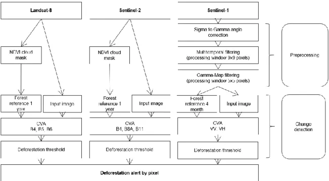
The methodological approach we used can be summarised as follows: (1) image pre-processing, (2) establishment of the forest reference, (3) Change Vector Analysis (CVA) application to all new images, and (4) application of appropriate thresholds to detect deforestation events (Figure 3).
Figure 3. Analysis method flowchart. The method performs the simultaneous analyses of three sensors to detect deforestation
1.4.3.1 Image preprocessing
1.4.3.1.1 Optical sensors
Sentinel-2 and Landsat-8 optical images were already converted to TOA reflectance by GEE. No atmospheric correction was applied to the images. According to Song et al. (2001 Song), training data from large areas and from different times of the year allow for avoiding atmospheric correction processes. Because the study area is located in a humid tropical forest, we observed that phenological events are much more subtle than the noticeable seasonal changes in forest cover that regularly take place in a drought-deciduous tropical forest or in a temperate deciduous forest. Therefore, no seasonal filters were employed in the current study.
1.4.3.1.2 Radar sensor
For Sentinel-1 images, images should be filtered to decrease speckle noise (Lê 2015), especially because CVA is a pixel-based comparison. Filters should conserve temporal and geometric information of deforestations. We decided to use a double filter approach as suggested by Quegan et al. (2000). With times series, a multi-temporal filter gives the advantage of preserving edges. The one-stage multi-temporal filter did not provide enough classification performance accuracy compared to that of two-stage multi-temporal and spatial filters (Quegan et al. 2000, Maghsoudi et al. 2012). Three steps were required for this pre-processing: (1) Gamma transformation; (2) Multi-temporal despeckle filter; and (3) and Gamma-map filter. (1) The gamma transformation that is
expressed by the following formula is a process that considers the angle of incidence that varies from one side of an image to the other:
𝛾0=cos 𝜃𝜎0 (1)
where gamma (γ) is the transformed pixel value in dB, sigma (σ0) is the initial pixel value in dB, and theta (θ) is the incidence angle, in radians.
(2) The multi-temporal despeckle filter (Quegan et al. 2000), acts over a spatial and temporal domain. This filter reduces speckle by relying upon information that is common to different dates, and while preserving the temporal information contained in each image. The multi-temporal filter code has been implemented with the help of the GEE help forum community. (3) The Gamma-map filter (Lopes et al. 1990), is an adaptive spatial filter, which smooths the homogeneous zones while preserving edges.
1.4.3.2 The forest references
References represent the time average signals of non-affected forest pixels, which are compared with each new image in order to determine whether a change has occurred or not. To create forest references, we filtered out clouds from the Sentinel-2 and Landsat-8 images. We found that cloud masks that were available in GEE missed several clouds and shadows; therefore, we designed a simple mask from conventional normalised vegetation index (NDVI; Rouse 1974). NDVI values below 0.6 were found to mostly refer to clouds and shadows, but they also included bare soil, urban areas, and water; vegetation pixels were mostly excluded. To obtain complete cover for the forest reference throughout the study area, we averaged all images for the previous year (2016). In contrast, Sentinel-1 images are not affected by cloud cover, therefore, we averaged only 4 months of pre-processed images to obtain the reference.
1.4.3.3 Change vector analysis
Our research applied Change Vector Analysis over the three sensors to detect the deforestation. CVA is a change detection per pixel method that is commonly used with optical images (Phua et al. 2008, Fernandes et al. 2014), but it is an innovative approach in the use of radar. Indeed, speckle noise of the radar sensor makes it difficult to implement the change detection process per pixel (Qi et al. 2015). To overcome the issue, the
For each pixel, we calculated the magnitude and the direction of change between the forest reference image and a new image (Malila 1980, Thonfeld et al. 2016). The magnitude is the Euclidean distance between the spectral values of 2 images that are positioned in 3-band spectral space. This length indicates the presence of change between the initial image and the new image. The direction is the angle projected in all the axes (Figure 4). The direction of change provided the change type, i.e. whether it is a cloud, a shadow or a deforestation event. To allow visual interpretation, we separated each pair of bands for the angle calculation. Formulae that were used for these calculations are:
𝜇 = √(Δ𝑅
Y) ² + (Δ𝑅
X)
2+ (𝛥𝑅
Z)
2(2)
𝛼 = arctg (
∆𝑅
Y∆𝑅
X) and arctg (
∆𝑅
Z∆𝑅
X) and arctg (
∆𝑅
Z∆𝑅
𝑌) (3)
where (2) μ is the magnitude of change, and (3) α is the direction of change. Δ𝑅Y is the difference between the spectral value of 2 images for band Y, Δ𝑅X is the difference between the spectral value of 2 images for band X.
If a third band is used, 𝛥𝑅Z is the difference between the spectral value of 2 images for band Z. Radiometric
bands or polarization bands X, Y and Z were defined, depending upon the sensor.
Figure 4. (a) Representation of change vector in two-band radiometric change space (for Sentinel-1), (b) Representation of change vector in three-band radiometric change space (for Sentinel-2 and Landsat-8).
A great advantage of using CVA is that clouds and shadows are detected as a specific change; consequently, we did not have to process cloud masks for each new input image.
To facilitate visualisation and interpretation, we used three bands to process the vector analyses for the optical images. Change information could also be located in other bands, but after analysed correlation between the bands, we found that three bands were sufficient. The red, near-infrared (NIR) and Shortwave Infrared (SWIR) bands were chosen for deforestation detection because of their ability to strongly segregate forests or clouds from bare soil. We used similar bands between Landsat-8 and Sentinel-2. For NIR, B8A from Sentinel-2 was used, because it is closest to band 5 of Landsat-8 (Mandanici and Bitelli 2016). Red was defined by band 4 for the two sensors, while SWIR was defined by band 6 in Landsat-8 and by band 11 for Sentinel-2, respectively. To find the threshold on magnitude and angles for the optical sensor, we created seven classes of change: no change (forest stayed forest), deforestation (forest became bare soil), various covered forest, various fog-covered bare soil, regrowth (new vegetation in bare soil), various clouds, and various shadows. For the Sentinel-1 radar sensor, we focused on 2 classes of change; no change (forest stays forest) and deforestation (forest became bare soil), determined from the image date against the date of deforestation.
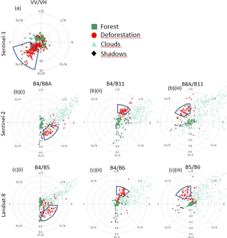
The length and three angles between the forest reference and deforestation were calculated and displayed in a polar coordinate plot as a function of change class to determine the best alert threshold for each angle combination (Figure 5). For the Sentinel-1 radar sensor, we used polarization bands available, VV and VH, to find the length and angle of the vector.
Figure 5. Figure (a) illustrates the VV (vertical/vertical) and VH (vertical/horizontal) bands for Sentinel-1. Figure (b) corresponds to Sentinel-2 sensors, with (b)(i) angle Band 4/Band 8A, (b)(ii) angle Band 4/Band 11 and (b)(iii) angle Band 8A/Band 11. Figure (c) corresponds to Landsat-8 sensors, with (c)(i) angle Band 4/Band 5, (c)(ii) angle Band 4/Band 6 and (c)(iii) angle Band 5/Band 6. Polar coordinate plots that were obtained by applying CVA, against 15 reference forest polygon averages. Green represents no change, red represent deforestation events, and blue are samples covered by cloud. The blue polygon indicates the deforestation threshold. Black dash polygons represent other examples of thresholds.
1.4.3.4 Threshold to detect deforestation
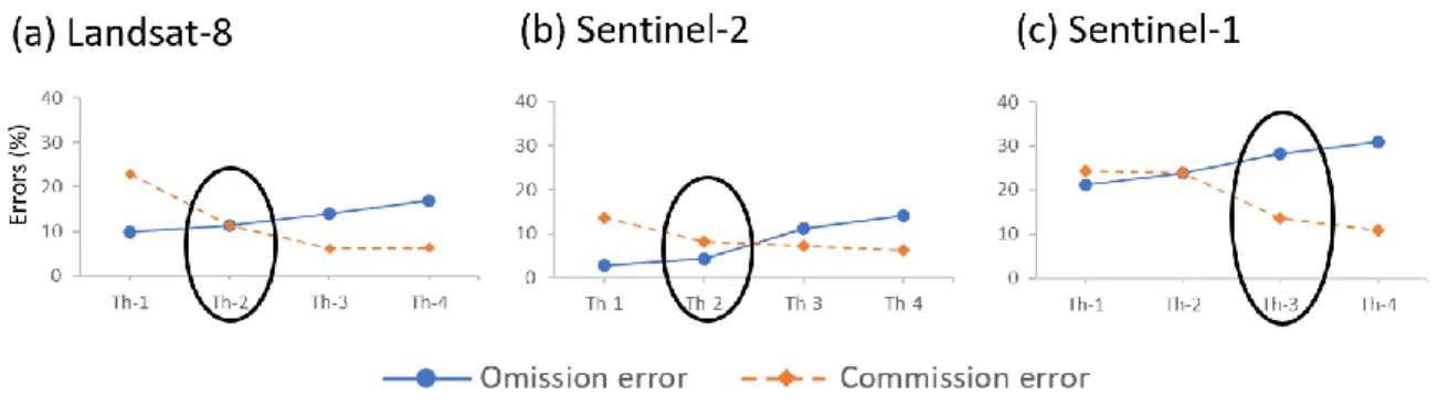
To identify the optimal detection rate, we used a trial-and-error approach. We selected a threshold which allowed most of the polygons to be detected but corresponded to a low false detection rate (Figure 6), which is essential for real-time alert purposes (Reiche and all. 2018). Bands used for Sentinel-2 were the same as for Landsat 8 (Mandanici and Bitelli 2016), but we found different thresholds for the two sensors.
Figure 6. Spatial accuracy (omission and commission errors) of the deforestation class as a function of four examples of threshold values, separately for (a) Landsat-8, (b) Sentinel-2 and (c) Sentinel-1. Thresholds annotations correspond to the parameters shown in Figure 5. Surrounding thresholds were used in our study.
Once the decision tree triggered the alert, the individual results are merged together to obtain a single image with all pixels detected as deforestation during the study period. This combination is performed for each sensor and at each multi-sensor level.
The change detection algorithm was coded in Google Earth Engine and applied throughout the Sabah state between 1 January 2017 and 31 May 2018 (Figure 7).
Figure 7. (a) Deforestation events detected at the multi-sensor level during the 17 months monitoring period in Sabah. (b) Deforestation events detected at the multi-sensor level during the 5 months monitoring period in Sumatra study area.
Two approaches are used to evaluate results: (1) A polygon level approach is analysed by deforestation events. When at least one pixel is found inside the validation polygon we considered the deforestation event to be
a false detection, and (2) A pixel-based approach to measure the capacity of detecting at small scale deforestation. The pixel accuracy is adjusted according to the proportion of each class in Sabah (Olofsson et al. 2014).
Only the pixel-based approach method was applied over the Sumatra area of interest between 1 January 2018 and 31 May 2018 (Figure 7).
1.5 Results and discussions
1.5.1 Change detection accuracy
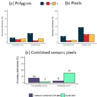
With regards to the polygons level approach, the three sensors had a high consensus of accuracy (Figure 8). Sentinel-1 radar showed the highest degree of omission error (20 polygons undetected) compared to optical sensors, which detected more deforestation events. Sentinel-2 and Landsat-8 showed best results with commission errors of 4% and 11%, respectively. In the pixel focus, all sensors had a higher omission error, which showed that only a relatively small number of pixels had been detected for each deforestation event. However, after combining the 3 sensors, the omission error decreased to 6%.
Figure 8. Comparative analysis of deforestation omission, and commission error for the three sensors corresponding to the best thresholds. (a) Corresponds to the polygons level approach, and (b) to the pixel-based adjusted area. (c) Represent the multi-sensor analysis in pixel-based adjusted area and its comparison with GLAD alert detection (Hansen et al. 2016). Numerical values on the histogram bars represent exact percentage values.
Sentinel-1 radar had greater commission error than the optical sensors. Sentinel-2 and Landsat-8 performed better in relation to the commission error in the pixel approach compared to the polygons focus, which showed that only a few pixels were falsely detected.
A final result combining all the sensors from the 17 months study period was compared with the GLAD (Global Land Analysis & Discovery) alert system during that same time frame (Hansen et al. 2016) (Figure 8). With 6% of omission error, our method provided a better detection of the deforestation pixel than GLAD (37% of omission error). On the other hand, the GLAD alert generated fewer false detections (3% of commission error).
False detections that occurred in the intact forest were mainly due to artefactual pixels located at the border of the tiles for Sentinel-1 or Sentinel-2. Further, half of the forest polygons corresponding to mangrove (10% of our plots) were detected as false detections. Excluding mangrove from the study area would have likely improved the commission error.
Of the 71 deforestation validation polygons, only 3 were omitted by Sentinel-2 optical. Landsat-8 missed 8 polygons during the analysis period. Only two deforestations event were not detected by any sensor. The spectral response of those events could be different, due to soil type or the progress of field preparation. Sentinel-1 radar yielded the poorest statistical results, likely a consequence of its geometric distortion and speckle noise not completely corrected by preprocessing filters. In addition, moisture and roughness variation of the bare soil during the plantation process can create difficulties to detect deforestation events. Comparatively to optical sensors, radar was not as valuable for detection deforestation.
1.5.2. Detection responsiveness as a function of cloud cover
Sabah is characterised by a high cloud-cover season between December and March, which affects optical images (Figure 1). We compared the reaction time for detecting deforestation as a function of the density of cloud cover (Figure 9). Based upon known deforestation dates, 9 polygons were deforested during the high cloud-cover season, while 54 were deforested during low cloud-cover season. Results show that Sentinel-1 radar detection delay was of a similar order of magnitude throughout the year. Optical sensors more than doubled the time period for the first detection during the peak cloudy season. During the low cloud-cover season, Landsat-8 attained the first detection at around 11.5 days. The median of the first detection was 8 ± 4.6 days when we combined all sensors throughout the study period.
Figure 9. Days of the first detection after deforestation events (estimates) across sensors, for (a) high cloud-cover season and (b) low cloud-cover season. The thick horizontal line within the box-plots represents the median (50th percentile) of each sensor. The box-plots themselves delimit the first and third quartiles (25th and 75th percentiles) and the whiskers (vertical dashed lines) indicate the 10th and 90th percentiles. Open circles represent outliers (i.e. values that are beyond 1.5 times the interquartile range.
These results support the relevance of including Sentinel-1 radar in near real-time detection of deforestation events throughout the year in areas subject to high cloud cover.
1.5.3. Temporal evolution of detection
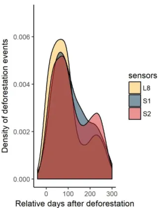
Most deforestation events were detected between 0 and 100 days after the disturbance (Figure 10). After 100 days (over 3 months), the number of detections decreased until 300 days (10 months) had passed, after which polygon deforestation events were no longer detected. After about 200 days, the number of detections increased again, for a new hundred days.
Figure 10. Density of deforestation events that were detected as a function of time following deforestation (estimated). These results allowed us to visualise the distribution of detection responses before and after deforestation. Zero is the estimated first date of forest cover loss.
Dynamic cover crop species can completely cover soil 4–5 months after the plantation (Skerman 1982), and this dynamic growth rate is consistent with the decrease of the detection of bare soil after 3 months. After that, young palm trees are planted, which may seem like a new deforestation.
1.5.4. Frequency of detection
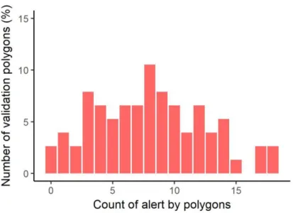
For an operational detection system, false detection must be avoided as much as possible. False detections were found to be mostly due to artefact in the imagery and occurred a maximum of 3 times per validation polygon in a period of 17 months. Hence, to confirm a deforestation event, pixels should be detected at least 3 times to eliminate the potential for random errors. We wondered if deforestation events were detected frequently enough to allow this confirmation. The number of validation polygons (as percentages) are presented in Figure 11 as a function of the number of times that they were detected over a period of 100 days following forest clearing. Two of the 71 polygons were never detected during the analysis interval, and three others were only detected once; 18% of the validation polygons were detected fewer than 4 times, while half of the polygons were detected less than 11 times each. This frequency was possible because detection results from all three sensors were used, thereby supporting the interest of combining radar and optical sensors in this context.
Figure 11. Number of validation polygons (as percentages) as a function of the number of times that they were detected over a period of 100 days following forest clearing.
The accumulation of 3 detections to reduce commission error increases the omission error rate to 24% and decreases the commission rate to 1% (instead of 6% of omission error and 18% of commission error).
1.5.5. Validation in Sumatra
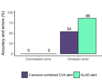
We implemented our detection method in the Sumatra area between 1 January and 31 May 2018 (Figure 12). We estimated that this period should correspond to the deforestation events of areas captured by drone imagery in early May. Results from the confusion matrix (Figure 13) yielded a high number of omission errors (53%) in deforestation detection. None of the 29 forest points were false detections (commission error of 0%). The low number of results could be attributed to a delay between deforestation events and alert detection being too short if the deforestations occurred in early May, or by the state of the forest before the disturbance. Indeed, about 10 points had not been detected by our method but appeared to be bare soil in the imagery. However, these areas have been previously disturbed and did not represent undisturbed forest canopy. This result shows that our methodology is well oriented to only detect disturbance of intact forests.
Figure 12. (a, b, c) Examples of drone photographs that were taken 9 May 2018. (d) Illustration of deforestation detection: In red, pixels detected as deforested by our method, between 1 January and 31 May 2018, over a Planet image of 18 February 2018. Points are the position of the drone pictures, green points are forest (a), and pink points are bare soil (b and c).
Figure 13. Comparative analysis of deforestation omission and commission errors and overall accuracy of the method presented in this paper versus that provided by GLAD forest alert detection (Hansen et al. 2016). Numerical values on the histogram bars represent exact percentage values.
We compared our results against the GLAD alert system (Hansen et al. 2016). We applied the confusion matrix to our field plots versus possible GLAD alert pixels. Most points were not detected by the GLAD system (omission error of 86%) compared to our method. Both methods demonstrated no commission error.
When we confined the use of our method to Landsat-8 only, we obtained results that were similar to the GLAD alerts (omission error of 81%). This comparison suggests there is high relevance in using the three sensors for improving the change detection process in these forested areas.
1.6 Conclusion
The objective of this research was to assess to what extent could we improve near real-time deforestation observations by combining Landsat-8 and Sentinel-2 optical sensors, and the Sentinel-1 radar sensor over Southeast Asia. By using Change Vector Analysis method over Sabah, Malaysia, all sensors separately yielded reasonable statistical results. With 14% of commission error and 28% of omission error, we consider the Change Vector Analysis method in detecting deforestation effective with Sentinel-1, despite speckle noise. A comparison between our method (yielding 54% omission error) and the GLAD alert system (86% omission error) (Hansen et al. 2016) in a smaller area in Sumatra, confirms the utility of combining the three sensors for improved detection. Sensors have different characteristics, which can provide a high-performance operational system when used together. By comparing pixel and polygon metrics errors, we observed that only a small part of the deforestation was detected by each sensor, and the combination allowed for better detection (6% of omission error). Sentinel-2 and Landsat-8 optical data are more accurate in the detection of deforestation events. During the high cloud-cover season, while optical sensors took about twice the time to detect deforestation, the reaction time of Sentinel-1 remained about 20 days. Using the three sensors provided informative detection results during the first 100 days after the deforestation event, before bare soils were covered by legume crop. Almost every deforestation event was detected by our method (97%), but results were affected by several false detections (25%) mostly generated by imagery artefacts. Those false detections could be avoided by adding a system of confirmation using multiple detections per pixel.
1.7 References
Asner, G. P., P. G. Brodrick, N. R. Christopher Philipson, R. E. Vaughn, D. E. Martin, and J. H. Knapp. 2018. “Mapped Aboveground Carbon Stocks to Advance Forest Conservation and Recovery in Malaysian Borneo.”
Austin, K. G., A. Mosnier, J. Pirker, I. McCallum, S. Fritz, and P. S. Kasibhatla. 2017. “Shifting Patterns of Oil Palm Driven Deforestation in Indonesia and Implications for Zero-Deforestation Commitments.” Land Use Policy 69 (December): 41–48. doi:10.1016/j.landusepol.2017.08.036.
Awalludin, M. F., O. Sulaiman, R. Hashim, W. N. Aidawati, and W. Nadhari. 2015. “An Overview of the Oil Palm Industry in Malaysia and Its Waste Utilization through Thermochemical Conversion, Specifically via Liquefaction.” Renewable and Sustainable Energy Reviews 50 (October): 1469–1484. doi:10.1016/j.rser.2015.05.085.
Berry N. J., Phillips O. L., Lewis S. L., Hill J. K., Edwards D. P., Norhayati A., David M., et al. 2010. “The High Value of Logged Tropical Forests: Lessons from Northern Borneo”. Biodiversity Conservation 19: 985–997. doi:10.1007/s10531-010-9779-z.
Bryan, J. E., Shearman, P. L., Asner, G. P., Knapp, D.E., Aoro, G., and Lokes B. 2013. “Extreme Differences in Forest Degradation in Borneo: Comparing Practices in Sarawak, Sabah, and Brunei.” PloS one 8 (7): e69679. doi:10.1371/journal.pone.0069679.
Evans, L. J., G. P. Asner, and B. Goossens. 2018. “Protected Area Management Priorities Crucial for the Future of Bornean Elephants.” Biological Conservation 221 (May): 365–373. doi:10.1016/j.biocon.2018.03.015. Fernandes, P. J. F., L. F. de Almeida Furtado, and R. E. S. Girão. 2014. “Change Vector Analysis to Detect Deforestation and Land Use/Land Cover Change in Brazilian Amazon.” Brazilian Geographical Journal:
Geosciences and Humanities Research Medium 5 (2): 371–387.
https://dialnet.unirioja.es/servlet/articulo?codigo=4995484
Gaveau, D. L. A., D. Sheil, M. A. Husnayaen, S. A. Salim, M. Ancrenaz, P. Pacheco, and E. Meijaard. 2016. “Rapid Conversions and Avoided Deforestation: Examining Four Decades of Industrial Plantation Expansion in Borneo.” Scientific Reports 6 (September): 32017. doi:10.1038/srep32017.
Gorelick, N., M. Hancher, M. Dixon, S. Ilyushchenko, D. Thau, and R. Moore. 2017. “Google Earth Engine: Planetary-Scale Geospatial Analysis for Everyone.” Remote Sensing of Environment, Big Remotely Sensed Data: Tools, Applications and Experiences 202 (December): 18–27. doi:10.1016/j.rse.2017.06.031.
Hammer, D., R. Kraft, and D. Wheeler. 2014. “Alerts of Forest Disturbance from MODIS Imagery.” International
Hansen, M. C., A. Krylov, P. V. Alexandra Tyukavina, S. T. Potapov, B. Zutta, S. Ifo, B. Margono, F. Stolle, and R. Moore. 2016. “Humid Tropical Forest Disturbance Alerts Using Landsat Data.” Environmental Research
Letters 11 (3): 034008. doi:10.1088/1748-9326/11/3/034008.
Hansen, M. C., S. V. Stehman, P. V. Potapov, T. R. Loveland, J. R. G. Townshend, R. S. DeFries, K. W. Pittman, et al. 2008. “Humid Tropical Forest Clearing from 2000 to 2005 Quantified by Using Multitemporal and Multiresolution Remotely Sensed Data.” Proceedings of the National Academy of Sciences 105 (27): 9439– 9444. doi:10.1073/pnas.0804042105.
Hansen, M. C., and T. R. Loveland. 2012. “A Review of Large Area Monitoring of Land Cover Change Using Landsat Data.” Remote Sensing of Environment, Landsat Legacy Special Issue 122 (July): 66–74. doi:10.1016/j.rse.2011.08.024.
Houborg, R., and M. F. McCabe. 2018. “A Cubesat Enabled Spatio-Temporal Enhancement Method (CESTEM) Utilizing Planet, Landsat and MODIS Data.” Remote Sensing of Environment 209 (May): 211–226. doi:10.1016/j.rse.2018.02.067.
Houghton, R. A., B. Byers, and A. A. Nassikas. 2015. “A Role for Tropical Forests in Stabilizing Atmospheric CO2.” Nature Climate Change 5 (12): 1022–1023. doi:10.1038/nclimate2869.
Jacquemard, J. C. 2013. Le palmier à huile en plantation villageoise. Versailles: Quae.
Joshi, N., M. Baumann, A. Ehammer, R. Fensholt, K. Grogan, P. Hostert, M. R. Jepsen, et al. 2016. “A Review of the Application of Optical and Radar Remote Sensing Data Fusion to Land Use Mapping and Monitoring.”
Remote Sensing 8 (1): 70. doi:10.3390/rs8010070.
Khun, V., and N. Sasaki. 2014. “Re-Assessment of Forest Carbon Balance in Southeast Asia: Policy Implications for REDD+.” Low Carbon Economy 05 (04): 153. doi:10.4236/lce.2014.54016.
Koh, L. P., J. Miettinen, S. C. Liew, and J. Ghazoul. 2011. “Remotely Sensed Evidence of Tropical Peatland Conversion to Oil Palm.” Proceedings of the National Academy of Sciences 108 (12): 5127–5132. doi:10.1073/pnas.1018776108.
Lê, T. T. 2015. “Extraction d’Informations de changement à partir des Séries Temporelles d’Images Radar à Synthèse d’Ouverture.” PhD diss., Université de Grenoble Alpes, STIC Traitement de l’Information, 174. Lehmann, E. A., P. Caccetta, K. Lowell, A. Mitchell, Z.-S. Zhou, A. Held, T. Milne, and I. Tapley. 2015. “SAR and Optical Remote Sensing: Assessment of Complementarity and Interoperability in the Context of a Large-Scale
Operational Forest Monitoring System.” Remote Sensing of Environment 156 (January): 335–348. doi:10.1016/j.rse.2014.09.034.
Lopes, A., E. Nezry, R. Touzi, and H. Laur. 1990. “Maximum a Posteriori Speckle Filtering and First Order Texture Models in SAR Images.” Paper presented at Geoscience and Remote Sensing Symposium, 1990. IGARSS ‘90. ‘Remote Sensing Science for the Nineties’., 10th Annual International 2409-2412 doi:10.1109/IGARSS.1990.689026.
Maghsoudi, Y., M. J. Collins, and D. Leckie. 2012. “Speckle Reduction for the Forest Mapping Analysis of Multi-Temporal Radarsat-1 Images.” International Journal of Remote Sensing 33 (5): 1349–1359. doi:10.1080/01431161.2011.568530.
Malaysian Palm Oil Board. 2017. “Economics and Industry Development Division.” Accessed June 2018. http://bepi.mpob.gov.my/index.php/en/statistics/area.html
Malila, W. 1980. “Change Vector Analysis: An Approach for Detecting Forest Changes with Landsat.” LARS Symposia, January. https://docs.lib.purdue.edu/lars_symp/385
Mandanici, E., and G. Bitelli. 2016. “Preliminary Comparison of Sentinel-2 and Landsat 8 Imagery for a Combined Use.” Remote Sensing 8 (12): 1014. doi:10.3390/rs8121014.
May-Tobin, C., D. Boucher, E. Decker, G. Hurowitz, J. Martin, K. Mulik, S. Roquemore, and A. Stark. 2012.
Recipes for Sucess. Solutions for Deforestation-Free Vegetable Oils. MA, USA: Union of Concerned Scientists
(UCS). https://www.ucsusa.org/sites/default/files/legacy/assets/documents/global_warming/Recipes-for-Success.pdf
Miettinen, J., C. Shi, and S. C. Liew. 2016. “Land Cover Distribution in the Peatlands of Peninsular Malaysia, Sumatra and Borneo in 2015 with Changes since 1990.” Global Ecology and Conservation 6 (April): 67–78. doi:10.1016/j.gecco.2016.02.004.
“MODIS Collection 6 NRT Hotspot/Active Fire Detections MCD14DL.” https://earthdata.nasa.gov/firms Olofsson, Pontus, G. M. Foody, M. Herold, S. V. Stehman, C. E. Woodcock, and M. A. Wulder. 2014. “Good Practices for Estimating Area and Assessing Accuracy of Land Change.” Remote Sensing of Environment 148 (May): 42–57. doi:10.1016/j.rse.2014.02.015.