Etudes expérimentales et modélisation du comportement de phase et des propriétés de transport des mélanges liés à la capture et au stockage du carbone

(1)

HAL Id: tel-01668568

https://pastel.archives-ouvertes.fr/tel-01668568

Submitted on 20 Dec 2017

HAL is a multi-disciplinary open access

archive for the deposit and dissemination of sci-entific research documents, whether they are pub-lished or not. The documents may come from teaching and research institutions in France or abroad, or from public or private research centers.

L’archive ouverte pluridisciplinaire HAL, est destinée au dépôt et à la diffusion de documents scientifiques de niveau recherche, publiés ou non, émanant des établissements d’enseignement et de recherche français ou étrangers, des laboratoires publics ou privés.

comportement de phase et des propriétés de transport

des mélanges liés à la capture et au stockage du carbone

Alfonso Gonzalez Perez

To cite this version:

Alfonso Gonzalez Perez. Etudes expérimentales et modélisation du comportement de phase et des propriétés de transport des mélanges liés à la capture et au stockage du carbone. Milieux fluides et réactifs. Université Paris sciences et lettres; Heriot-Watt university (Edimbourg, GB), 2016. Français. �NNT : 2016PSLEM059�. �tel-01668568�

(2)

THÈSE DE DOCTORAT

de l’Université de recherche Paris Sciences et Lettres

PSL Research University

Préparée à MINES ParisTech

Etudes expérimentales et modélisation du comportement de phase et

des propriétés de transport des mélanges lies à la capture et au

stockage du carbone

COMPOSITION DU JURY :

M. Jean Philippe PASSARELLO Université Paris 13 Nord, Président M. Jean Luc DARIDON 

Université de Pau, Rapporteur M. Richard GRAHAM

University of Nottingham, Rapporteur M. Manuel MARTÍNEZ PIÑEIRO Universidade de Vigo, Examinateur M. Francois MONTEL TOTAL,  Examinateur M. Patrice PARICAUD Ensta-ParisTech, Examinateur M. Antonin CHAPOY

Heriot-Watt University, Examinateur M. Christophe COQUELET

Mines-ParisTech, Examinateur

Soutenue par

Alfonso

GONZALEZ PEREZ

le 30 Novembre 2016

h

Ecole doctorale

n°

432

SCIENCES DES MÉTIERS DE L'INGÉNIEUR

Spécialité

ENERGÉTIQUE ET PROCÈDES

Dirigée par Christophe COQUELET

et Antonin CHAPOY

(3)

The work presented in this manuscript has been developed as part of my PhD studies at PSL-Mines ParisTech and Heriot-Watt University under the supervision of Prof. Christophe Coquelet, Dr. Patrice Paricaud and Dr. Antonin Chapoy, between October 2013 and October 2016. Phase behaviour models implemented in the in-house PVT software of the research group were used throughout this work. Part of the material in this manuscript has been presented or published elsewhere before; the list of publications concerning the studies described in this manuscript is given in LIST OF PUBLICATIONS BY THE CANDIDATE.

Alfonso González Pérez October 2016

(4)

(5)

It is now widely accepted that anthropogenic CO2 emissions produced from the burning

of fossil fuels are responsible for the apparent rapid rise in global temperatures recorded over the past century. Worldwide concerns over the threat of global warming have motivated the majority of industrialised countries into working to reduce carbon emissions. CO2 storage in depleted reservoirs and its application in Enhanced Oil/Gas

Recovery (EOR) are among techniques being suggested for reducing the emission of this greenhouse gas. The main aim of this research is to develop a thermodynamic model from an accurate equation of state (EoS) for typical components of reservoir fluids and flue gases. The SAFT-VR Mie EoS was selected to study the phase behaviour and transport properties of mixtures related to carbon capture and storage (CCS). Four EoSs have been compared (PR, SRK, PC-SAFT and SAFT-VR Mie) by modelling density and vapour-liquid equilibria (VLE) data from the literature of 22 pure components and 108 binary systems of gases (CO2, H2S, N2, O2, Ar, CO and SO2),

n-alkanes and aromatics.

Isothermal vapour-liquid equilibrium of H2S - Ar binary system was determined

experi-mentally at three temperatures from 273 to 323 K. Densities of five H2S binary systems

(three CH4-H2S systems with 13, 18 and 28 % of acid gas, C2H6 - 34% H2S and C3H8 -

13% H2S) were measured continuously at 3 temperatures (253, 273 and 293 K) and at

pressures up to 30MPa, using a vibrating tube densitometer, Anton Paar DMA 512. Following the same technique, the density of the ternary system 42% CO2, 40% CH4

and 18% H2S was measured at pressures ranging from 0.2 to 31.5 MPa and at 6

temperatures between 253 and 353 K.

Three transport properties were modelled with SAFT-VR Mie and two models based on density predictions from the EoS. Density, viscosity and interfacial tension (IFT) of CO2-rich systems were calculated by the SAFT-EoS (density), TRAPP model

(viscosity) and DGT (IFT), for system of interest to CCS. Densities and viscosities of a multicomponent mixture of 50% CO2, 40% CH4 and 10% of other impurities were

measured at 5 temperatures between 283 and 423 K and at 2.5-150 MPa pressure range, using an Anton Paar densitometer and the capillary tube technique for viscosity measurements. These experimental data continued studying the impact of impurities on the viscosity and density of CO2-rich systems.

(6)

(7)

LIST OF PUBLICATIONS BY THE CANDIDATE ... v

LISTS OF TABLES ... vii

LISTS OF FIGURES ... xiii

NOMENCLATURE ... xxi

CHAPTER 1 : INTRODUCTION ... 1

1.1 Scope ... 1

1.2 Carbon Capture and storage ... 2

1.2.1 Carbon Capture ... 3

1.2.2 Transport of CO2 ... 4

1.2.3 Storage... 6

1.3 Goals ... 8

1.4 Thesis overview ... 9

CHAPTER 2 : EXPERIMENTAL STUDY ... 11

2.1 Introduction ... 11

2.2 Vapour-liquid equilibria of H2S - Ar ... 13

2.2.1 Materials ... 13

2.2.2 Equipment description ... 13

2.2.3 Calibration procedure and uncertainty ... 15

2.2.4 Experimental procedure ... 15

2.2.5 Results ... 16

2.3 Density measurements of C1-C3 and H2S binary systems ... 17

2.3.1 Sample preparation... 18

(8)

2.4 Density measurements of the CO2–CH4–H2S ternary system... 23

2.4.1 Sample preparation... 24

2.4.2 Calibration procedure ... 24

2.4.3 Results ... 25

2.5 Density and viscosity measurements of a multicomponent CO2–rich mixture ... 26

2.5.1 Materials ... 26

2.5.4 Experimental procedure ... 29

2.5.5 Results ... 30

CHAPTER 3 : THERMODYNAMIC BACKGROUND ... 33

3.1 Intermolecular forces ... 33

3.2 Phase behaviour ... 37

3.3 Equations of state ... 39

3.3.1 Evolution of EoSs ... 39

3.3.2 SAFT Equations of State ... 42

CHAPTER 4 : MODELLING PHASE AND VOLUMETRIC BEHAVIOURS ... 53

4.1 SAFT-VR Mie ... 53

4.1.1 Modelling aspects and approaches ... 53

4.1.2 Description and formulation ... 56

4.1.3 Mie molecular parameters ... 63

4.2 Comparative study of EoSs ... 68

4.2.1 Cubic EoSs ... 68

4.2.2 SAFT-like EoSs ... 69

4.2.3 Results and discussion ... 71

4.2.4 Remarks and conclusions ... 94

4.3 SAFT-γ Mie ... 95

4.3.1 Modelling aspects and approach ... 96

4.3.2 SAFT-γ Mie modelling results ... 98

(9)

CHAPTER 5 : MODELLING TRANSPORT PROPERTIES WITH THE

SAFT-VR MIE EOS ... 105

5.1 Viscosity ... 105

5.1.1 TRAPP method ... 105

5.1.2 Results of viscosity modelling ... 110

5.2 Interfacial tension ... 114

5.2.1 Density Gradient Theory ... 114

5.2.2 Results of IFT modelling ... 118

5.3 Conclusions ... 125

CHAPTER 6 : MODELLING AND DISCUSSION OF EXPERIMENTAL MEASUREMENTS ... 127

6.1 Vapour-liquid equilibrium of H2S - Ar ... 127

6.1.1 Results ... 127

6.1.2 Conclusions ... 136

6.2 Density measurements of CH4 - H2S systems ... 137

6.2.1 Results ... 137

6.3 Density measurements of C2H6 + H2S and C3H8 + H2S ... 144

6.3.1 Results ... 144

6.4 Density measurements of CO2+CH4+H2S ternary system ... 148

6.4.1 Results ... 148

6.5 Density and viscosity measurements of a multicomponent CO2–rich mixture ... 152

6.5.1 Results ... 152

CHAPTER 7 : CONCLUSIONS AND FUTURE WORK ... 157

7.1 Modelling investigation ... 157

7.2 Experimental investigation... 159

(10)

A.1 Density and compressibility factor uncertainty ... 164

A.2 VLE data uncertainty ... 166

A.3 Viscosity uncertainty ... 167

APPENDIX B : EXPERIMENTAL DENSITY DATA ... 169

APPENDIX C : CUBIC EQUATIONS OF STATE ... 191

C.1 SRK EoS ... 191

C.2 PR EoS ... 191

APPENDIX D : PC-SAFT EQUATION OF STATE ... 193

APPENDIX E : mBWR EQUATION OF STATE ... 197

APPENDIX F : EXECUTIVE SUMMARY ... 199

APPENDIX G : PPEPPD Conference Poster ... 209

(11)

LIST OF PUBLICATIONS BY THE CANDIDATE

A. Gonzalez, A. Valtz, P. Paricaud, C. Coquelet, A. Chapoy, Experimental and modelling study of the densities of the hydrogen sulphide + methane mixtures at 253, 273 and 293

K and pressures up to 30 MPa, Fluid Phase Equilib. 427, 371–383 (2016).

A. Gonzalez, P. Paricaud, C. Coquelet, A. Chapoy, Comparative study of vapour-liquid equilibrium and density modelling of mixtures related to carbon capture and storage with the SRK, PR, PC-SAFT and SAFT-VR Mie equations of state for industrial uses, (in preparation).

A. Gonzalez, A. Valtz, P. Paricaud, C. Coquelet, A. Chapoy, Vapour–liquid equilibrium data for the argon (Ar) + hydrogen sulphide (H2S) system at 273, 298 to 323 K, (in

preparation).

A. Gonzalez, A. Valtz, P. Paricaud, A. Chapoy, C. Coquelet, Experimental and modelling study of the density of one mixture of ethane + hydrogen sulphide and one mixture of propane + hydrogen sulphide at 253, 273 and 293 K and pressures up to 30 MPa.

A. Gonzalez Perez, L. Pereira, P. Paricaud, C. Coquelet, A. Chapoy, Modeling of transport properties using the SAFT-VR Mie equation of state, published and presented (oral) in SPE Annual Technical Conference and Exhibition (Paper # SPE-175051-MS), Houston, Texas, USA (2015).

A. Gonzalez Perez, P. Paricaud, C. Coquelet, A. Chapoy, Vapour-liquid equilibria and density modelling of CO2-rich systems with PC-SAFT and SAFT-VR Mie, presented (poster)

in 13th International Conference on Properties and Phase Equilibria for Products and Process Design (PPEPPD), Porto, Portugal (2016).

C. Coquelet, P. Stringari, M. Hajiw, A. Gonzalez Perez, L. Pereira, M. Nazeri, R. Burgass, A. Chapoy, Transport of CO2: Presentation of New Thermophysical Property

Measurements and Phase Diagrams, presented (poster) in 13th International Conference on Greenhouse Gas Control Technologies (GHGT), Lausanne, Switzerland (2016).

(12)

(13)

LISTS OF TABLES

Table 1.1. Example of composition specifications [11]. ... 5

Table 2.1. Vapour-liquid equilibrium (■) and density (□) data available in the literature for the binary systems studied in this work (NIST Databases [42,171]). ... 12

Table 2.2. Vapour–liquid equilibrium pressures, phase compositions for Ar (1) - H2S (2) mixtures and uncertainties of measurements (N: number of samples; and σ: Standard deviation). Uncertainty on temperature u(T) = 0.02 K and uncertainty on pressure u(P)= 0.002 MPa. ... 16

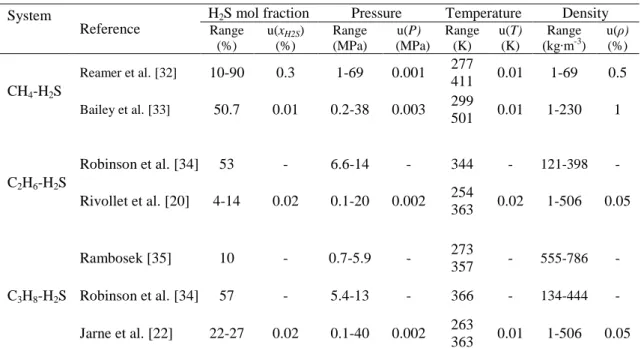
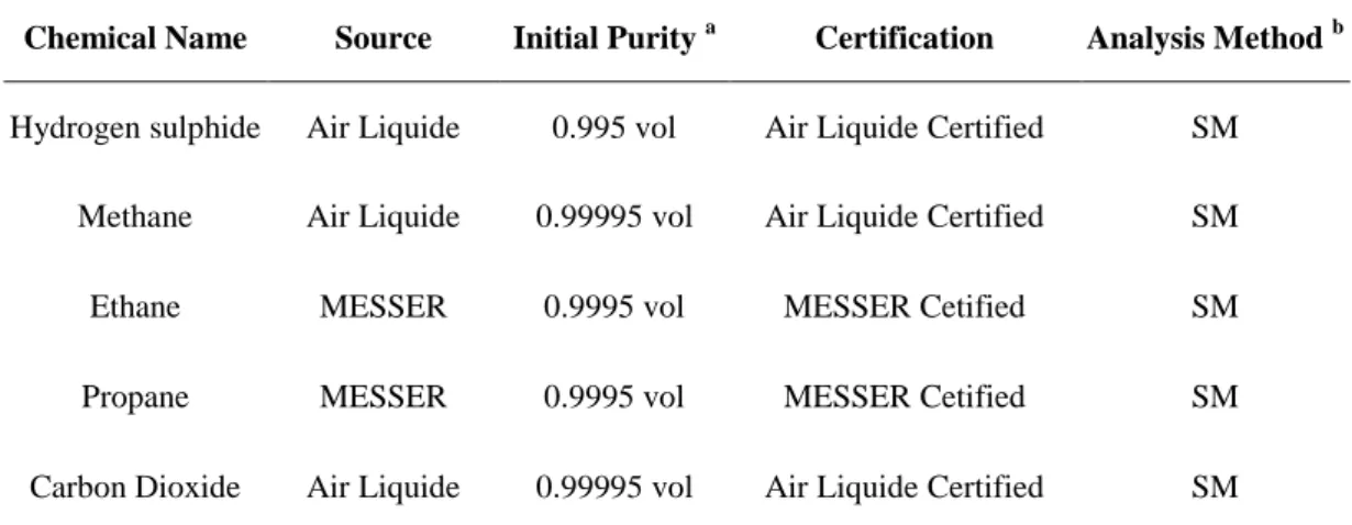
Table 2.3. Available experimental PTρx data in the literature with their uncertainties for the C1-C3 and hydrogen sulphide binary systems. ... 17 Table 2.4. Details of the chemicals, suppliers and purities of the components used in this study. ... 18

Table 2.5. Resulting compositions of the studied mixture of methane, ethane and propane with hydrogen sulphide. ... 19

Table 2.6. Composition of MIX4. ... 26

Table 2.7. Experimental results of the density and viscosity of MIX4. ... 31

Table 3.1. References of some of the most well-known SAFT versions (from Thermodynamic models for industrial applications) [119] ... 45

Table 3.2. Summary of the SAFT-VR versions ... 49

Table 3.3. Summary of published works of several SAFT + Group Contribution approach EoSs (from Thermodynamic models for industrial applications) [119] ... 52

Table 4.1. Reduced abscissas and weights of the ten-point Gauss-Legendre quadrature [161,162] ... 58

Table 4.2. Coefficients ϕi,n for Eq.4.38 and 4.49 ... 61 Table 4.3. SAFT-VR Mie pure-component parameters from the literature [72,90]. ... 64

Table 4.4. Mie molecular parameters for hydrogen sulphide, and average absolute deviation (%AAD) from experimental correlations [42] for the vapour pressure (Psat), the saturated-liquid density (ρsat) and the enthalpy of vaporization (ΔHv). ... 65

(14)

Table 4.5. Average absolute deviations (%AAD) in predictions (kij=0) and calculations (using regressed kij’s) of bubble pressures (ΔP

bubble

) and vapour phase compositions (Δy1) of CO2 + Comp2 binary systems with the SRK, PR, PC-SAFT and SAFT-VR Mie EoS. ... 75 Table 4.6. Average absolute deviations (%AAD) in predictions (kij=0) and calculations (using regressed kij’s) of bubble pressures (ΔP

bubble

) and vapour phase compositions (Δy1) of CH4 + Comp2 binary systems with the SRK, PR, PC-SAFT and SAFT-VR Mie EoS. ... 77 Table 4.7. Average absolute deviations (%AAD) in predictions (kij=0) and calculations (using regressed kij’s) of bubble pressures (ΔP

bubble

) and vapour phase compositions (Δy1) of C2H6 + Comp2 binary systems with the SRK, PR, PC-SAFT and SAFT-VR Mie EoS. ... 79 Table 4.8. Average absolute deviations (%AAD) in predictions (kij=0) and calculations (using regressed kij’s) of bubble pressures (ΔP

bubble

) and vapour phase compositions (Δy1) of N2 + Comp2 binary systems with the SRK, PR, PC-SAFT and SAFT-VR Mie EoS. ... 81 Table 4.9. Average absolute deviations (%AAD) in predictions (kij=0) and calculations (using regressed kij’s) of bubble pressures (ΔP

bubble

) and vapour phase compositions (Δy1) of H2S+ Comp2 binary systems with the SRK, PR, PC-SAFT and SAFT-VR Mie EoS. ... 82 Table 4.10. Summary of the average absolute deviations (%AAD) in bubble pressures (ΔPbubble) and vapour phase compositions (Δy1) predicted (kij=0) and calculated (kij≠0) by the SRK, PR, PC-SAFT and SAFT-VR Mie EoS. ... 84

Table 4.11. Average absolute binary interaction parameters and average sensitivities in the VLE calculations. ... 85

Table 4.12. Critical properties of CO2 predicted with PC-SAFT and SAFT-VR Mie and comparison with experimental data. ... 87

Table 4.13. Average (AAD%) and maximum (MAD%) absolute deviations in correlated single-phase fluid density by the SRK, SRK + Peneloux, PR, PR + Peneloux, PC-SAFT and SAFT-VR Mie models within 253-523 K and 0-150 MPa. ... 88

Table 4.14. Deviation in calculated density of CO2 + Comp2 systems by SRK, PR, PC-SAFT and PC-SAFT-VR Mie with and without volume correction. ... 89

Table 4.15. Deviation in calculated density of CH4 + Comp2 systems by SRK, PR, PC-SAFT and PC-SAFT-VR Mie with and without volume correction. ... 90

Table 4.16. Deviation in calculated density of C2H6 + Comp2 systems by SRK, PR, PC-SAFT and PC-SAFT-VR Mie with and without volume correction. ... 90

Table 4.17. Deviation in calculated density of N2 + Comp2 systems by SRK, PR, PC-SAFT and SAFT-VR Mie with and without volume correction. ... 91

(15)

Table 4.18. Deviation in calculated density of H2S + Comp2 systems by SRK, PR,

PC-SAFT and PC-SAFT-VR Mie with and without volume correction. ... 91

Table 4.19. Group parameters for the methyl and methylene functional groups [141]. ... 99

Table 4.20. Dispersion interaction εkl energies for the methyl and methylene functional groups [141]. ... 99

Table 4.21. Average absolute deviation of saturation pressures (PSAT) and saturated-liquid densities (ρSAT ) of alkanes series at reduced temperatures between 0.4 and 0.9 ... 100

Table 4.22. Deviation in calculated density of C2H6 + n-alkanes systems by SAFT-VR Mie and SAFT- γ Mie. ... 102

Table 4.23. Deviation in calculated density of n-decane + n-alkanes systems by SAFT-VR Mie and SAFT- γ Mie. ... 103

Table 5.1. Ei parameter SUPERTRAPP Model [50]. ... 106

Table 5.2. Coefficientes ai of the Ψη* for CO2. [195]. ... 109

Table 5.3. Coefficientes dij [195]. ... 110

Table 5.4. Literature experimental data for the viscosity of CO2-mixtures with N2, O2, and Ar. ... 110

Table 5.5. Average absolute deviation of the viscosity calculations. ... 111

Table 5.6. Average absolute deviation of the viscosity calculations. ... 114

Table 5.7. DGT influence parameters. ... 116

Table 5.8. Binary interaction parameters between CO2, n-butane and n-decane for the SAFT-VR Mie used in this work. ... 118

Table 5.9. Average absolute deviations (%AAD) between experimental and predicted IFT using the DGT+SAFT-VR Mie model (this work) and the results from Pereira et al. using the VT-PPR78 with the Parachor and DGT models [219]. ... 123

Table 6.1. Regressed BIPs for the Ar+H2S system using the PR and SAFT-VR Mie EoSs. ... 128

Table 6.2. Average absolute deviations (%AAD) of bubble pressures (ΔPbubble) and vapour phase compositions (Δy1) of Ar-H2S system with the PR and SAFT-VR Mie EoS. ... 129

Table 6.3. Values of the adjusted binary parameters (τij and kij) and deviation (%AAD) in bubble pressure and vapour composition at each studied temperature using the PR EoS with the W-S mixing rules. ... 133

(16)

Table 6.4. Average absolute deviations (%AAD) between the studied models and the densities measured in this work. ... 138

Table 6.5. Average absolute deviation (%AAD) between the available experimental data and the studied models. ... 139

Table 6.6. Regressed parameters for the calculation of the second virial coefficient B, condition ranges and AAD deviations between the correlation and experimental compressibility factors. ... 142

Table 6.7. Average absolute deviation (%AAD) between the available experimental data and the studied models. ... 145

Table 6.8. Binary interaction parameters between CH4, CO2 and H2S for the PR and SAFT-VR Mie EoSs. ... 148

Table 6.9. Average absolute deviations (%AAD) between the studied models and the densities measured in this work. ... 149

Table 6.10. Average absolute deviation (%AAD) between the measured density data and the studied models. ... 152

Table 6.11. Average absolute deviation in viscosities calculations with the SUPERTRAPP and CO2-SUPERTRAPP models using predicted and experimental densities. ... 153

Table B.1. Experimental results of the 0.8685 mol CH4 + 0.1315 mol H2S system at 253K, u(xH2S)=0.0006, u(T)= 0.03 K, u(P)= 0.003 MPa for pressures up to 5 MPa and u(P)= 0.005 MPa for pressures from 5 to 30 MPa. ... 169

Table B.2. Experimental results of the 0.8685 mol CH4 + 0.1315 mol H2S system at 273K, u(xH2S)=0.0006, u(T)= 0.03 K, u(P)= 0.003 MPa for pressures up to 5 MPa and u(P)=0.005 MPa for pressures from 5 to 30 MPa. ... 170

Table B.4. Experimental results of 0.8197 mol CH4 + 0.1803 mol H2S system at 253K, u(xH2S)=0.0008, u(T)= 0.03 K, u(P)= 0.003 MPa for pressures up to 5 MPa and u(P)= 0.005 MPa for pressures from 5 to 30 MPa. ... 172

Table B.5. Experimental results of the 0.8197 mol CH4 + 0.1803 mol H2S system at 273K, u(xH2S)=0.0008, u(T)= 0.03 K, u(P)= 0.003 MPa for pressures up to 5 MPa and u(P)=0.005 MPa for pressures from 5 to 30 MPa. ... 173

(17)

Table B.10. Experimental results of the 0.661 mol C2H6 + 0.339 mol H2S system at 253K, u(xH2S)=0.0013, u(T)= 0.03 K, u(P)= 0.003 MPa for pressures up to 5 MPa and u(P)= 0.005 MPa for pressures from 5 to 30 MPa. ... 178

Table B.13. Experimental results of the 0.8674 mol C3H8 + 0.1326 mol H2S system at 253K, u(xH2S)=0.0010, u(T)= 0.03 K, u(P)= 0.003 MPa for pressures up to 5 MPa and u(P)= 0.005 MPa for pressures from 5 to 30 MPa. ... 181

Table B.16. Experimental results of the 0.4213 mol CO2 + 0.4053 CH4 + 0.1735 mol H2S system at 253K, u(xCO2)= 0.0010, u(xCH4)= 0.0011, u(xH2S)= 0.0008, u(T)= 0.03 K, u(P)= 0.003 MPa for pressures up to 5 MPa and u(P)= 0.005 MPa for pressures from 5 to 30 MPa. ... 184

(18)

Table B.17. Experimental results of the 0.4213 mol CO2 + 0.4053 CH4 + 0.1735 mol H2S system at 273K, u(xCO2)= 0.0010, u(xCH4)= 0.0011, u(xH2S)= 0.0008, u(T)= 0.03 K, u(P)= 0.003 MPa for pressures up to 5 MPa and u(P)= 0.005 MPa for pressures from 5 to 30

MPa. ... 185

Table C.1. Critical properties, acentric factors and volume correction parameters used for the cubic EoS [50]. ... 192

Table D.1. Universal Model Constants for equations Eq.D.15 and D.16. ... 196

Table D.2. PC-SAFT pure-component parameters from the literature used in this work. ... 196

(19)

LISTS OF FIGURES

Figure 1.1. Trend in global CO2 emissions [1]. ... 1 Figure 1.2. Sketch of Carbon Capture and Storage (CCS). ... 2

Figure 1.3. Potential pressure and temperature windows of CO2 transport and storage [9]. ... 4 Figure 1.4. CO2 saturation line (solid line) and P-T envelop of two CO2-rich mixtures (dashed lines). Symbols: critical points of (●) pure CO2, (■) mixture 1 (94% CO2, 3% O2 and 3% Ar) and (▲) mixture 2 (92% CO2, 3% O2 and 5% SO2) [13]. ... 6

Figure 1.5: CO2 trapping mechanism [2]. ... 7 Figure 2.1. Schematic diagram of the VLE equipment [27]: EC, equilibrium cell; LB, liquid bath; LS, liquid sampler; PP, platinum resistance probe; PT, pressure transducer; TR temperature regulator, VS, vapour sampler; VP, vacuum pump. ... 14

Figure 2.2. Schematic diagram of the equipment [40]: (1) Anton Paar DMA 512 densitometer, (2) 300cc sample vessel, (3) Vacuum pump, (4) Lauda RE206 liquid bath, (5) Liquid bath of circuit, (6) Pressure transducers, (7) Temperature probes, (8) Neutralisation column and (9) Data acquisition unit. Circuit: (V1) Inlet circuit valve, (V2) Flow controlling ball valve, (V3) Vacuum valve, (V4) and (V5) Neutralisation valve. ... 20

Figure 2.3. Predicted phases envelopes with the PR EoS of the methane + hydrogen sulphide systems with 0.1101, 0.1315, 0.1803, 0.248, 0.286 and 0.458 mol fractions of H2S. The solid lines are the compositions studied in this work and the dashed lines are other phase diagrams compared against Kohn and Kurata data [43]: (■) 0.1101, (●) 0.248 and (▲) 0.458 mol fractions of H2S... 22

Figure 2.4. Critical loci (dashed lines) of the C2H6 + H2S and C3H8 + H2S systems [48,49]. .... 23 Data: critical point of ethane (●), hydrogen sulphide (■) and propane (▲) [50]. ... 23 Figure 2.5. Phases envelopes predicted with the PR EoS. Solid line: our mixture. Dashed line: ... 25

0.471 mol CO2 + 0.350 mol CH4 + 0.179 mol H2S [52]. Dew point literature mixture (●) [52]. ... 25

Figure 2.6. Schematic view of the viscosity experimental setup [55]. ... 27

(20)

Figure 3.2. Chen and Kreglewski modified Square-Well intermolecular potential. ... 35

Figure 3.3. Mie intermolecular potentials with fixed λr = 12 and varying λa from 4 to 10 (a), and Mie potential with λa = 6 and varying λr from 8 to 40 (b) [75]. ... 36

Figure 3.4. P-T simplified phase diagram of CO2 [80]. ... 38

Figure 3.5. Continuous distribution of bond strengths [95]. ... 41

Figure 3.6. Schematic representation of the physical basis of the SAFT [68]. ... 42

Figure 3.7. Two examples of molecular models in the SAFT representation: a molecule formed by a three segment chain (m=3) and a spherical molecule (m=1) with 4 associative sites (e.g. water), where rd is the distance between centre of a site and the centre of the segment; and λσ is the width of the interaction potential (u(λσ)=0) [120]. ... 44

Figure 3.8. The upper plot is a smooth curve drawn from the RDF of Argon at 133K and 1,11 g/cm3 [124] and the lower plot is the Lennard-Jones potential calculated for the same molecule. ... 45

Figure 3.9. The Attractive interactions between the connected segments in the PC-SAFT EoS [134]. ... 47

Figure 3.10. The Attractive Representation GC approach of binary system 1-butanol + n-propane [157], from molecules to functional groups. ... 51

Figure 3.11. Heteronuclear models within the framework of SAFT-VR: ... 51

(A) United-atom tangent model; (B) all-atom tangent model; and (C) united-atom fused model. ... 51

Figure 4.1. Flow chart of iterative process to calculate the density (ρ). ... 56

Figure 4.2. Temperature-density coexistence envelop for pure H2S. Comparison between experimental data (□) [42] and SAFT-VR Mie calculation. ... 66

Figure 4.3. Correlated and experimental densities of pure H2S. The solid lines are isotherms calculated with the SAFT-VR Mie and the dashed line is the calculated coexistence curve. The symbols denote experimental data: from the literature [42] at T=250K (Δ), T=300K (□), T=350K (○), T=400K () and T=450K (×) and at saturation (■). ... 66

Figure 4.4. Correlations of the SAFT-VR Mie molecular parameters for the series of n-alkanes. ... 67

Figure 4.5. Molecular pair potentials. Continuous line: modified SW pair potential. Dashed line: 12-6 Mie potential (LJ). ... 70

(21)

Figure 4.6. Vapour-pressure curves of n-C14 (), n-C16 (), n-C24 () and n-C30 () calculated using the correlated SAFT-VR Mie molecular parameters. ... 73

Figure 4.7. Binary interaction parameters of n-alkanes + CO2 binary system and their trend curves for the SRK (, dashed lines), PR (●, dotted line), PC-SAFT (▲, continuous line) and SAFT-VR Mie (□, dot-dashed line) EoS... 74

Figure 4.8. Pressure–composition diagrams of the CO2 + N2 system at 218K. Experimental data () [176]. The SRK (dashed lines), PR (dotted line), PC-SAFT (continuous line) and SAFT-VR Mie (dot-dashed line) EoS with kij =0 (a) and with regressed kij (b). ... 76 Figure 4.9. Pressure–composition diagram of the CH4 + CO2 system at 230K. Comparison between experimental data () [177] and phase equilibrium calculated by SRK (dashed lines), PR (dotted line), PC-SAFT (continuous line) and SAFT-VR Mie (dot-dashed line) EoS using regressed kij. ... 78 Figure 4.10. Pressure–composition diagrams of the C2H6 + Ar system at 116K. Experimental data (■) [178]. The SRK (dashed lines), PR (dotted line), PC-SAFT (continuous line) and SAFT-VR Mie (dot-dashed line) EoS with kij =0 (a) and with regressed kij (b). ... 78 Figure 4.11. Pressure–composition diagram of the N2 + H2S system at 256K. Comparison between experimental data () [179], the SAFT-VR Mie EoS with kij =0 (continuous line) and with regressed kij (dashed lines) and the PR EoS with kij =0 (dot-dashed line) and with regressed kij (dotted line)... 80 Figure 4.12. Deviations in the correlated saturated liquid density by SRK (black), PR (dark gray), PC-SAFT (light grey) and SAFT-VR Mie (white) EoS. ... 86

Figure 4.13. Deviations in the calculated density of binary systems of CO2, CH4, C2H6, N2 and H2S + Comp2 by SRK (black), SRK+Peneloux (diagonal grey lines), PR (dark gray), PR+Peneloux (vertical grey lines) PC-SAFT (light grey) and SAFT-VR Mie (white) EoS. ... 91

Figure 4.14. Experimental and calculated densities of the 0.514 mole CO2 + 0.486 mole H2S using SAFT-VR Mie (continuous lines), PR+Peneloux (dashed lines) and PR (dotted lines) EoS with the regressed kij. Symbols [182]: () 350K, () 400K, () 450K and () 500K. ... 92

Figure 4.15. Experimental and calculated densities of the 0.857 mole C2H6 + 0.143 mole H2S using SAFT-VR Mie (continuous lines), SRK+Peneloux (dashed lines) and SRK (dotted lines) EoS with the regressed kij. Symbols [20]: () 268K, () 283K and () 322K . ... 92 Figure 4.16. Experimental and calculated densities of the 0.9101 mole CO2 + 0.0899 mole N2 using PC-SAFT (continuous lines), SRK+Peneloux (dashed lines) and SRK EoS with the

(22)

Figure 4.17. Experimental and calculated densities of the 0.8 mole CH4 + 0.2 mole N2 using SRK (continuous lines), SRK+Peneloux (dotted lines), PR (dashed lines) and PR+Peneloux (dot-dashed line) EoS with the regressed kij. Symbols [184]: () 270K, () 313K and () 353K. ... 93 Figure 4.18. Comparison between the SAFT-γ Mie EoS and experimental data of saturated densities (a) and saturation pressures (b) for the C2-C9 n-alkanes series. The symbols represent the pure-component correlated data from NIST [42] and curves represent SAFT-γ predictions. ... 100 Figure 4.19. Pressure-composition representation of the VLE of the binary mixture of ethane (1) and n-decane (2). The continuous curves represent the prediction of SAFT-γ Mie estimation, the dashes curves the prediction of SAFT-VR Mie and the symbols the experimental data at () 277 K, () 344 K and () 444 K [187]. ... 101 Figure 4.20. VLE of the binary mixture of n-butane (1) and n-decane (2). The continuous curves represent the prediction using the SAFT-γ Mie EoS and the symbols the experimental data at () 377 K, () 444 K, () 477 K and () 511 [189]. ... 102 Figure 4.21. Single-phase density predictions using the SAFT-γ Mie. Symbols are data for the system 0.66 mol n-C4 + 0.34 mol n-C10 at () 344, () 377, () 410, () 444 and (ӿ) 477 K [190] and for the system 0.53 mol n-C8 + 0.47 mol n-C10 at (■) 323 K, (▲) 343 K and (●) 363 K [191]. ... 103 Figure 5.1. Experimental and predicted density and viscosity of CO2-rich system (90%CO2, 5%O2, 2%Ar and 3% N2). Predictions using the SUPERTRAPP+SAFT-VR Mie EoS. Data at 283 (), 298 (), 323 (), 373 () and 423K () [55]. ... 111 Figure 5.2. Experimental and predicted viscosity of pureCO2. Predictions using the SAFT-VR Mie EoS and the ST (continuous lines) and CO2-ST (dashed lines) models. Data at 283 (), 298 (), 323 (), 373 () and 423 K ()[42]. ... 112 Figure 5.3. Experimental and predicted viscosity of the MIX3. Predictions using the SAFT-VR Mie EoS and the ST (a) CO2-ST (b). Data at 273 (), 298 (), 323 (), 373 () and 423 K () [24]... 113 Figure 5.4. Pressure-composition diagram of CO2+n-C4 (black [214]) and CO2+n-C10 (white [215]) systems using the SAFT-VR Mie EoS. Symbols: () T=344.3 and (▲) T=377.6K. ... 118

Figure 5.5. Predicted saturated density of CO2+n-C4 (black) [214] and CO2+n-C10 (white) [215]. ... 119

(23)

Figure 5.6. Predicted IFT of CO2+n-C4 (black) [214] and CO2+n-C10 (white) [215]. ... 119 Symbols: () T=344.3 and (▲) T=377.6K. ... 119 Figure 5.7. Predicted saturated density of CO2+n-C4+n-C10 mixture at 344.3K [216]. ... 120 Figure 5.8. Predicted IFT of CO2+n-C4+n-C10 mixture at 344.3K [216]. ... 120 Figure 5.9. Deviation between prediction and experimental IFT data (IFTerror=IFTEXP– IFTCALC). Symbols: CO2+n-C4 (), CO2+n-C10 () and CO2+n-C4+n-C10 () systems. ... 121 Figure 5.10. Density profiles calculated for each component in the CO2+n-C4+n-C10 mixture at 344.3K and 9.31MPa: CO2 (dashed line), n-butane (dotted line) and n-decane (solid line). Total interface length of 7.36 nm. ... 121

Figure 5.11. Density profiles of carbon dioxide calculated using the DGT+SAFT-VR Mie model for the CO2+n-C10 mixture at 344.3K. Symbols: results of molecular simulation () [218]. ... 122

Figure 5.12. Experimental and predicted IFT using the DGT-SAFT VR Mie model for the systems: CO2+n-butane at 338K () [214], CO2+n-heptane at 353K () [225], CO2 +n-decane at 343K () [219] and CO2+n-dodecane at 344K ()[226]. ... 123 Figure 5.13. Experimental and predicted IFT using the DGT-SAFT VR Mie model for the systems: CH4+propane at 338K () [220], CH4+n-hexane at 350K () [223] and CH4 +n-decane at 343K () [219]. ... 124 Figure 5.14. Experimental and predicted IFT of N2+n-decane. Solid, dashed and dotted lines represent the predictions using the DGT+SAFT VR Mie, DGT+VT-PPR78 ... 124

and Parachor+VT-PPR78 models respectively. Symbols: T=343 K () and 442 K () [219]. ... 124

Figure 6.1. Relative volatility, α12, as function of liquid composition of Ar (x1) at (■) 273 , (▲) 298 and (●) 323 K for the Ar+H2S system. ... 128

Figure 6.2. Regressed values and trends of the BIPs for the Ar-H2S system with the () PR and () SAFT-VR Mie EoSs. ... 129 Figure 6.3. Pressure–composition diagram of the Ar (1) + H2S (2) system at 273.01K. Comparison between measured data (), the SAFT-VR Mie EoS with kij = 0 (dot-dashed line) and with kij = 0.0917 (continuous line) and the PR EoS with kij =0 (dotted line) and with kij = 0.2108 (dashed line). ... 130 Figure 6.4. Pressure–composition diagram of the Ar (1) + H2S (2) system at 298K. Comparison between measured data (), the SAFT-VR Mie EoS with kij = 0 (dot-dashed

(24)

line) and with kij = 0.0781 (continuous line) and the PR EoS with kij =0 (dotted line) and with kij = 0.2085 (dashed line). ... 130 Figure 6.5. Pressure–composition diagram of the Ar (1) + H2S (2) system at 322.96K. Comparison between measured data (), the SAFT-VR Mie EoS with kij = 0 (dot-dashed line) and with kij = 0.0552 (continuous line) and the PR EoS with kij =0 (dotted line) and with kij = 0.2118 (dashed line). ... 131 Figure 6.6. Pressure–composition diagram of the Ar + H2S system using the PR EoS with W-S mixing rules and NRTL activity coefficient model at 273.01, 298.00 and 322.96 K. ... 133

Figure 6.7. P-T diagram of the Ar (1) + H2S (2) system. Solid lines are the saturations lines of each pure compound [42]. Doted lines and dashed lines are the critical and solid-fluid equilibrium lines predicted with the PR EoS. Symbols: () critical point of Ar, (■) and (▲)

critical and triple points of H2S [50] ... 134 Figure 6.8. Flow chart of the SLVE calculation algorithm. ... 136

Figure 6.9. P-x diagrams of CH4 (1) + H2S (2) system at a) T =223.17K, b) T =273.54K and c) T=310.93. Symbols: () Coquelet et al. [45] and () Kohn and Kurata [43]. Solid line: calculated bubble and dew lines using PR model with kij = 0.0807. Dashed line: calculated bubble and dew lines using SAFT-VR Mie EoS with kij = 0.0314. ... 137 Figure 6.10. Experimental and predicted densities of the 0.714 mole CH4 + 0.286 mole H2S system. Experimental results: () 253 K, () 273 K, () 293 K. Lines: Predictions using the SAFT-VR Mie EoS. Dashed lines: Predictions using the GERG-2008 EoS. Dotted lines: Predictions using the PR EoS. ... 139

Figure 6.11. Experimental and predicted densities of the 0.5 mole CH4 + 0.5 mole H2S system. Experimental results: () 311 K, () 344 K, () 377 K and () 411 K [32]. Lines: Predictions using the SAFT-VR Mie EoS. Dashed lines: Predictions using the GERG-2008 EoS. Dotted lines: Predictions using the PR+Peneloux EoS. ... 140

Figure 6.12. Experimental and predicted densities of the 0.7 mole CH4 + 0.3 mole H2S system. Comparison of PR+Peneloux (continuous curve), PR (dashes) and literature data at T=311K (), T=344K () and T=411K () [32]. ... 140 Figure 6.13. Compressibility factor of the 0.8197 mol CH4 + 0.1803 mol H2S system. Comparison between the SAFT-VR Mie calculation and experimental data measured in this work: T=253K (), T=273K () and T=293K (). ... 141 Figure 6.14. Deviations between this work (), Reamer et al. data () [32] and Bailey et al. data () [33] and predictions using the low pressure virial EoS. ... 142

(25)

Figure 6.15. P-ρ diagram of several systems of H2S + CH4 at 8 isotherms. Comparison of predictions with low pressure virial EoS and experimental data: T=253K and xCH4=0.87 (), T=273K and xCH4=0.82 (), T=293K and xCH4=0.71 (), T=344K and xCH4=0.4 (), T=377K and xCH4=0.5 (─), T=411K and xCH4=0.6 (), T=444K and xCH4=0.8 () and T=500K and xCH4=0.5 () [32,33]. ... 143 Figure 6.16. P-x diagrams of C2H6 (1) + H2S (2) system (a) at () 200 and () 253 K [237] and the H2S (1) + C3H8 (2) system (b) at () 243 and () 273 K [238]. Solid line: calculated bubble and dew lines using PR model with the adjusted kij. Dashed line: calculated bubble and dew lines using SAFT-VR Mie EoS with the adjusted kij. ... 145 Figure 6.17. Experimental and calculated densities of the systems 0.661 mole C2H6 + 0.339 mole H2S (a) and 0.661 mole C3H8 + 0.339 mole H2S (b). Experimental results: () 253 K, () 273 K, () 293 K. Lines: Predictions using the SAFT-VR Mie EoS. Dashed lines: Predictions using the GERG-2008 EoS. Dotted lines: Predictions using the PR EoS. ... 146

Figure 6.18. Experimental and calculated densities at low pressure of the systems 0.661 mole C2H6 + 0.339 mole H2S (a) and 0.661 mole C3H8 + 0.339 mole H2S (b). Experimental results: () 253 K, () 273 K, () 293 K. Lines: Predictions using the SAFT-VR Mie EoS. Dashed lines: Predictions using the GERG-2008 EoS. Dotted lines: Predictions using the PR EoS. ... 146

Figure 6.19. Compressibility factor of the systems 0.661 mole C2H6 + 0.339 mole H2S (a) and 0.661 mole C3H8 + 0.339 mole H2S (b). Comparison between the SAFT-VR Mie calculation and experimental data measured in this work: T=253K (), T=273K () and T=293K (). ... 147 Figure 6.20. Experimental and calculated densities of the CO2 + CH4 + H2S ternary mixture. Continuous lines: calculations using the SAFT-VR Mie EoS. Dashed lines: calculations using the GERG-2008 EoS. Dotted lines: calculations using the PR EoS. Experimental results: () 253 K, (─) 273 K, () 293 K, () 313, () 323 K, and () 353 K. ... 149

Figure 6.21. Compressibility factor of the CO2 + CH4 + H2S ternary mixture. Comparison between the SAFT-VR Mie calculation and experimental data in this work: () 253 K, (─)

273 K, () 293 K, () 313, () 323 K, and () 353 K. ... 150 Figure 6.22. Absolute deviations in density calculations of the CO2 + CH4 + H2S ternary mixture at temperatures between 253 and 353K. ... 151

Figure 6.23. ρ-P diagram of the MIX4. Comparison of predictions with the SAFT-VR Mie (continuous lines) and GERG-2008 (dashed lines) EoSs and experimental data at 283 (), 298 (), 323 (), 373 () and 423K (). ... 153

(26)

Figure 6.24. Experimental and predicted viscosity of MIX4. Continuous line: predictions using the SUPERTRAPP+SAFT-VR Mie EoS. Data at 283 (), 298 (), 323 (), 373 () and 423K (). ... 154 Figure 6.25. Experimental viscosity of pure CO2 and three multicomponent CO2-rich mixtures at 298 (a) and 423 (b) K. Data: pure CO2 () [171], MIX2() [55], MIX3 () [24] and MIX4 () (this work). ... 155

(27)

NOMENCLATURE

List of main symbols

a Densitometer parameter calibration / Reduced Helmholtz free energy / Parameter second virial coefficient calculation / Parameter cubic EoS

A Helmholtz free energy

AAD Average absolute deviation

Ar Argon

b Densitometer parameter calibration / Parameter second virial coefficient calculation / Parameter cubic EoS

B Second virial coefficient BIP Binary interaction parameter C unit conversion factor

c Critical / IFT influence parameter / Parameter second virial coefficient calculation

C2H6 Ethane

C3H8 Propane

CCS Carbon Capture and Storage CEoS Cubic Equation of State

CH4 Methane

CO Carbon monoxide

CO2 Carbon dioxide

Comp Component

CP Critical point

cp Heat capacity

CPA Cubic Plus Association

d Temperature-dependent diameter / Parameter second virial coefficient calculation

DGT Density Gradient Theory

EOR Enhanced Oil Recovery

EoS Equation of State

f Fugacity

FPMC Forced path mechanical calibration

(28)

g Radial distribution function

GC Gas cromatograph / Group contribution

Gt Gigaton

H Enthalpy

h Plank constant

H2S Hydrogen sulphide

HS Hard-sphere

H-V Huron-Vidal mixing rules IFT Interfacial tension

IG Ideal gas

K Natural transversal stiffness

k Binary interaction parameter

kb Boltzmann

L Length capillary tube / Single phase liquid

LJ Lennard-Jones

M Density vibrating mass

m number of segments

MAD Maximum average deviation

mBWR Modified Benedict-Webb-Rubin

MIX Multicomponent mixture

MPa MegaPascal Mw Molecular weight n number of moles N number of molecules N2 Nitrogen Nc Number of components

n-Ci n-alkane with i number of carbon atoms

NG Natural gas

NG Number of groups

NOx Nitrogen oxides

O2 Oxigen

(29)

P Pressure / Poise (viscosity unit)

PC Perturbed chain

PR Peng-Robinson

r Radial distance

R Ideal gas constant

RDF Radial distribution function

SAFT Statistical Associating Fluid Theory

SC Supercritical

SLE Solid-liquid equilibrium

SLVE Solid-liquid-vapour equilibrium

SO2 Sulphur dioxide

SRK Soave-Redlich-Kwong

ST SUPERTRAPP

SVE Solid-vapour equilibrium

SW Square-well

T Temperature

TCD Thermal conductivity detector TPT Thermodynamic perturbation theory TRAPP Transport Property Predictions

u Pair potential / Uncertainty

U Internal energy

V Volume

v Molar volume

VC Volume correction

vdW van der Waals

VLE Vapour-Liquid equilibrium

VR Variable range

VTD Vibrating tube densitometer W-S Wong-Sandler mixing rules

x Liquid mole fraction

y Vapour mole fraction

(30)

Greek letters

α Relative volatility / parameter W-S mixing rules

β Inverse of temperature

ε Segment energy

ζn Number density

η Viscosity / Reduced density

λ Mie exponentials

μ Chemical potential

ρ Density

σ Variance / Segment diameter

Λ Broglie wavelength

φ Fugacity coefficient

τ Period of oscillation / Parameter W-S mixing rules ω Variance / acentric factor

Ω Grand thermodynamic potential

Δ Difference / Variation

List of Main Subscripts and Superscripts

0 Corresponded state / Property evaluated at local density

c Critical

calc Calculated

calib Calibration

E Excess

exp Experimental

i,j,k Components i,j and k k, l Functional groups k and l

Liq Liquid phase

r Reduced ref Reference rep Repeatability res Residual sat Saturated sys System t Triple point v Vaporisation

(31)

CHAPTER 1: INTRODUCTION

1.1 Scope

It is now widely accepted that anthropogenic CO2 emissions produced from the burning

of fossil fuels are responsible for the apparent rapid rise in global temperatures recorded over the past century. Despite a slowdown in the trend during the last two years, global CO2 emissions increased on average around 4% per year in the last decade, reaching

37.5 Gt of CO2 in 2014 (Figure 1.1) [1]. More than 60% of these carbon emissions are

from large stationary emission sources and come directly from industry [2]. Large scale emission sources can be essentially attributed to the burning of fossil fuels for power generation, but also to cement manufacturing, petrochemical processes and metal production. Worldwide concerns over the threat of global warming have led the majority of industrialised countries to develop strategies to reduce carbon emissions [3]. To meet these goals, nations must increase their investment in 'clean' renewable sources of energy and develop solutions for reducing CO2 emissions.

0 5 10 15 20 25 30 35 1970 1972 1974 1976 1978 1980 1982 1984 1986 1988 1990 1992 1994 1996 1998 2000 2002 2004 2006 2008 2010 2012 2014

B

il

li

o

n

T

o

n

e

s

Figure 1.1. Trend in global CO2 emissions [1].

CO2 storage in depleted reservoirs and its application in Enhanced Oil/Gas Recovery

(EOR) are among the techniques being suggested for reducing the emission of this greenhouse gas. The industry has a long experience with injection of CO2 for EOR

processes. However, the main source of CO2 are now industrial plants (i.e. power

(32)

CO2, such as multiphase behaviour. This may alter the conditions of CO2 transport or

EOR operations in the exploitation of hydrocarbons. The objective here is to develop a model for investigating the effect of CO2 (and impurities) on the phase behaviour and

physical properties (density, viscosity, IFT, etc.) of CO2-oil systems.

The purpose of this research is to study the phase behaviour of reservoir fluids within the framework of CO2 capture, transport and storage (CCS) especially in hydrocarbon

reservoirs. Although the approach of this research is purely thermodynamic, throughout the following subsection the key principles to understand CCS chain are provided.

1.2 Carbon Capture and storage

In recent years, Carbon Capture and Storage (CCS) has been presented as one of the most promising methods to counterbalance CO2 emissions from the combustion of

fossil fuels. CCS is defined as a chain of process consisting in the separation of carbon dioxide from large scale industrial sources of emissions, the transport of the captured CO2 to a storage location and the preservation of the isolated from the atmosphere [4].

Gas fired Power Plant Coal fired

Power Plant Industry

(e.g. cement plant)

Saline aquifer Oil field (EOR) CO2STORAGE TRANSPORT CARBON CAPTURE (SEPARATION, COMPRESSION, etc.)

(33)

1.2.1 Carbon Capture

The aim of CO2 capture is to produce a high-purity stream of CO2 in order to remove all

the CO2 present in natural gases and power plant flue gases. CO2 has been typically

removed to purify other gas streams. Large industrial plants, such as natural gas processing plants and ammonia production facilities, have developed different technologies to remove CO2 from gas steams. Applications of CO2 removal from flue

gas steams are the target of CCS technologies. There are three main approaches to capture the CO2 from burning fossil fuels depending on the process or the power plant

[2]:

 Pre-combustion capture process. The primary fuel is processed in a reactor with water steam and oxygen to produce a gas mixture named “synthesis gas” (syngas) which mainly consists of CO and H2. In a second reactor, the carbon monoxide can

be reacted with more steam in order to produce additional hydrogen, together with CO2. The hydrogen can be separated and then used as a carbon-free fuel. The

relatively high pressure (between 2-7 MPa) and high concentrations of CO2

(generally from 15 up to 60% in volume on dry basis) are more favourable for CO2

separation [2,5].

 Post-combustion capture process. CO2 from the flue gases produced by the

conventional combustion of the primary fuel in air is captured using a liquid solvent, e.g. amines. The typical flue gases have a composition between 10-15% in volume of CO2 [6].

 Oxyfuel combustion capture process. In this capture system, oxygen instead of air is used for the combustion of the primary fuel [5]. A purity of 95-99% of oxygen is required in oxyfuel combustion; therefore, the resulting flue gas is composed mainly of water and carbon dioxide, with high contents of CO2 (higher than 80% in volume

on dry basis). After the combustion of the fuel (coal or hydrocarbons) and before the transport of CO2, it is necessary to remove air pollutants (NOx and SOx) and

non-condensed gases (such as nitrogen) [2]. The purification of the CO2 steams can be

accomplished by different means according to the requested level of purity (solvents, membranes, solid sorbents or by cryogenic separation).

(34)

1.2.2 Transport of CO2

Carbon dioxide must be transported from the capture point to the storage location. The most common method to transport carbon dioxide is the use of pipelines, although CO2

can also be transported by ship, road or railway in insulated tanks [2]. The first long distance pipeline dates from the 70’s, built for delivering CO2 for enhanced oil recovery

(EOR) to oil fields in the Permian Basin of West Texas and eastern New Mexico. To date (2016), there are around 50 CO2 transportation pipelines in the U.S. with a

combined length of over 7250 km [7], even though only 20% are supplied from industrial sources (carbon capture), since natural sources of CO2 have been typical used

for EOR operations. Thus, it can be said that CO2 transport by pipelines is a mature

technology, even though, except for the U.S., most countries have little or no experience with CO2 pipelines [8].

In many aspects, CO2 pipelines could be compared to natural gas pipelines, but the

design parameters are different in terms of the thermophysical properties of carbon dioxide [7]. For this reason, the standards and regulations of CO2 pipelines are based on

natural gas regulations. In fact, the European Directive 2099/31/EC about geological CO2 storage states that the framework used for natural gas pipelines is adequate to

regulate CO2 as well [8]. There are already specific standards and regulations for CO2

pipelines published in diverse countries, such as those listed below [8]:

 Europe: DNV-RP-J202.

 Unites States: CFR 49 part 195.

 Canada: CSA Z662. 0.1 1 10 100 160 180 200 220 240 260 280 300 320 340 P / M P a T / K CRITICAL POINT TRIPLE POINT STORAGE CONDITIONS

(35)

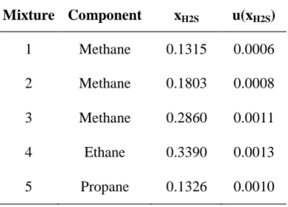
CO2 transport in the liquid-dense (vessels) and supercritical (pipelines) phases is more

advantageous than in the gaseous state due to the relatively high density with a relatively low viscosity of CO2 steams above the critical pressure (Figure 1.3).

Generally, captured gaseous CO2 is compressed to a pressure up to 8 MPa in order to

avoid two-phase regime during the transportation [2]. The reason behind is that the critical pressure of CO2 is 7.38 MPa [10]. Therefore, above this pressure it is guaranteed

that there will be no phase change with temperature variation along the pipeline. However, the presence of impurities will affect the critical pressure of the CO2-rich

steam (Figure 1.4), leading to the coexistence of liquid and vapour phases. Thus, the specification for composition of CO2 steam is an important requirement in the design of

pipelines (Table 1.1).

Table 1.1. Example of composition specifications [11].

Component Contain Limitation

Carbon dioxide > 95% of CO2

Water < 500 ppm* Solubility limit of water in CO2

Oxygen < 4 vol %

(< 1000 ppm* EOR applications)

Total content of non-condensable gases (O2, CH4, N2, Ar and H2)

should not exceed 4 vol%

Nitrogen < 4 vol %

Hydrocarbons < 4 vol %

Hydrogen < 4 vol %

Argon < 4 vol %

Hydrogen sulphide < 200 ppm*

Health and safety considerations Carbon monoxide < 2000 ppm*

Sulphur oxides < 100 ppm*

Nitrogen oxides < 100 ppm*

* Parts per million by weigh

Elevated water and hydrogen sulphide contents cause much higher corrosion rates, and in the case of water might also form hydrates [2]. The range of pressures of a CO2 steam

to ensure a safe and cost-effective transport is defined by the ambient temperature range, the impurities and the condition of single dense phase operation. For example, the operating pressure range of the existing CO2 pipelines in the U.S. goes from 8.6 to

(36)

1 3 5 7 9 260 270 280 290 300 310 P / M P a T / K

Figure 1.4. CO2 saturation line (solid line) and predicted P-T envelop of two CO2-rich mixtures

(dashed lines). Symbols: experimental critical points of (●) pure CO2, (■) mixture 1 (94% CO2, 3%

O2 and 3% Ar) and (▲) mixture 2 (92% CO2, 3% O2 and 5% SO2) [13].

1.2.3 Storage

In the context of depleted hydrocarbon reservoirs, CO2 geological storage is associated

with enhanced oil recovery (CO2 EOR). The oil and gas industry has come to call the

phases of the production as Primary, Secondary and Tertiary. During the Primary Production Phase, oil and gas are produced by the pent-up energy of the confined fluids in the reservoir and when the pore pressure is depleted, “artificial lift” is used to increase the flow from the production well. At the end of this phase, sometimes up to 80-90% of the original oil in place (OOIP) is still in the reservoir. The Secondary Production Phase consists of water injection in order to repressurise the formation; therefore, new injection wells are drilled. Fresh water is not used and the produced water is recirculated into the ground again. It is often that, even after the second phase, 50-70% of OOIP remains in the reservoir. The CO2 enhanced oil recovery (EOR) is

used during the Tertiary Production Phase. Injecting almost pure CO2 (<5% of

impurities), oil viscosity and surface tension between the fluid and the reservoir rock are reduced, leading to the CO2 sweeping up the oil from the injector to the producer well

[14].

Mineral sediments (e.g. sand, clay) and other particles (e.g. crushed shells, precipitated carbonates) were deposited over millions of years, and then they were pressurized and cemented as more materials have been piled on, forming the called sedimentary rocks.

(37)

The CO2 is injected in these rocks at depths of around 1000 meters or more, to ensure

that it does not escape and also to have enough pressure (due to the overburden) to maintain CO2 as critical fluid. These sedimentary rocks (e.g. sandstone and limestone)

are permeable, with porosities between 10% and 30%, which allows fluid to flow through them. The void-spaces are full of water or oil and gas, depending on if it is a reservoir or an aquifer. Both reservoir and aquifer need to be confined by a cap rock, an impermeable rock which prevents upwards fluid migration as a result of structural or stratigraphic trapping.

Figure 1.5: CO2 trapping mechanism [2].

CO2 storage follows four different trapping mechanisms. These trapping processes take

place over many years at different rates from days to years to thousands of years, but, in general, the storage security increases with time since the end of the injection, due to the appearance of a more stable mechanism (Figure 1.5). According to a chronology succession, the geological storage mechanisms are [15]:

 Structural/stratigraphic trapping. CO2 is confined by impermeable rocks (e.g.

shales). Once CO2-rich phase is injected, it percolates through the porous rock until

the top of the formation where is trapped. This is the most dominant of the trapping mechanisms.

 Residual/capillary trapping. CO2 is kept in pores. When the CO2 moves through the

(38)

surface tension between injected CO2-rich phase and the other phases contained in

the pores. This is often the mechanism which holds oil for millions of years.

 Solubility trapping. CO2 is dissolved in underground water. This phase of the

trapping process involves the CO2 dissolution into the salt water (or brines) already

present in the porous rock. This phenomenon can be probably attributed to the fact that water containing CO2 is denser and sinks to the bottom of the formation over

time.

 Mineral trapping. CO2 crystallizes into carbonate rock. Dissolved CO2 forms weak

carbonic acid, which can react with the minerals present in the surrounding rock to form carbonate minerals. This is the most secure and final phase of trapping.

This research will, however, be focussed on neither stratigraphic nor mineral trapping, since the former just depends on the geology and morphology of the surrounding rock and the latter is a chemical process. From a thermodynamic point of view, capillarity and solubility trapping are processes which require predictive phase equilibria calculations of reservoir and rich-CO2 fluids. In this sense, the presence of impurities

will change the thermophysical properties, such as interfacial tension (IFT), capillary pressure and solubility.

1.3 Goals

Leaving aside the CCS aspects previously presented, which have been studied, there are still unanswered questions about carbon capture, transport and storage. The cost of investment and the cost of energy for capture, purification and storage of CO2-rich gas

flows, among others, are key engineering challenges that still require further investigation [16]. For example, from the technological point of view, a very important element is the transportation, mainly by pipelines, as the CO2 stream could contain other

gases like CH4, N2, O2, H2S, SO2, NOx and Ar. These impurities can change the

thermodynamic behaviour of the stream and cause a breakdown in the pipeline [17]. This implies that to economically optimize the process, CCS technology requires increasing the energy efficiency. From the approach of this work, it means describing with the highest precision the thermodynamic properties in order to define accurately the energy required for any process involved in CCS [18].

(39)

The main objective of the work developed in this thesis has been to study the phase equilibria of reservoir fluids and typical compounds of flue gases. To this end, it has been necessary to develop a thermodynamic model from an accurate equation of state (EoS) for CO2, hydrocarbons and other gases, such as N2, O2, H2S, Ar, etc. Several

EoSs are assessed to achieve this goal, by analysing the accuracy in their thermodynamic representation.

Besides studying phase equilibria, the second goal of this thesis has been to model the transport properties of CO2-rich systems, such as density, viscosity and interfacial

tension.

Another objective of this research has been to contribute with reliable experimental work: to study the vapour-liquid equilibria of one system relevant for the CCS projects which has not been investigated, to measure the density of hydrogen sulphide systems and to investigate the density and viscosity of a synthetic mixture of CO2 with high

level of impurities.

1.4 Thesis overview

In Chapter 2, the experimental work and procedure used in this research are explained and the measured data are presented. In Chapter 3, a description of the molecular forces and the definition of phase behaviour are presented. The concept of Equation of State (EoS) and the Statistical Associating Fluid Theory (SAFT) are also introduced in Chapter 3. A complete description of the model which is primarily used in this research, the SAFT-VR Mie EoS, is presented in Chapter 4. Additionally, in this chapter, a comparative study of vapour-liquid equilibria and density modelling with four different EoSs is presented. In Chapter 5 about transport properties, the viscosity and interfacial tension models are then described, as well as the results of modelling CO2-rich systems

concerning the transport properties. In Chapter 6, the experimental measurements presented in the Chapter 2 are then modelled and discussed. Finally, in Chapter 7, the main conclusions that can be extracted from the studies developed in this thesis are summarised and recommendations for future works are proposed.

(40)

(41)

CHAPTER 2: EXPERIMENTAL STUDY

This chapter aims to provide data interesting for the CCS. It is divided into two parts: first a literature review, where existing experimental data are analysed and systems showing a lack of experimental data (VLE and densities) are identified, then the experimental work done (experimental procedures, measurements and their uncertainties) during this thesis. Phase equilibrium data, density and viscosity of CO2 or

H2S systems have been measured. Data presented in this chapter will be used in the

following chapters to validate the investigated models.

2.1 Introduction

In the context of the Carbon Capture and Storage, the compounds of interest are the one present in reservoir fluids and typical flue gas. Seven gases (CO2, N2, O2, Ar, H2S, CO

and SO2), twenty alkanes (between methane and nC32) and two aromatics (benzene and

toluene) have been chosen to validate the model. A summary of the VLE and density data available in the literature for the studied binary mixtures is presented in Table 2.1.

Systems studied experimentally have been chosen because of one of these criteria: lack of experimental data, extension of the conditions range and continuity in the work of our research centres. First, vapour-liquid equilibrium (VLE) of the Ar- H2S binary

system has been studied. No data have been found in the literature for this system and both H2S and Ar are components present in reservoirs (traces of Ar in natural gases) and

flue gas steams. Second, densities of three systems of CH4 + H2S have been measured in

order to extend the range of data to lower temperatures (253K). Densities of a C2H6 +

H2S and a C3H8 + H2S systems have also been measured complementing the work of

Rivollet [20,21,22] at the laboratories of the CTP Mines-ParisTech. Third, in the framework of the joint industrial project (JIP) entitled “Impact of Common Impurities on Carbon Dioxide Capture, Transport and Storage” [23], the densities of a ternary system of CO2-CH4-H2S have been measured. Also as part of this JIP and continuing

the work of Nazeri [24] at the labs of the IPE in the Heriot-Watt university, the density and viscosity of a multicomponent CO2-rich synthetic mixture have been studied.