OATAO is an open access repository that collects the work of Toulouse
researchers and makes it freely available over the web where possible
Any correspondence concerning this service should be sent
to the repository administrator:
tech-oatao@listes-diff.inp-toulouse.fr
This is an author’s version published in: http://oatao.univ-toulouse.fr/26562
To cite this version:
Oberlin, Thomas
and Meignen, Sylvain
and Perrier, Valerie
Second-Order synchrosqueezing transform or invertible
reassignment? Towards ideal time-frequency representations.
(2015) IEEE Transactions on Signal Processing, 63 (5). 1335-1344.
ISSN 1053-587X
Official URL:
Second-Order Synchrosqueezing Transform
or Invertible Reassignment? Towards Ideal
Time-Frequency Representations
Thomas Oberlin, Sylvain Meignen, and Valérie Perrier
Abstract—This paper considers the analysis of multicomponent
signals, deÞned as superpositions of real or complex modu-lated waves. It introduces two new post-transformations for the short-time Fourier transform that achieve a compact time-fre-quency representation while allowing for the separation and the reconstruction of the modes. These two new transformations thus beneÞt from both the synchrosqueezing transform (which allows for reconstruction) and the reassignment method (which achieves a compact time-frequency representation). Numerical experi-ments on real and synthetic signals demonstrate the efÞciency of these new transformations, and illustrate their differences.
Index Terms—Time-frequency, reassignment, synchrosqueez
-ing, AM/FM, multicomponent signals.
I. INTRODUCTION
M
OST real signals can be accurately modeled as su-perpositions of locally bandlimited, amplitude and frequency-modulated (AM-FM) waves. Containing several modes they are often called multicomponent signals (MCS). Many approaches have been built to decompose these signals into their constituent modes either in time-frequency (TF) domain, like the synchrosqueezing transform [1], or in time domain, as for instance the empirical mode decomposition (EMD) [2], [3]. Yet, very few results on the accuracy of the mode retrieval are available. In this regard, a new approxima-tion result on the retrieval of weakly modulated modes of an MCS has been shown using the synchrosqueezing transform (SST) [4]. This major result inspired new developments of syn-chrosqueezing or reassignment methods, and more generally of local TF analysis and synthesis techniques [5]–[7]. To obtain such a result, very strong assumptions were made on the modes making up the signal among which the most limiting one is the weak modulation hypothesis on the modes.T. Oberlin is with IRIT/INP-ENSEEIHT, University of Toulouse, Toulouse 31000, France (e-mail: thomas.oberlin@enseeiht.fr).
S. Meignen and V. Perrier are with the Jean Kuntzmann Laboratory, Uni-versity of Grenoble-Alpes, and CNRS, Grenoble 38041, France (e-mail: syl-vain.meignen@imag.fr; valerie.perrier@imag.fr).
Indeed, most MCS contain strongly frequency modulated modes, as for instance chirps involved in radar [8], speech processing [9], or gravitational waves [10]. Although many TF transforms such as quadratic distributions [11], [12] or the reassignment method (RM) [13]–[16] manage to accurately represent these kinds of signals, they do not allow for mode separation and reconstruction. Recently, some work has been done on how to deal with high FM with SST. For instance, in [16], a two-steps algorithm is used, which Þrst computes SST, estimates the FM, and Þnally recomputes SST on the demodulated mode. In the same spirit, an iterative procedure is proposed in [17], where at each iteration a SST is computed at a Þner resolution. A different and earlier attempt [18] consisted in building an invertible extension of RM. Unfortunately, the proposed reconstruction was only an approximation, valid for Gaussian windows with a small temporal width. We will see that contrary to [16], [17], our approach is one-step: it only consists in computing a reassignment map and then rearranging the coefÞcients of the STFT according to that map following this idea of the original synchrosqueezing or reassignment methods. Thus, it can be seen as an extension of [18], with ad-ditional theoretical results for representation and reconstruction of linear chirps.
The aim of this paper is indeed to extend SST to MCS con-taining strongly frequency modulated modes by generalizing SST in two different ways. The Þrst attempt is inspired by RM, which is known to optimally sharpen the TF representation of a linear chirp. However, in the original RM the sharpened repre-sentation obtained from the spectrogram did not allow for mode retrieval. We will see that by fully exploiting the information contained in the so-called shape reassignment vector, one can derive a new generation of SST that provides a sharpened TF representation as good as the one given by RM, while enabling exact retrieval of linear chirps. Our second approach relies on a second-order local estimate of the instantaneous frequency, which is used to improve modes localization and reconstruction using SST.
The outline of the paper is as follows: in Section II, we recall important notations that are subsequently used in the paper and we introduce the concept of weakly modulated modes. We then deÞne SST and RM in Section III, putting the emphasis on the differences in terms of reconstruction and representation. Then, Section IV is devoted to the presentation of the new extensions of SST. Section V Þnally delivers numerical results on both syn-thetic and real data, comparing the proposed methods with stan-dard SST and RM.
II. TIME-FREQUENCY ANALYSIS OF
MULTICOMPONENTSIGNALS
A. Short-Time Fourier Transform
DeÞnition II.1: The Fourier transform of a function
is deÞned by
For a given represents the part of that oscillates at fre-quency on the whole time domain. The need for time-localized frequency descriptors leads to the following deÞnition:
DeÞnition II.2: Let a real-valued and even func-tion, with unit norm. The short-time Fourier transform (STFT) of , with respect to the window , is deÞned by
(1) The representation of the positive quantity in the TF plane is called the spectrogram of . Without ambiguity, will be denoted by .
Remark: The usual deÞnition of STFT differs from (1) by
a factor and considers the conjugate of . Also, as we assume to be real-valued, we do not need the conjugate in (1).
It is well known from the properties of the Fourier transform that a well-localized TF representation requires a window well localized both in time and frequency. We shall then mention that STFT is invertible on using either of the following formulae:
(2) (3) Note that (3) is valid only if is non-zero and continuous at 0. If the signal is analytic (i.e., then the integral domain for is restricted to .
B. MCS and Ridges
DeÞnition II.3: An AM-FM mode is an oscillating function
, with and positive and slow-varying. is called the instantaneous amplitude of at time being its instantaneous frequency. Note that the slow-varying condition is not quantiÞed being model-dependent as explained later. Thanks to that condition, a Þrst order expansion of the phase combined with a zeroth order expansion of the amplitude lead to the approximation, for close to a Þxed time :
The STFT of mode is then approximated by [4], [19]: (4) This shows that the STFT of an AM-FM mode is non-zero on a TF strip, centered on the ridge corresponding to its instan-taneous frequency and deÞned by . The width of this
strip depends on that of the support of . Let us now deÞne MCS which are superpositions of AM-FM modes.
DeÞnition II.4: A MCS reads
(5) where the modes satisfy .
In order to retrieve each mode from the STFT of , we assume that the modes occupy non-overlapping regions in the TF plane. Considering (4) and assuming is compactly supported, this requires that the distance between two ridges is always larger than the width of the frequency support of window [4], [19]. This will be detailed in Section III.C. Note that this separation condition is of a linear type for STFT and can be adapted to non-compactly supported, but rapidly decreasing windows in the Fourier domain (e.g., Gaussian windows).
III. SYNCHROSQUEEZING ANDREASSIGNMENT IN ANUTSHELL
The so-called reassignment method (RM) [13], [14] is a gen-eral way to sharpen a TF representation towards its ideal TF
representation which corresponds for MCS given by deÞnition
II.4 to:
(6) being equal to 1 or 2 depending on whether a linear or a quadratic representation is used (e.g., for the spectrogram and for STFT). Note that keeps the phase informa-tion, which enables the reconstruction of the mode in the case of linear representations . Quadratic representations often remove the phase, and use the amplitude of instead of .
A. Reassignment of the Spectrogram
RM presented here in the spectrogram context consists of the computation of so-called reassignment operators:
(7) where can be viewed as an approximation of the instan-taneous frequency and as the group delay. Then, the reas-signment step aims to retrieve the ideal TF representation by moving the coefÞcients of the spectrogram according to the map
, which reads:
B. STFT-Based SST
The aim of SST based on STFT (FSST), introduced in [1] in the CWT context, is to retrieve the ideal TF representation, i.e., with , from its STFT. Following [1], the authors in
[20], [19] proposed to neglect operator , and to reassign only the complex coefÞcients according to the map
, which reads:
(8) Knowing , the th mode can then be retrieved by considering: (9) as explained in more details in Section III.C. In a nutshell, FSST reassigns the information in the TF plane and then makes use of this sharpened representation to recover the modes. The ratio-nale behind (8) and (9) is the reconstruction formula (3), where the integration is restricted to a mode-related domain instead of . This enables to retrieve the modes which was not possible with RM based on the spectrogram, but the TF representation is unfortunately less sharp as soon as the frequency modulation is not negligible. This difference between FSST and RM is further illustrated in Section III.D.
C. Perfect Localization and Reconstruction
We now recall the main properties of FSST and RM in terms of TF localization and mode reconstruction for FSST. We Þrst highlight for what type of signals they actually lead to the ideal TF representation and then consider a more general case.
1) Synchrosqueezing for Perturbations of Pure Waves: One
can show that actually matches the instantaneous frequency only for a pure tone . In this case, FSST provides the ideal TF representation given by (6). More interesting is the study of the behavior of FSST on perturbations of pure waves, i.e., containing “small” amplitude and frequency mod-ulations. This analysis was pioneered in [4] for the SST based on wavelets, and was adapted for FSST in [19]. It starts by deÞning precisely a MCS, originally referred to as ‘intrinsic mode type function” [4].
DeÞnition III.1: Let and . A MCS of type (5) is in if:
• for all satisÞes:
and for all and .
• the s are separated with resolution i.e., for all and for all ,
One can then deÞne the synchrosqueezing operator, using a function , the space of compactly supported smooth functions, such that , a threshold and an accuracy parameter :
and Þnally state the main result.
Theorem III.1: Let and . Consider a window , the space of smooth functions with fast decaying derivatives, such that . Then, if is small enough,
• only if there exists such
that .
• For all and all pair such that , one has
• For all there exists a constant such that for all ,
(10) The proof of this result is available in [19]. Equation (10) shows that the synchrosqueezing operator has to be summed up around the ridge, the width of the interval being . As in prac-tice is not known, one chooses a parameter instead. There-fore we end up with reconstruction formula (9) for mode . Note that a similar approximation result was stated before in [20], but with stronger (global) assumptions on the mode sepa-ration , instead of the local one in DeÞnition III.1.
To summarize, the FSST of a MCS offers both good localiza-tion and reconstruclocaliza-tion if two restrictive condilocaliza-tions are satisÞed: • the frequency separation , which is however necessary to uniquely deÞne the decomposition, • and the low-modulation assumption , that we
want to relax in the sequel.
2) Reassignment of Perturbations of Linear Chirps: It was
shown in [14] that the reassignment operators perfectly localize linear chirps, i.e., modes with a linear instantaneous frequency and constant amplitude. More precisely, one has the following result [14].
Theorem III.2: Consider a pure linear chirp
, where is a polynomial of degree 2 and . Then, whenever the reassignment operators are deÞned one has
.
Proof: In spite this result is available in [14], we recall its
main lines for the sake of introducing some notation that will be useful in the sequel.
Let us consider a linear chirp with . For such signal, one has for each and :
(11) The STFT then writes
with . We can now derive the expression of the reas-signment operator :
we Þnally get
(12) Note that the nature of function is unknown, although in the case of a Gaussian window , one can show that it is linear [7], [21]. But one can remark that it is still a smooth function provided is smooth and has fast decay.
Regarding the local time delay deÞned in RM, in the case of a linear chirp , we can write
(13) which again uses auxiliary function . Remembering that
, we get from (12) and (13) that:
(14) which means is an exact estimate of the instantaneous frequency , but at a shifted time location given by .
As the operators are local, this suggests that whenever the instantaneous frequency is quasi-linear and the amplitude slow-varying, the reassignment provides an accurate approximation of the ideal TF representation.
D. Illustrations
To illustrate the differences between FSST and RM, we use two synthetic test signals throughout this paper. One (signal 1) is made of low-order polynomial chirps, that behave locally as linear chirps, and the other one (signal 2) contains strongly nonlinear sinusoidal frequency modulations and singularities (points where ). Fig. 1 displays FSST and RM for these signals. Note that wherever the slope of the ridge is strong, RM gives a more concentrated representation than FSST.
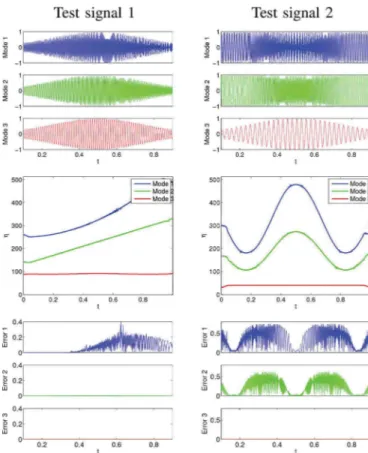
To illustrate the speciÞcity of FSST regarding invertibility, we display on Fig. 2 the reconstruction process of each test signals from FSST. To compute an estimation of the ridges , knowing the number of modes, we use the algo-rithm introduced in [22] and used in [23] or [7], which computes a local minimum of the functional
(15) where is an estimator of the ridge , and and are two positive parameters tuning the level of regularization. Other ridge detectors such as the one developed in [24] may of course be used instead but this is beyond the scope of the present paper.
Looking at the results of Fig. 2, it is worth noting that the quality of the reconstruction of a mode is highly dependent on its modulation. For instance mode 2 and 3 of signal 1 are properly
Fig. 1. Illustration of FSST and RM for test signal 1 (left) and 2 (right). From top to bottom: the spectrogram, FSST and RM.
retrieved but so is not mode 3 since it contains stronger modu-lations. Our goal is thus, in what follows, to improve mode re-construction based on FSST when the modes are strongly mod-ulated.
IV. TOWARDS ASECOND-ORDERFSST
Recalling that FSST was designed to process superpositions of perturbed pure waves, by second order FSST we mean that we want to adapt FSST to superpositions of perturbed linear chirps. This should enable us to obtain an invertible sharpened TF representation of the same quality as the one provided by RM. We are going to consider an approximation of the second derivative of the phase of the modes which we will subsequently use to build our extensions of FSST.
A. Local Instantaneous Modulation
This approximation requires the computation of second-order derivatives of the phase of the STFT, that have been already used to improve the reassignment method [6]. This is denoted by and deÞned as follows:
DeÞnition IV.1: Let be in . Its modulation operator is deÞned wherever and
by:
(16) Operator can be seen as some variation measure of the reassignment vector. Note that there are many other possible choices for this local estimate of the frequency modulation. In particular, we could also use , which amounts
Fig. 2. Illustration of mode retrieval based on FSST on test-signals 1 (left) and 2 (right). From top to bottom: the three modes making up the test-signals, their SST with the estimated ridges superimposed, and the reconstruction error. SNR after reconstruction for modes 1, 2 and 3 equals 14, 51 and 70 dB for test-signal 1, and 5, 7 and 70 dB for test-signal 2, respectively. We use in the reconstruction (see (9)), and for the ridge extraction (see (15)).
to adding a real (resp. imaginary) part in the numerator (resp. denominator) of (16). We keep deÞnition (16) since it appears to be more stable numerically. The following result shows that the local operator perfectly estimates the frequency modulation for a linear chirp.
Proposition IV.1: If is a Gaussian-mod-ulated linear chirp (i.e., both real-valued functions and are quadratic), then wherever is deÞned one has
Proof: Function is obviously differentiable, and its derivative reads
If satisÞes the following simple differential equa-tion:
(17)
where is an afÞne complex-valued function, since functions and are quadratic. Thus, there exists complex numbers
and such that . Let us now differentiate the STFT with respect to :
Dividing by and differentiating with respect to gives
Recalling that (17), we Þnally get the result. Let us Þnally give a convenient formula to compute through simple element-wise operations on different STFT’s.
Proposition IV.2: Operator can be computed according to: (18) where and are the STFT of with windows and
.
Proof: To enlighten the notation we will write instead of . Operator writes:
(19) For any signal , we have
We also have
Combining these expressions Þnally gives (18).
B. Vertical Second-Order Synchrosqueezing
Equation (12) clearly shows that does not hold as soon as . We propose a Þrst way to deal with the non-negligible modulation . Let
be a linear chirp with constant FM . Equations (12) and (13) show that for any time ,
which means that the Þrst order Taylor expansion of can be written in terms of the Þrst reassignment and frequency mod-ulation operators. Using locally the chirp approximation for a
given signal , one can now improve the estimation of the in-stantaneous frequency as follows:
DeÞnition IV.2: Let , we deÞne the second-order
instantaneous frequency estimator of by:
The vertical second-order synchrosqueezing (VSST) then consists in replacing by in standard SST:
Since the coefÞcients are only moved vertically, the reconstruc-tion is still achievable by summing up the FSST coefÞcients in the vicinity of the ridge replacing in (9) by . Moreover, as all the operators are local, VSST should remain efÞcient for small perturbations of linear chirps. This will be further studied numerically in the next section.
C. Slanted Synchrosqueezing
An alternative way to modify FSST to take into account FM consists in moving the coefÞcients according to the reassign-ment vector Þeld while keeping the phase information so as to allow signal reconstruction. A Þrst attempt in this direction de-Þned the following complex reassigned transformation [18]:
Unfortunately, this deÞnition allowed for an approximative re-construction only for Gaussian windows, and resulted in non-negligible errors as demonstrated by numerical results.
Let us now propose an alternative reassignment technique computing the phase-shift in a different way from [18] and that we will call oblique (slanted) synchrosqueezing (OSST). The starting point is to remark that the STFT of a linear chirp is in-variant by translations along the direction of the ridge
modulo a phase shift. Indeed, one can write, using (11) and ,
Instead of reassigning the real value as in RM, we propose to move the complex quantity
Contrary to VSST where one builds a Þrst order Taylor expan-sion of the derivative of the phase, OSST directly involves the
Fig. 3. Illustration of oblique synchrosqueezing (OSST).
phase-shift. For a linear chirp and when , one has so that one can then write:
This phase-modiÞed coefÞcients belong to the vertical line . Finally, summing up all the phase-shifted co-efÞcients along the frequency axis will provide an approxima-tion of at time .
The principle of OSST is illustrated on Fig. 3 the coefÞcients making up the dashed curve are phase-shifted while moved to point . To obtain an approximation of the signal , the phase of the coefÞcients are modiÞed in order to be equal to their projection on the dashed dotted line.
Let us now give a more formal deÞnition of OSST.
DeÞnition IV.3: Let , its oblique syn-chrosqueezing (OSST) is the function
An approximation of mode is then given by its OSST on the ridge, i.e.,
As for FSST and VSST, we would like OSST to remain ef-Þcient for perturbations of linear chirps, when the amplitude (resp. phase) is not exactly constant (resp. quadratic). Recall that for FSST and VSST, the strategy to handle such perturbations was to integrate the coefÞcients around the ridge using (9), so as to compensate for the error made by estimating the instan-taneous frequency by . However, in the case of OSST the coefÞcients are moved both in time and frequency, making this regularization impossible. We will see in the next section how this impacts the performance of the proposed technique.
V. NUMERICALRESULTS
To achieve a quantitative comparison between the different methods, we will reuse the test signals deÞned in Section III.D. Recall that test signal 1 is made of quasi-linear chirps that should be well dealt with by VSST or OSST, while test signal 2 con-tains stronger nonlinear frequency modulations as well as sin-gularities where vanishes, which makes the study of such signals more difÞcult. For the sake of simplicity, we focus on the representations based on STFT, but similar results could be obtained within the wavelet framework (see for instance [19] for a comparison). Note that in our simulations, we use 1024
Fig. 4. Test signals number 1 (left) and 2 (right). From top to bottom, magni-tude of FSST, OSST and VSST.
time samples and a Gaussian window with parameter , deÞned by .
On Fig. 4, FSST, VSST and OSST for both signals 1 and 2 are depicted. Comparing with Fig. 1, one notices that both VSST and OSST provide a nice TF representation, as sharp as RM. In the next subsections, we will compare more quantitatively the three methods in terms of the sharpness of the represen-tation (i.e., how many coefÞcients are signiÞcant at each time instant) and accuracy of mode reconstruction. We also numer-ically investigate the robustness to noise, and Þnally compare the methods on some real data.
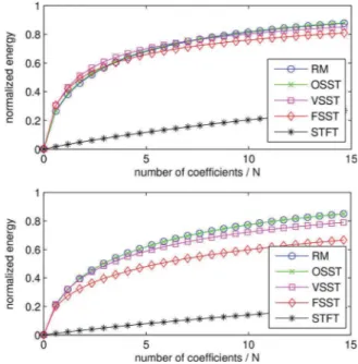
A. Quality of Representation
The main purpose of RM was to make TF representations more readable. Since this is somewhat subjective, we propose here to measure at each time step the amount of information contained in the coefÞcients with the largest amplitude. In this regard, one way to compare the different transformations is to compute the normalized energy associated with the Þrst co-efÞcients with the largest amplitude: the faster the growth of this energy towards 1, the sharper the representation. Fig. 5 dis-plays this normalized energy (i.e., the cumulative sum of the Þrst squared sorted coefÞcients over the sum of all the squared coefÞcients) for both test-signals and the Þve representations, namely STFT, RM, FSST, VSST and OSST. The Þrst remark is that both OSST and VSST behave similarly as RM for both test-signals. Indeed, the representation of test-signal 1 with each of these three methods is almost perfect, since one needs only 3 coefÞcients per time instant to recover the signal energy, which is consistent with the three modes making up the test-signal. Comparatively, the energy of FSST grows rapidly to reach a
Fig. 5. Normalized energy as a function of the number of coefÞcients for test-signal 1 (top) and 2 (bottom). Abscissa gives the number of coefÞcients over the size of the signal, i.e., the mean number of coefÞcients for each column of the TF plane.
Fig. 6. Normalized energy as a function of the number of coefÞcients for the noisy (0 dB) test-signal 1 (top) and 2 (bottom).
value around 80% and then stagnates which means the signal energy cannot be retrieved with a reasonable number of coef-Þcients. The results are similar but less sharp for the second test-signal, since it contains stronger nonlinear frequency mod-ulations.
In order to visualize the inßuence of noise, we carry out the same experiments when the test-signals are contaminated by white Gaussian noise (noise level 0 dB). The results displayed on Fig. 6 exhibit a slower increase of the energy since the coef-Þcients corresponding to noise are spread out in the whole TF plane. However, OSST, RM and VSST still behave better than FSST, even though VSST is slightly less competitive.
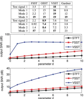
TABLE I
DIRECTRECONSTRUCTION FOREACHMETHOD,ANDBOTHTEST-SIGNALS. THEACCURACY OFMODERETRIEVALISEXPRESSED INSNR
Fig. 7. Reconstruction of the modes as a function of , which is proportional to the size of the interval of integration. The results are in SNR, for test signal 1 (top) and 2 (bottom).
B. Reconstruction of the Modes
The main advantage of FSST over RM is its invertibility. Let us recall that there are two possible reconstructions of the mode from FSST. The easiest one assumes is almost ideal, so that the whole information is concentrated on the ridge. The mode
at time is then estimated following
(20) FSST allows to achieve a more accurate reconstruction by using an integration around the ridge as a regularization step, according to formula (9). Provided is of the same order of magnitude as the perturbation deÞned in Theorem III.1, this formula ensures an asymptotically perfect reconstruction. It is important to recall here that this regularization process naturally applies to VSST but not to OSST.
We investigate here the accuracy of the reconstruction for each method starting with the reconstruction technique deÞned in (20). The results measuring the accuracy of mode reconstruc-tion in terms of SNR are displayed in Table I. We check that both OSST and VSST enable a good reconstruction of polynomial chirps (test-signal 1), whereas the quality of direct reconstruc-tion from FSST is very poor. Looking at the results for each mode, one observes that each method achieves a good recon-struction for mode 3 since it is not modulated, but that FSST is not adapted for modes 1 and 2 which contain stronger mod-ulations. The results are less convincing for test-signal 2: even if OSST and VSST improve the reconstruction compared with FSST, the accuracy is far from satisfactory. Indeed, as this signal contains strongly nonlinear frequency modulations, both OSST
Fig. 8. From top to bottom: the ridges estimated from FSST, those estimated from VSST, and the quality of reconstruction measured as a function of . We use again test signal 1 (left) and 2 (right).
and VSST fail to represent the modes as a perfect sharp curve in the TF plane, some information being spread out around the ridges. This result is in line with the simulation of Fig. 6 right, where on average 4 coefÞcients per time instant are needed to recover the most part of the energy.
By integrating FSST and VSST around the ridge, following (9), one can deÞnitely improve the reconstruction results. The results for such a reconstruction are displayed on Fig. 7. For each test-signal, the SNR of the reconstruction is computed with respect to parameter . This time we display the SNR associated with the reconstruction of the whole signal but considering the modes individually would lead to the same results. Fig. 7 shows that VSST allows for a quasi-perfect reconstruction from very few coefÞcients ( dB for ). Conversely, with FSST, even if one uses a large , i.e., many coefÞcients, one cannot retrieve the modes with a high accuracy. It is important to recall that such a computation cannot be carried out on OSST therefore this technique is not mentioned in the results of Fig. 7. We already saw that, in the noise-free case, the reconstruc-tion is all the better that parameter is large. This is obviously not true when the signal is contaminated by noise: must be large enough to take into account the signal coefÞcients, while remaining small enough so as not to include too much noise in the reconstruction. We illustrate this quantitatively by making the same experiments as for Fig. 7 but in the noisy case. Note that in this case, the estimation of the ridges using formula (15) is worsened due to the presence of noise. The results of the ridge estimation are depicted on Fig. 8, together with the reconstruc-tion accuracy, for both FSST and VSST and with a moderate noise level ( dB). While the ridge estimation can
Fig. 9. TF representations of a bat echolocation call. The representations are (from top to bottom) STFT, FSST, OSST and VSST. A zoom on strong modu-lations is displayed in the second column.
be successfully carried out on FSST and VSST for test-signal 1, only VSST gives a correct estimation for test-signal 2 since the latter contains stronger FMs. As a result, the reconstruction of test-signal 2 from FSST is not satisfactory. This study tells us that to take into account second order terms in the deÞnition of VSST not only improves the quality of mode reconstruction but also of ridge detection.
C. Illustration on Real Signals
We now illustrate the qualitative improvement of the two new transformations on real data. We start with considering a bat echolocation call, available at http://dsp.rice.edu/sites/dsp.rice. edu/Þles/software/batsignal.zip. Fig. 9 displays both VSST and OSST of this signal, and compare them with the spectrogram and FSST (parameter being set to 0.04 , with the duration of the signal). By zooming around a portion of one ridge, the improvement brought about these new methods in terms of the sharpness of the representation is undeniable. Note that the re-sult provided by FSST remains satisfactory since the frequency modulation is quite weak.
To better illustrate that improvement, we then considered a portion of a speech signal recorded at 44.1 kHz, with parameter set to 0.025 . Fig. 10 shows the corresponding TF repre-sentations associated with the four different methods, as well as a zoom on a modulated portion. For both VSST and OSST, the energy of the representation is almost perfectly concentrated along the ridges which is not the case with FSST. Note also that the representation given by OSST seems slightly better but if we were interested in reconstructing the modes, VSST would still behave better due to local frequency integration embodied by (9).
Fig. 10. TF representations of a speech signal. The representations are (from top to bottom) STFT, FSST, OSST and VSST. A zoom on a strongly modulated part is displayed on the second column.
VI. CONCLUSION
This paper introduced the vertical and oblique second-order synchrosqueezing transformations to circumvent the limitations of standard FSST and reassignment. We emphasized that OSST can be viewed as a complex version of the reassignment method, while VSST keeps the Þxed-time structure of the standard syn-chrosqueezing transform, allowing for a better reconstruction through a regularization step. We showed that both methods provide the ideal invertible representation in the case of a linear chirp, while remaining efÞcient on general multicomponent sig-nals containing strong frequency modulations. All the experi-ments suggest that OSST is slightly more competitive for the representation purpose, whereas VSST allows for a better re-construction.
Finally, note that both OSST and VSST can be extended readily to the wavelet setting. Further work should be devoted to the theoretical analysis of both methods for perturbations of linear chirps, as well as a deeper understanding of the inßu-ence of noise on the reassignment operators and on the ridge estimation.
REFERENCES
[1] I. Daubechies and S. Maes, “A nonlinear squeezing of the continuous wavelet transform based on auditory nerve models,” Wavelets Med.
Biol., pp. 527–546, 1996.
[2] N. E. Huang, Z. Shen, S. R. Long, M. C. Wu, H. H. Shih, Q. Zheng, N.-C. Yen, C. C. Tung, and H. H. Liu, “The empirical mode decompo-sition and the Hilbert spectrum for nonlinear and non-stationary time series analysis,” Proc. Roy. Soc. London A, Math., Phys. Eng. Sci., vol. 454, no. 1971, pp. 903–995, 1998.
[3] G. Rilling, P. Flandrin, and P. Goncalves et al., “On empirical mode decomposition and its algorithms,” in Proc. IEEE-EURASIP Workshop
Nonlinear Signal Image Process. (NSIP), 2003, vol. 3, pp. 8–11.
[4] I. Daubechies, J. Lu, and H.-T. Wu, “Synchrosqueezed wavelet trans-forms: an empirical mode decomposition-like tool,” Appl. Comput.
Harmon. Anal., vol. 30, no. 2, pp. 243–261, 2011.
[5] S. Meignen, T. Oberlin, and S. McLaughlin, “A new algorithm for multicomponent signals analysis based on synchrosqueezing: With an application to signal sampling and denoising,” IEEE Trans. Signal
Process., vol. 60, no. 11, pp. 5787–5798, 2012.
[6] F. Auger, E. Chassande-Mottin, and P. Flandrin, “Making reassign-ment adjustable: The Levenberg-Marquardt approach,” in Proc. IEEE
Int. Conf. Acoust., Speech, Signal Process. (ICASSP), 2012, pp.
3889–3892.
[7] F. Auger, P. Flandrin, Y. Lin, S. McLaughlin, S. Meignen, T. Oberlin, and H. Wu, “Time-frequency reassignment and synchrosqueezing: An overview,” IEEE Signal Process. Mag., vol. 30, no. 6, pp. 32–41, 2013. [8] M. Skolnik, Radar Handbook. New York, NY, USA: McGraw-Hill,
1970.
[9] J. W. Pitton, L. E. Atlas, and P. J. Loughlin, “Applications of posi-tive time-frequency distributions to speech processing,” IEEE Trans.
Speech Audio Process., vol. 2, no. 4, pp. 554–566, 1994.
[10] E. J. Candes, P. R. Charlton, and H. Helgason, “Detecting highly oscil-latory signals by chirplet path pursuit,” Appl. Comput. Harmon. Anal., vol. 24, no. 1, pp. 14–40, 2008.
[11] L. Cohen, Time-Frequency Analysis: Theory and Applications. Princeton, NJ, USA: Prentice-Hall, 1995.
[12] P. Flandrin, Time-Frequency/Time-Scale Analysis. New York, NY, USA: Academic, 1998, vol. 10.
[13] K. Kodera, C. De Villedary, and R. Gendrin, “A new method for the numerical analysis of non-stationary signals,” Phys. Earth Planet.
In-teriors, vol. 12, no. 2, pp. 142–150, 1976.
[14] F. Auger and P. Flandrin, “Improving the readability of time-fre-quency and time-scale representations by the reassignment method,”
IEEE Trans. Signal Process., vol. 43, no. 5, pp. 1068–1089, 1995.
[15] F. Auger, E. Chassande-Mottin, and P. Flandrin, “On phase-magni-tude relationships in the short-time Fourier transform,” IEEE Signal
Process. Lett., vol. 19, no. 5, pp. 267–270, 2012.
[16] C. Li and M. Liang, “A generalized synchrosqueezing transform for enhancing signal time-frequency representation,” Signal Process., vol. 92, no. 9, pp. 2264–2274, 2012.
[17] S. Wang, X. Chen, G. Cai, B. Chen, X. Li, and Z. He, “Matching de-modulation transform and synchrosqueezing in time-frequency anal-ysis,” IEEE Trans. Signal Process., vol. 62, no. 1, pp. 69–84, 2014. [18] T. Gardner and M. Magnasco, “Sparse time-frequency
representa-tions,” Proc. Nat. Acad. Sci., vol. 103, no. 16, pp. 6094–6099, 2006. [19] T. Oberlin, S. Meignen, and V. Perrier, “The Fourier-based
syn-chrosqueezing transform,” in Proc. 39th Int. Conf. Acoust., Speech,
Signal Process. (ICASSP), 2014, pp. 315–319.
[20] H.-T. Wu, “Adaptive analysis of complex data sets,” Ph.D. dissertation, Princeton Univ., Princeton, NJ, 2012.
[21] T. Oberlin, S. Meignen, and S. Mclaughlin, “Analysis of strongly modulated multicomponent signals with the short-time Fourier trans-form,” in Proc. 38th IEEE Int. Conf. Acoust., Speech, Signal Process.
(ICASSP), 2013, pp. 5358–5362.
[22] R. Carmona, W. Hwang, and B. Torresani, “Characterization of signals by the ridges of their wavelet transforms,” IEEE Trans. Signal Process., vol. 45, no. 10, pp. 2586–2590, 1997.
[23] G. Thakur, E. Brevdo, N. Fuþkar, and H.-T. Wu, “The syn-chrosqueezing algorithm for time-varying spectral analysis: robustness properties and new paleoclimate applications,” Signal Process., vol. 93, no. 5, pp. 1079–1094, 2013.
[24] R. Carmona, W. Hwang, and B. Torrésani, “Multiridge detection and time-frequency reconstruction,” IEEE Trans. Signal Process., vol. 47, no. 2, pp. 480–492, 1999.
Thomas Oberlin was born in Lyon, France, in 1988.
He received the M.S. degree in applied mathematics from Université Joseph Fourier, Grenoble, France, in 2010, as well as an engineer’s degree from Grenoble Institute of Technology. In 2013, he received the Ph.D. in applied mathematics from the University of Grenoble. In 2014, he was a post-doctoral fellow in signal processing and medical imaging at Inria Rennes, France. Since September 2014 he is an Assistant Professor with the INP Toulouse—EN-SEEIHT and the IRIT Laboratory, University of Toulouse, in Toulouse, France.
His research interests include adaptive and multiscale methods for signal and image processing, and in particular linear time-frequency analysis, syn-chrosqueezing, empirical mode decomposition. He is also interested in sparse regularization for inverse problems, and its applications in signal/image pro-cessing and medical imaging (e.g., in EEG).
Sylvain Meignen received his Ph.D. degree in
applied mathematics in 2001, and its “habilitation à Diriger Des Recherches” in 2011, both from the University of Grenoble, France. Since 2002, he has been an Assistant Professor with Grenoble INP. His research interests include nonlinear multiscale image and signal processing, time-frequency analysis (empirical mode decomposition, synchrosqueezing) and approximation theory. In 2010, he was a visitor at the GIPSA-Lab Grenoble and at the IDCOM of the university of Edinburgh, U.K., in 2011.
Valérie Perrier was born in Courbevoie, France.
She graduated from Ecole Normale Supérieure, St. Cloud, France, in 1987. She received the Agrégation of Mathematics, the Ph.D. degree in applied math-ematics from the University Paris VI, Paris, France, and the “Habilitation à Diriger des Recherches” from the University Paris XIII, Paris, France, in 1986, 1991 and 1996 respectively. In 1991, she joined the university Paris XIII, where she was Assistant Professor, and became Professor in 1997. In 1999, she moved to the engineering department Ensimag in Applied Mathematics and Computer Science, at Grenoble Institute of Technology, Grenoble, France. She is a member of the Laboratoire Jean Kuntzmann of the university of Grenoble, in charge of the research group “Geometric Modeling and Multiresolution for Images”. Her research interests include the use of wavelets in numerical simulations of partial differential equations, and multiscale methods for signal or image processing.
Dr. Perrier was awarded the 2003 Blaise Pascal Prize in applied mathematics from the French Academy of Sciences.