Modélisation d'un robot manipulateur en vue de la commande robuste en force utilisé en soudage FSW

(1)

HAL Id: tel-01305951

https://pastel.archives-ouvertes.fr/tel-01305951

Submitted on 22 Apr 2016

HAL is a multi-disciplinary open access

archive for the deposit and dissemination of sci-entific research documents, whether they are pub-lished or not. The documents may come from teaching and research institutions in France or abroad, or from public or private research centers.

L’archive ouverte pluridisciplinaire HAL, est destinée au dépôt et à la diffusion de documents scientifiques de niveau recherche, publiés ou non, émanant des établissements d’enseignement et de recherche français ou étrangers, des laboratoires publics ou privés.

Modélisation d’un robot manipulateur en vue de la

commande robuste en force utilisé en soudage FSW

Ke Wang

To cite this version:

Ke Wang. Modélisation d’un robot manipulateur en vue de la commande robuste en force utilisé en soudage FSW. Automatique / Robotique. Ecole nationale supérieure d’arts et métiers - ENSAM, 2016. Français. �NNT : 2016ENAM0003�. �tel-01305951�

(2)

N°: 2009 ENAM XXXX

Arts et Métiers ParisTech - Centre de Metz

2016-ENAM-0003

École doctorale n° 432 : Science des Métiers de l’Ingénieur

présentée et soutenue publiquement par

Ke WANG

le 28 janvier 2016

Robot manipulator modeling for robust force control

used in Friction Stir Welding (FSW)

~~~

Modélisation d’un robot manipulateur en vue de

la commande robuste en force utilisé en soudage FSW

Doctorat ParisTech

T H È S E

pour obtenir le grade de docteur délivré par

l’École Nationale Supérieure d'Arts et Métiers

Spécialité “ Automatique ”

Directeur de thèse : Gabriel ABBA

Co-encadrement de la thèse : François LEONARD

T

H

È

S

E

Jury

M. Guillaume MOREL,Professeur, Université de Pierre et Marie Curie, Paris VI Président M. Wolfgang SEEMANN,Professeur, Karlsruher Institute of Technology Rapporteur

M. Stéphane CARO,Chargé de recherche, IRCCyN, CNRS Rapporteur

M. Gabriel ABBA,Professeur, LCFC, Université de Lorraine Examinateur M. François LEONARD,Maître de conférences, LCFC, Université de Lorraine Examinateur

(3)

(4)

CONTENTS

Acknowledgements

I would like to acknowledge everyone who has helped me with my doctoral studies in any kind of way throughout the past three years.

First and foremost, I would like to express my sincere gratitude to my thesis supervisor Dr. Gabriel Abba for providing me with the excellent opportunity to achieve this work. I am really grateful for his patient and continuous guidance, tremendous support and encouragement with my scientiﬁc research and professional development. His wisdom, enthusiasm and friendly attitude have inspired me to try my best to overcome any diﬃculty of my work. With the help of his extensive knowledge and countless suggestions, I have learned a great deal of things both for the research and life. I am also grateful for his invaluable help in proofreading the manuscript and assisting me in preparing my doctoral dissertation defense.

I am also extremely grateful to my co-supervisor Dr. François Léonard for af-fording me technical guidance, generous support, flexible and valuable supervising time as well as his admirable patience and strong confidence on me. He has always been supportive and has provided me scientific knowledge and advice, insightful dis-cussions and helpful suggestions about my research. He has always encouraged me to think more independently and to get over the various obstacles. I have also ap-preciated the timely help that he has given to me, even in his vacation time, and the immense assistance in proofreading my manuscript and preparing my thesis defense. I would also like to thank all the members of my PhD thesis committee: Dr. Guillaume Morel, Dr. Wolfgang Seemann, Dr. Stéphane Caro and Mr. Aurélien Robineau for their support, encouragement, insightful questions and constructive suggestions. It is my great honor to have such a high level jury for my PhD defense. I want to give my special thanks to Dr. Wolfgang Seemann and Dr. Stéphane Caro for spending their precious time on reviewing my manuscript carefully and giving back their insightful comments and constructive advice to improve the quality of my thesis. Dr. Guillaume Morel has chaired the doctoral thesis defense and has given me some helpful comments on my research which inspired me a lot. I am also honored to be able to invite the FSW expert Mr. Aurélien Robineau to participate in my thesis defense and he has also given me a lot of valuable suggestions. I am really grateful for the inestimable contributions of all these jury members.

I would like to acknowledge and extend my appreciation to the colleagues and friends in the LCFC: Patrick Martin, Régis Bigot, Laurant Langlois, Sandra Chevret, Jean-yves Dantan, Ali Siadat, Naﬁssa Lakbakbi Elyaaqoubi, Alain Etienne, Eric Becker, Stéphanie Schiappa, Véronique Ernest, Zakaria Allam, Simon Jung, Flo-rian Baratto, Renaud Gimenez, Mathieu Hobon, Olivier Gyss, Damien Chevalier, Bruno Kaici, Thanh Hung Nguyen, Catalina Gutierrez, François Cristofari, Phillipe

(9)

CONTENTS

Mayer, Fawzia Dardouri, Maryam Zouhri, Jinna Qin, Guochao Gu, Fan Li, Qing Xia, Peng Wang, Zhicheng Huang, Haitao Tian, Jianjie Zhang, Zhongkai Chen and all others who have also contributed to my advancement throughout my doctoral studies. I want to thank everyone in the laboratory for the inspiring environment and friendly atmosphere they are creating and for all the fun we have had together in the past several years. I am particularly grateful to Maryam Zouhri for her precious friendship, warm care and heartfelt support.

My cordial and sincere thanks go to all my Chinese friends with whom I have shared the wonderful and amazing time in Metz. Special thanks to Jinna Qin, Guochao Gu and Zhongkai Chen for assisting me to adapt to the life in France, and Jinna Qin has helped me a lot both for the research work and daily life. I also want to thank Fan Li, Qing Xia, Peng Wang, Zhicheng Huang, Haitao Tian, Jianjie Zhang, Xianqiong Zhao and Da Li for taking photos during my oral presentation and for preparing the delicious buﬀet after my doctoral defense. I love all my dear Chinese friends in Metz and I appreciate the pure and precious friendship between us which is the most valuable asset of my life and will not be forgotten forever.

I also owe a special debt of gratitude to all of the staﬀ at ENSAM Metz and the doctoral school in Paris for giving me the immense help and generous support throughout my studies. Special thanks should go to the administrative crew of my laboratory: Stéphanie Schiappa and Véronique Ernest for their admirable patience and countless help in my research work. In addition, I am also indebted to the administrative personnel of the doctoral school: Florence Dumard, Claude Roy and the director Anne Bouteville for their timely assistance and warm encouragement.

The French National Agency of Research (ANR) and the China Scholarship Council (CSC) are gratefully acknowledged for the research project funding (under the project ANR-2010-SEGI-003-01-COROUSSO) and the PhD scholarship for my daily life (reference number: 201206020028), without which I would not ﬁnish my doctoral study and would not obtain the PhD degree in France.

Last but not least, I would like to give the most heartfelt thanks to my family members: my parents Ruyi Wang and Zhuohui Ren; my wife Fang Liu; my grand-parents Daohai Wang, Zhongcai Li, Wenqi Ren, Xiuqi Zhao; my uncle Anyi Wang, my aunt Ping Li, my brother Fei Wang, my little sister Zeyu Wang and other rela-tives in my beloved motherland China. My parents have sacrificed their lives for me and provided me with unconditioned deep love, admirable patience, selfless support and endless encouragement, without which I would not get to this day to finish my PhD study. Apart from my parents, I am also indebted to my wife Fang Liu for her immense patience, support, encouragement and love that she is constantly giving me without a word of complaint. I am also really grateful to all other rela-tives and friends for providing me with invaluable help, support and encouragement unconditionally throughout my life.

(10)

List of Figures

1.1 Industrial robots from 1959 to 1974 [9] . . . 19

1.2 Industrial robots from 1974 to 1984 [9] . . . 20

1.3 Industrial robots from 1985 to present [9] . . . 21

1.4 Worldwide annual installations of industrial robots [12] . . . 22

1.5 Industrial robots launched by four diﬀerent companies . . . 22

1.6 The outline and ﬂow of information in this dissertation . . . 30

2.1 Position description of a point in space . . . 32

2.2 Position and orientation description of an object . . . 33

2.3 X-Y-Z ﬁxed angles . . . 34

2.4 Description of modiﬁed Denavit-Hartenberg convention . . . 35

2.5 Robot KUKA KR500-2MT . . . 36

2.6 Geometric description of the robot . . . 37

2.7 Schematic of the ﬂexible joint model . . . 47

2.8 Interface of the software SYMORO+ . . . 47

3.1 The function f and its inclusion function [f ] as well as minimal inclu-sion function [f ]∗ from X to Y (X and Y correspond to R2_{) . . . .} ₅₃

3.2 The schematic of generation of the symbolic robot dynamic model . . 55

3.3 Diagram of the simpliﬁcation algorithm process . . . 57

3.4 Flow chart of the simpliﬁcation program . . . 59

3.5 Histogram statistics of term norm ratio for M44 . . . 61

3.6 The tool position, joint angular position, velocity and acceleration along the identiﬁcation trajectory (test IS0811A) . . . 67

3.7 Comparison between original component of M (q) and simpliﬁed com-ponent of M s(q) along the identiﬁcation trajectory (I) . . . 69

3.8 Comparison between original component of M (q) and simpliﬁed com-ponent of M s(q) along the identiﬁcation trajectory (II) . . . . 70

3.9 Comparison between original component of H(q, ˙q) and simpliﬁed component of Hs(q, ˙q) along the identiﬁcation trajectory . . . . 71

3.10 Comparison between original torque T and simpliﬁed torque T s along the identiﬁcation trajectory . . . 71

3.11 The tool position, joint angular position, velocity and acceleration along the linear FSW trajectory (test IS1709J) . . . 72

3.12 Pareto diagram: choose the most appropriate proportional factors for simplifying the inertia matrix M (q) in the linear FSW case based on the criteria of accuracy and simplicity . . . 73

(11)

LIST OF FIGURES

3.13 Comparison between original component of M (q) and simpliﬁed

com-ponent of M s(q) along the linear FSW trajectory (I) . . . . 75

3.14 Comparison between original component of M (q) and simpliﬁed com-ponent of M s(q) along the linear FSW trajectory (II) . . . . 75

3.15 Comparison between original component of H(q, ˙q) and simpliﬁed component of Hs(q, ˙q) along the linear FSW trajectory . . . . 76

3.16 Comparison between original torque T and simpliﬁed torque T s along the linear FSW trajectory . . . 76

3.17 The tool position, joint angular position, velocity and acceleration along the circular FSW trajectory (test IS1006P) . . . 77

3.18 Comparison between original component of M (q) and simpliﬁed com-ponent of M s(q) along the circular FSW trajectory (I) . . . . 79

3.19 Comparison between original component of M (q) and simpliﬁed com-ponent of M s(q) along the circular FSW trajectory (II) . . . . 79

3.20 Comparison between original component of H(q, ˙q) and simpliﬁed component of Hs(q, ˙q) along the circular FSW trajectory . . . . 80

3.21 Comparison between original torque T and simpliﬁed torque T s along the circular FSW trajectory . . . 80

3.22 Measured currents of all the motors during the linear FSW process (test 1709J) . . . 82

3.23 External deformation compensation of KUKA robot [73] . . . 83

4.1 Schematic drawing of friction stir welding . . . 87

4.2 Friction stir welding experiment and its three main stages [2] . . . 88

4.3 Measurements of the forces and torque applied on the tool during the FSW process implemented by an instrumented MTS-ISTIR-10 Friction Stir Welder on 6000 aluminum alloy with a welding depth of 6 mm [111] . . . 89

4.4 Experimental setup: FSW system based on robot KUKA KR500-2MT (by courtesy of Institut de Soudure, Goin, France) . . . 91

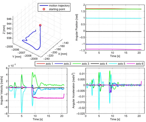
4.5 The desired welding trajectory in 3D space, measured (or calculated) joint angular position, velocity and acceleration of motor axes after the gear reduction along the welding trajectory (test IS1505I) . . . . 92

4.6 Measured currents of all the motors during the FSW test (test IS1505I) 93 4.7 Signal ﬂow schematic of the experimental testbed . . . 93

4.8 Diagram of the discrete observer for robot state estimation [73] . . . . 94

4.9 Diagram of data acquisition and processing for model identiﬁcation in the external observer-based test of KUKA robot . . . 95

4.10 Schematic of deﬁnition of the plunge depth dp . . . 96

4.11 Schematic of the ﬂexibility model in Cartesian space . . . 98

4.12 Comparison between ﬁltered and original measured axial force Fz during the FSW process (test IS1505I) . . . 100

4.13 Comparison between ﬁltered and calculated plunge depth dp and its derivative _dtddp (Method 1) . . . 101

4.14 Comparison between ﬁltered and calculated plunge depth dp and its derivative _dtddp (Method 2) . . . 102

(12)

LIST OF FIGURES

4.15 Comparison between ﬁltered and calculated plunge depth dp and its

derivative _dtddp (Method 3) . . . 103

4.16 Free-body diagram of simple lumped parameter model in z direction . 103 4.17 Comparison between ﬁltered and ﬁtted axial force Fz and generated error for Linear Model 1 . . . 107

4.18 Comparison between ﬁltered and ﬁtted axial force Fz and generated error for Linear Model 2 . . . 108

4.19 Comparison between ﬁltered and ﬁtted axial force Fz and generated error for Linear Model 3 . . . 108

4.20 Histogram of error and estimated Gaussian for Linear Model 1 with data ﬁltering . . . 109

4.23 Comparison between ﬁltered and ﬁtted axial force Fz and generated error for the nonlinear model . . . 113

4.24 Histogram of error and estimated Gaussian for the nonlinear model with data ﬁltering . . . 113

5.1 Inner position/outer force control scheme for industrial robot KUKA 119 5.2 System modeling in Cartesian space . . . 120

5.3 Time history of model parameters during circular FSW process (test IS1006P) . . . 123

5.4 Measured and ﬁtted displacements in x direction . . . 125

5.5 Measured and ﬁtted displacements in y direction . . . 125

5.6 Measured and ﬁtted displacements in z direction . . . 126

5.7 Bode diagram of three third-order transfer function models . . . 126

5.8 Measured and ﬁtted displacements in x direnciton . . . 127

5.9 Measured and ﬁtted displacements in y direction . . . 127

5.10 Measured and ﬁtted displacements in z direnciton . . . 127

5.11 Bode diagram of three kinds of models in z direction . . . 127

5.12 Block diagram of the axial force control system . . . 128

5.13 Nichols chart of the the open-loop transfer function excluding the rest part of force controller to be designed G∗_{F C}(s) (Phase-lead-lag case) . 132 5.14 Bode diagram of three force controllers . . . 135

5.15 Bode diagram of the open loop systems with three force controllers . 135 5.16 Schematic diagram of the position control of KUKA robot for FSW process (without the force control) . . . 136

5.17 Diagram of the continuous-time joint motion controller of the simulator139 5.18 Diagram of the discrete-time joint motion controller of the simulator . 140 5.19 Diagram of the main models in the simulator . . . 142

5.20 Three-dimensional model of robot KUKA in the FSW process . . . . 142

5.21 Schematic diagram of the simulator in Matlab/Simulink environment 143 5.22 Comparison of the axial forces during the simulations with three dif-ferent force controllers . . . 145

(13)

LIST OF FIGURES

5.23 Desired tool velocity in Cartesian space used in the simulation . . . . 145 5.24 Comparison of the desired tool position and the actual tool position

in 3D space during the simulation with only force control in z direction146 5.25 Comparison of the desired tool position and the actual tool position

in X-Y plane during the simulation with only force control in z direction146 5.26 Comparison of the desired tool position and the actual tool position

in X-Z plane during the simulation with only force control in z direction147 5.27 Measured axial force during friction stir welding process (test IS1709J:

Ω = 1100 tr/min, v = 400 mm/min, welding depth 6 mm, material

Al6082) . . . 148

5.28 Spectrum of the axial force in FSW process (test IS1709J) . . . 148 5.29 Welded workpiece after the FSW process (test IS1709J) . . . 149 5.30 Measured and ﬁtted z coordinates of the weld surface and

correspond-ing x coordinates (test 1709J, z coordinates denotes the height of weld surface and x coordinated denotes the position along welding direction)150 5.31 Height variations of the surface of welded workpiece ∆h and

corre-sponding x coordinates (test 1709J) . . . 150 5.32 Spectrum of height variation of the weld surface in FSW process (test

1709J) . . . 151 5.33 Simulation of robotic FSW process with the disturbance model (The

case of using fast type force controller) . . . 152 D.1 Technical data of robot KR500-2MT . . . 243 D.2 Principle dimensions and working envelope (software values) for robot

(14)

List of Tables

2.1 Geometric parameters of robot model . . . 37

3.1 Values of the robot geometric parameters . . . 55

3.2 Range of robot motion, velocity and acceleration . . . 56

3.3 Values of the inertia parameters used in the simpliﬁcation . . . 59

3.4 The ratio of |Ti| to |Ti|max . . . 60

3.5 Norm of term T10 and error ep(%) when P = 0 . . . . 61

3.6 Norms of all generated components during simpliﬁcation process . . . 61

3.7 Number of terms in M (q) and M s(q) when kt= 5% and kp = 1% . . 62

3.8 Number of terms in H(q, ˙q) and Hs(q, ˙q) when kt = 5% and kp = 1% 62 3.9 Negligible Inertia Parameters for M (q) and H(q, ˙q) . . . . 63

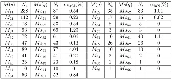
3.10 Number of terms in components of M (q) and M s(q) as well as RMS errors (eRM S) when kt = 5% and kp = 1% . . . 64

3.11 The ratio of |M1iq¨i| to |M1iq¨i|max in W1 . . . 65

3.12 Results of further simpliﬁcation for M (q)¨q . . . . 65

3.13 Actual intervals of robot states for the identiﬁcation trajectory . . . . 67

3.14 Number of terms in the simplified components and corresponding RMS errors along the identification trajectory when choosing different kt and kp . . . 68

3.15 Number of terms in components of M (q) and M s(q) as well as RMS errors along the identiﬁcation trajectory when kt= 3% and kp = 1% . 69 3.16 Number of terms in components of H(q, ˙q) and Hs(q, ˙q) as well as RMS errors along the identiﬁcation trajectory when kt = 3% and kp = 1% . . . 70

3.17 Actual intervals of robot states for the linear FSW trajectory . . . 72

3.18 Number of terms in components of M (q) and M s(q) as well as RMS errors along the linear FSW trajectory when kt= 1% and kp = 1% . . 74

3.19 Number of terms in components of H(q, ˙q) and Hs(q, ˙q) as well as RMS errors along the linear FSW trajectory when kt = 1% and kp = 1% 74 3.20 Actual intervals of robot states for the circular FSW trajectory . . . . 77

3.21 Number of terms in components of M (q) and M s(q) as well as RMS errors along the circular FSW trajectory when kt= 1% and kp = 1% . 78 3.22 Number of terms in components of H(q, ˙q) and Hs(q, ˙q) as well as RMS errors along the circular FSW trajectory when kt = 1% and kp = 1% . . . 78

(15)

LIST OF TABLES

3.24 The ratio pT(%) of the norm of all torques to the maximum one . . . 82

4.1 Robotic FSW experimental conditions . . . 92

4.2 Errors of identified models . . . 106 4.3 Value of identified parameters and their uncertainties for linear model 1106 4.4 Value of identified parameters and their uncertainties for linear model 2106 4.5 Value of identified parameters and their uncertainties for linear model 3106 4.6 Errors of identified nonlinear model . . . 112 4.7 Value of identified parameters and their uncertainties for nonlinear

model . . . 112

5.1 Parameter uncertainties, ﬁt values and RMS errors of the identiﬁed

transfer function models in three directions expressed in percentage (%) . . . 125 5.2 Identiﬁed parameters of second-order process models in three directions127

5.3 Parameter uncertainties, ﬁt values and RMS errors of the identiﬁed

second-order process models in three directions expressed in percent-age (%) . . . 127

5.4 The performance type and corresponding rise time as well as the

surface type and corresponding desired phase margin . . . 130 5.5 Actual values of gains of robot joint motion controller . . . 140 5.6 Performance comparison of three force controllers in Simulation . . . 144 B.1 Number of terms in the simpliﬁed components and corresponding

RMS errors along the linear FSW trajectory when choosing diﬀerent

kt and kp . . . 237

B.2 Number of terms in the simpliﬁed components and corresponding RMS errors along the circular FSW trajectory when choosing diﬀerent

(16)

List of Abbreviations

Abbreviations Deﬁnitions

FSW Friction Stir Welding (Soudage par frottement malaxage)

LCFC Laboratoire de Conception Fabrication Commande (in French)

Design Engineering, Manufacturing and Control Laboratory

CSC China Scholarship Council

ANR Agence Nationale de la Recherche (in French)

COROUSSO Modélisation et Commande de RObots d’USinage de pièce

composites de grandes dimensions et de SOudage FSW

IS Institut de Soudure à Goin, France (in French)

IFR International Federation of Robotics

AMF American Machine and Foundry

PUMA Programmable Universal Machine for Assembly

SCARA Selective Compliance Assembly Robot Arm

WiTP Wireless Teach Pendant

LWR Light Weight Robot

LCR Learning Control Robot

LVC Learning Vibration Control

SPT Singular Perturbation Technique

PD Proportion Diﬀerentiation

PID Proportion Integration Diﬀerentiation

DOF Degree of Freedom (degrés de liberté, ddl in French)

DGM Direct Geometric Model

IGM Inverse Geometric Model

DKM Direct Kinematic Model

IKM Inverse Kinematic Model

DDM Direct Dynamic Model

IDM Inverse Dynamic Model

SYMORO+ SYmbolic MOdelling of Robots plus

MDH Modiﬁed Denavit-Hartenberg convention

RMS Root Mean Square

XML Extensible Markup Language

LS Least Square method

RLS Recursive Least Square method

DFT Discrete Fourier Transform

(17)

LIST OF TABLES

TWI The Welding Institute (UK)

IRA Robot Institute of America

(18)

Part I

(19)

(20)

Chapter 1 General Introduction and Literature

Review

1.1 Research Background and Motivations

Friction stir welding (FSW) is a comparatively new and promising solid state welding technology developed by The Welding Institute (TWI) of UK in 1991 [1]. Compared to conventional fusion welding technologies, FSW is mainly characterized by joining material without reaching the fusion temperature, avoiding the problems caused by melting metals, such as hot cracking, solidification defects and loss of weld mechani-cal properties [2]. Almost all types of aluminum alloys can be welded through FSW process. Other advantages of FSW includes: energy efficiency, environment friend-liness, versatility, excellent weld strength and ductility, low residual stresses, no use of filler metal, relatively high welding speed and repeatability [3].

Due to the above-mentioned beneﬁts, the FSW technology has been widely ap-plied in various industrial applications. Particularly in aeronautic and astronautic industry, this technology is massively used for weight reduction. However, the fact is that the FSW process is generally carried out by some specially developed ma-chines which need a great investment. Consequently, new technologies are required to reduce the cost and improve the productivity, ﬂexibility and quality.

In recent years, robot manipulators have been increasingly used in various indus-trial applications, such as assembling, spray painting, material handling, machining and welding tasks. As for manufacturing processes, current researches focus on re-placing the dedicated machines by industrial robots due to their large working space and low cost. Although the welding performance can be greatly improved by using the industrial manipulators as tool holders, the robotization of FSW process is still an extremely challenging task at present. The limited force capability and stiﬀness of industrial robots are barriers for expansion of robotic FSW.

During the robotic FSW process, the ﬂexibility of the robot needs to be con-sidered since an extremely strong external force is exerted on the robot and a non-negligible deformation is generated. Thus, for most industrial robots applied to FSW process, a high degree of accuracy and real-time performance can not be achieved. Many studies about industrial robot control have been performed to ensure a bet-ter tracking performance. In the research work presented by Qin [4], the tracking

(21)

1.2. Literature Review on Industrial Robot Manipulators

accuracy can be enhanced by using the observer-based compensator. Due to the complicated control structure, a great deal of calculation and memory occupation will be implemented in robot controller, aﬀecting the real-time performance. Be-sides, the robust control of axial force is also required for good weld quality.

This research work is in the framework of the project COROUSSO of the pro-gram ARPEGE sponsored by the French National Agency for Research (ANR). This project aims at realizing the machining of composite materials and the FSW process with industrial robots. In this thesis, the objective is to realize the robotic FSW pro-cess with a good tracking accuracy, robust force control and real-time performance, which can be listed in detail as follows:

1) Proposition of a new simpliﬁcation method for robot dynamic model for pur-pose of improving real-time performance and related case studies;

2) Dynamic modeling and identiﬁcation of the robotic FSW process for the sake of designing the force controller of the robot;

3) Design of a robust force controller for industrial robots used in FSW process; 4) Development of a simulation system of robotic FSW process and corresponding

simulations for analyzing the performance of the force controller; 5) Vibration analysis of the axial force in the robotic FSW process.

1.2 Literature Review on Industrial Robot

Manip-ulators

According to the official definition of the Robot Institute of America (RIA), a robot is a reprogrammable multifunctional manipulator designed to move materials, parts, tools or specialized devices through variable programmed motions for the perfor-mance of a variety of tasks [5]. Furthermore, the industrial robot is also defined by the International Organization for Standardization (ISO) as an automatically con-trolled, reprogrammable, multipurpose manipulator programmable in three or more axes, which may be either mounted on fixed objects or moving objects for use in in-dustrial automation applications [6]. The typical applications for inin-dustrial robots include welding, painting, assembly, pick and place (e.g., packaging, palletizing), product inspection, and testing, etc.

1.2.1 History of Industrial Robot Manipulators

The modern history of robotic manipulation dates from the late 1940s. In order to protect technicians handling radioactive materials, the ﬁrst servoed electric-powered teleoperator was developed in 1947 [7]. Scientists initiated the research on a numer-ically controlled milling machine almost at the same time [8]. These two important technologies laid a solid foundation for the developments of industrial robots. On the basis of the report of International Federation of Robotics (IFR), a brief history of the industrial robot technology is given below [9].

(22)

Chapter 1. General Introduction and Literature Review

In 1954, George Devol applied for the first robot patent called "Programmed Article Transfer" [9]. Based on this patent, George Devol and Joe Engelberger established the first robot company known as Unimation in 1956, and developed the world’s first industrial robot Unimate in 1959. Two years later, the hydraulically powered robot Unimate was firstly installed in a General Motors (GM) automobile factory in New Jersey to extract die castings [8]. In 1962, the first cylindrical robot Versatran was introduced to the Ford factory (Canton, USA) by American Machine and Foundry (AMF). Stanford Arm invented by Victor Scheinman in 1969 was the first six-axis, electrically powered, computer-controlled robot arm, which became a standard in the design of industrial robots [10].

Industrial robots were developed for new applications as well: GM installed the first spot-welding robot at its assembly plant; Norwegian company Trallfa launched the first commercial robot for spray painting during a domestic labor shortage; Japanese company Hitachi developed the automatic bolting robot which was the first industrial robot with dynamic vision sensors for moving objects; another Japanese company Kawasaki developed the first arc welding robot Hi-T-Hand. In 1973, Ger-man company KUKA developed its own robot Famulus, the first industrial robot with six electromechanically driven axes. Cincinnati Milacron introduced the first minicomputer-controlled industrial robot T3 to market (see Figure 1.1).

Unimate Versatran Stanford Arm

Famulus T3 Hi-T-Hand

Figure 1.1: Industrial robots from 1959 to 1974 [9]

In 1974, Swedish company ASEA developed the ﬁrst fully electric, microprocessor-controlled industrial robot IRB-6, which used an Intel 8 bit microprocessor and was delivered to a mechanical engineering company in Sweden for polishing pipe bends. In Italy, the Olivetti SIGMA robot was ﬁrstly used for assembly operations with two hands. In 1978, American company Unimation/Vicarm created the PUMA (Programmable Universal Machine for Assembly) robot with support from General Motors. In the same year, the SCARA (Selective Compliance Assembly Robot Arm) robot was designed by Hiroshi Makino at University of Yamanashi in Japan. The

(23)

robot arm is slightly compliant in X-Y direction but rigid in Z direction with the help of its parallel-axis joint layout. German company Reis Robotics presented the ﬁrst six-axis robot with own control system RE15 for loading and unloading of die casting parts into trim presses. In 1979, Japanese company Nachi developed the ﬁrst motor-driven robot for spot welding.

The industrial robot industry began its rapid growth from 1980. The world’s first direct drive arm was built by Takeo Kanade at Carnegie Mellon University in 1981. The motors were installed directly into the robot joints. Due to the removal of transmission mechanisms between the motors and loads, the direct drive arm can move smoothly and freely, making it faster and much more accurate than previous robots. In the same year, Par Systems introduced its first industrial gantry robot which can provide a much larger range of motion than pedestal robots. In 1984, Adept Technology successfully marketed the first direct drive SCARA robot Adep-tOne, which is extremely robust during manufacturing processes while maintaining high precision by virtue of the simplicity of the mechanism (see Figure 1.2).

IRB-6 SIGMA PUMA

SCARA RE15 Direct Drive Arm

Nachi Gantry AdeptOne

Figure 1.2: Industrial robots from 1974 to 1984 [9]

In the early 1980s, the Delta robot (a type of parallel robot) was invented by Reymond Clavel at the Federal Institute of Technology of Lausanne (EPFL, Switzer-land) to meet the industrial need of manipulating small and light objects at a very high speed [11]. After purchasing a license for the Delta robot, the Swiss company

(24)

Demaurex sold its ﬁrst Delta robot in packaging industry market in 1992. Based on the Delta robot and image technology, ABB company developed the world’s fastest picking robot FlexPicker in 1998. The robot can pick 120 objects a minute or pick and release at a speed of 10 m/s. In 1999, Reis Robotics introduced the integrated laser beam guiding within the robot arm and launched RV6L-CO2 laser robot, which permits the robot user to operate laser device at high dynamics.

The robot control system also achieved a great development. In 2004, Japanese company Motoman introduced the improved robot control system NX100, which is able to control four robots synchronously (up to 38 axis). Two years later, Italian robot company Comau launched the ﬁrst Wireless Teach Pendant (WiTP), enabling robot data communication to be implemented without a cable connection.

Delta FlexPicker RV6L-CO2

WiTP KUKA LWR FANUC LVC

Figure 1.3: Industrial robots from 1985 to present [9]

In 2006, KUKA company presented the first Light Weight Robot (LWR), which weighs only 16 kg but has a payload capacity of 7 kg. The robot is portable and energy-efficient and can carry out a great variety of tasks. The first Learning Control Robot (LCR) was launched by FANUC in 2010. The robot can learn its vibration characteristics through Learning Vibration Control (LVC), and suppress the vibra-tion to reduce the cycle time of robot movibra-tion (see Figure 1.3).

1.2.2 Current Developments of Industrial Robots

According to the IFR report of World Robotics in 2014, the total worldwide stock of operational industrial robots reached at least 1332000 units at the end of 2013. About 52% of the industrial robots are in Asia, 29% in Europe, and 17% in North America. It is estimated that global robot installations will increase to 1946000 by the end of 2017 [12].

From 2003 to 2013, the worldwide annual installations of industrial robots are summarized in Figure 1.4. Due to the improved global economic situation, the

(25)

robot sales in 2013 increased by 12 % to 178132 units, which is the highest number of industrial robots ever sold. In 2013, most of the robot sales (about 70%) were in ﬁve countries: China, Japan, the United States, South Korea and Germany. It should be noted that China became the world’s biggest and fastest growing robot market with a share of 20% of the total supply. Industrial robot sales to almost all industries gained strong growth, including automotive, electronics, metal, rubber and plastics industries as well as food industry.

Figure 1.4: Worldwide annual installations of industrial robots [12]

The worldwide market value for industrial robots was up to 9.5 billion US dollars in 2013. Including the cost of software, peripherals and systems engineering, the turnover for robot systems was estimated to be 29 billion US dollars. Most of the industrial robots around the world are designed and made by several famous and inﬂuential industrial robot companies, such as ABB Robotics, FANUC Robotics, KUKA Robotics, Yaskawa Electric and Kawasaki Robotics, etc.

ABB IRB 7600 KUKA KR1000 TITAN F FANUC M-2000iA/1200 Yaskawa MH400 II

Figure 1.5: Industrial robots launched by four diﬀerent companies

Figure 1.5 shows the industrial robots with high payloads which can carry out a wide range of manufacturing processes. The information about the various industrial robots launched by the four companies can be found in [13, 14, 15, 16].

(26)

1.3 Literature Review on Modeling of Flexible Joint

Robot Manipulators

In most cases, the heavy industrial robots can be considered as rigid since the force exerted on the robot during the manufacturing process is not very large. Conse-quently, the deformation of the robot due to its ﬂexibility can be neglected. How-ever, the ﬂexibility must be taken into account when the robot carries out some applications which need large working force.

As for industrial manipulators, the flexibility can be supposed as concentrated at the robot joints or distributed along the robot links in different ways from a modeling point of view [7]. According to the research work of Dumas [17], the main sources of flexibilities for the serial industrial robots are the flexibilities located at the robot joints (including motors and transmissions). Based on this study, the links of industrial robots used in this research should be considered as rigid. The modeling and control problems of industrial manipulators with flexible joints will be mainly concerned hereafter.

In fact, the joint flexibility of the current industrial robots comes from the mo-tion transmission/reducmo-tion elements, such as belts, cables, long shafts, harmonic drives and cycloidal gears. These components are utilized to allow relocation of the actuators next to the robot base, improving dynamic efficiency. However, these components are intrinsically flexible when subject to the working force during the robot operation [7].

The early study of the problems caused by flexible transmissions in robot ma-nipulators can be found in [18, 19], with first experimental findings on the GE P-50 arm. In 1987, Spong proposed a simplified flexible joint model and considered the joint flexibility as a linear torsional spring with a stiffness constant [20, 21]. Based on the dynamic model of Spong, Khorasani established a single-link rigid-flexible coupled model, in which the influence of the damping term and harmonic gear is taken into account [22].

The simplified flexible joint model proposed by Spong is valid only in the case of large gear ratios because the cross inertial effects could be ignored in that situation. Thus, Tomei proposed a complete flexible joint model by including the couplings between the links and the motors [23].

The precision of a robot model can be greatly influenced by the nonlinear charac-teristics of the gear transmission, which mainly contain the friction and the nonlinear stiffness. It should be noted that the nonlinear stiffness can be also included in the flexible joint model by replacing the linear stiffness formulation with a nonlinear function describing a nonlinear spring. More nonlinearities can be added to the flex-ible joint dynamic model, such as backlash, hysteresis and nonlinear damping [24]. A relatively precise flexible joint robot dynamic model was proposed by Bridges and proved to be stable. In this model, the friction, nonlinear flexibility, and kinematic errors are taken into consideration [25].

Moberg proposed an extended ﬂexible joint model where the elasticity is de-scribed by a number of localized multi-dimensional spring-damper pairs [24]. This spring-damper pair is able to have up to six degrees of freedom and includes both translational and rotational deﬂection.

(27)

1.4. Literature Review on Control of Flexible Joint Robots

1.4 Literature Review on Control of Flexible Joint

Robots

Generally, the types of commonly used control laws contain: linear or nonlinear, static or dynamic, feedback dominant or feedforward dominant, discrete-time or continuous-time, robust or adaptive, diagonal or full matrix, etc.

Early researchers mainly focused on studying the impact of motor dynamics on control performance in the field of robot control. However, in 1985 Sweet and Good pointed out that joint flexibility should be taken into account in both modeling and control if high tracking performance is required [18]. In 1987, Spong proposed a simplified flexible joint model [20]. Since then a lot of theoretical and experimental research had been performed on controlling flexible joint robots: singular pertur-bation and integral manifold, feedback linearization, cascaded system and integral backstepping, PD control, adaptive control, robust control, neural networks, fuzzy control and some other control methods.

1.4.1 Singular Perturbation and Integral Manifold

Flexible joint robot can be considered as a weak elasticity system if its joint stiﬀness is large enough. This feature makes it possible that we transform the ﬂexible joint model into a two-time-scale (FTS: Fast Time Scale and STS: Slow Time Scale)

system by using singular perturbation technique. In system dynamics, singular

perturbation technique (SPT) is widely applied to the system which can be divided into a fast subsystem and a slow subsystem. With the advantage of model reduction, this technique can decompose a high-order system into two lower-order systems. The core idea is based on adding a simple correction term to the control law for rigid body robots to damp out the elastic oscillation at the joints. However, the approach only can be used in robot systems with weak joint ﬂexibility, where the ﬂexible dynamics is much faster than the rigid-body dynamics.

Singular perturbation model for the same system is not unique. Spong presented a control design modeling the joint elastic forces as the fast variables and the link variables as the slow variables [21]. Ge proposed a new adaptive controller based on SPT and using only position and velocity feedback by modeling the motor tracking error as the fast variables and the link variables as the slow variables [26]. As a consequence, the slow time-scale dynamics and the resulting control laws are also diﬀerent from those given by Spong.

However, the dynamical systems obtained by decomposition based on SPT are extremely complex to control, and a need for order reduction and simpliﬁcation is inevitable. In order to solve this problem, some researchers introduced the concept of integral manifold. The integral manifold is a tool for reduced-order modeling because if the system trajectories are on the manifold, then a 2nth-order slow model is an exact representation of the 4nth_{-order system [27]. This fact will be used to construct}

corrected reduced-order models. By using this idea to represent the dynamics of the slow subsystem, Spong derived a reduced-order model of the manipulator which incorporates the eﬀects of the joint ﬂexibility on the system [21].

(28)

After obtaining the reduced-order systems, various control methods can be di-rectly applied, such as robust control [28], fuzzy control [29], etc. Ghorbel and Spong ﬁrst proposed an adaptive composite control strategy for ﬂexible joint robot manip-ulators, which is also called fast/slow control strategy consisting of a slow adaptive controller designed for a rigid robot together with a fast control to damp the elastic oscillations of the joints [30], and gave its local stability analysis [31]. Compared with the method of feedback linearization, this approach, which is based on integral manifold, can overcome the need for feedback of link acceleration and jerk, but lacks of robustness to parametric uncertainty. Then they extended the integral manifold approach from the known parameter case to the adaptive one [32], and clear draw-backs of this adaptive integral manifold is its complexity of expression derivation and computational burden.

Some researchers also studied the robustness issue of control method based on singular perturbation and integral manifold. Taking the unmodeld dynamics and parameter vibrations into account, Khrasani corrected the perturbed equations, and obtained a reduced-order flexible model without parametric uncertainty so that the feedback linearization and robust adaptive control strategies could be applied to control flexible joint robots [33]. Al-Ashoor developed a robust adaptive controller, which was designed to compensate for the effects of unmodeled dynamics and the errors arising from parameter vibrations and neglecting higher order effects of joint flexibility [34].

Although SPT has the advantage of order reduction and can use adaptive control algorithm to get more accurate parameter, it is difficult to find an adaptive control law for a nonlinear system and the computational burden is high. Furthermore, this approach is limited by joint stiffness. In order to solve this problem, Liu designed a joint flexibility compensator which can greatly increase the equivalent joint stiffness so that the approach can be extended to the robot system with normal joint flexibility [35]. But the universality cannot be proved because he only realized this controller in a single joint.

1.4.2 Feedback Linearization

Feedback linearization is regarded to be a better method to control a nonlinear system. The core idea of this method is to transform the original nonlinear system to an equivalent linear system by using suitable nonlinear state transformation and correct control law, in order that it is convenient to apply the control methods of the linear system to this equivalent linear system. From a theoretical standpoint, this method is considerably attractive because it is easy to prove the stability of the system, that is to say, the original nonlinear system is stable if the stability of its equivalent linear system is proved. This method is widely used in the control of rigid robots, such as computed torque control and inverse dynamics control. This is because the models of rigid robot can always be feedback-linearized. However, some dynamic models of ﬂexible joint robots cannot meet requirements of feedback linearization.

Spong proposed a simplified flexible joint model where the joint flexibility is con-sidered as a linear torsional spring and the kinetic energy of the rotor is due mainly to

(29)

its own rotation. He also pointed out that this simplified model system can be glob-ally linearized by nonlinear coordinate transformation and static state feedback [20]. Then Grimm performed a robustness analysis of feedback-linearized or nonlinear-decoupled control loops for simplified flexible joint model [36]. Sira-Ramirez and Spong proposed an outer-loop control based on the sliding mode theory of variable structure systems for robust tracking [37]. Ge designed a robust adaptive neural net-work controller for the flexible joint robots using feedback linearization techniques, and it could better handle dynamical model changes and parameter uncertainties than the conventional feedback linearization controller [38]. Ider proposed a trajec-tory tracking control law for flexible joint robots based on solving the acceleration level inverse dynamics equations which are singular, and the implicit numerical in-tegration method was used to avoid further differentiation of the motion and task equations [39].

As for complete dynamic model of ﬂexible joint robots, it cannot be linearized only by static state feedback. However, De Luca proved that the complete dynamic model can always be fully transformed into a linear, controllable and input-output decoupled system by nonlinear dynamic state feedback if the system is invertible with no zero dynamics [40]. He introduced a general inversion algorithm for the synthesis of a dynamic state feedback law that gives input-output decoupling and full state linearization [41].

The feedback linearization control law requires high-order diﬀerential terms, such as acceleration and jerk. It means some state must be estimated from available measurements, for example, the jerk. So we have to construct suitable observers to perform states estimation.

In conclusion, tracking performance of feedback linearization control depends heavily on model accuracy of the system. Meanwhile, a linear or a nonlinear ob-server needs to be constructed because all states for feedback computation must be obtained, making the system more complex. So one approach is to combine feedback linearization with adaptive control or neural network control to reduce the require-ment of model accuracy. Another approach is to use the controller with no need for all states feedback.

1.4.3 Cascaded System and Integral Backstepping

Cascaded system method firstly assumes that dynamics related to rigid manipula-tors can be controlled directly, then decides the actuator control law by taking the flexibility of joints into consideration. In this method, the dynamic model of flexible joint robots is expressed in the form of two cascaded loops: the manipulator loop and the actuator loop regarding the flexibility of the joint. A desired force which is introduced as a synthesized input signal for the manipulator loop, is generated due to the flexibility between the motor and the link. And it must be realized by the output of the actuator loop through designing a suitable controller. Compared with singular perturbation technique, this method is not subject to restrictions on the magnitude of the joint flexibility.

Cascaded system method depend on a better system model, therefore it usually requires a combination of the adaptive control law. Yuan developed a composite

(30)

adaptive controller for ﬂexible joint robots without any restrictions on joint stiﬀness by using this method [42]. The paper [43] proposed adaptive task-space controllers to solve motion control and compliance control problems.

Integral backstepping control technique has recently been developed for the cas-caded systems. This systematic method is realized by designing a Lyapunov function for the system whose input side has a series of integrators, and it becomes an im-portant theoretical design method because the method can provide the proof of Lyapunov stability.

Three improvements obtained from integral backstepping technology are (1) the ability to construct globally stable controllers that compensate for parametric un-certainty, (2) the elimination of restrictions on the magnitude of the joint ﬂexibility, and (3) the elimination of the requirement of link acceleration and link jerk mea-surements. All of the above improvements, however, are not fully exploited at once. For instance, Chen and Fu developed a controller which can eliminate restrictions on the size of joint ﬂexibility, but can only compensate for parametric uncertainty to the extent of proving local stability. In addition, link acceleration measurements are needed, and this is not practical for most industrial robots [44]. Beneallegue and Sirdi used a passivity approach to design a globally asymptotically stable adaptive controller, but it needs both link acceleration and jerk measurements [45].

The above methods have dealt with parametric uncertainty by using an adap-tive approach with asymptotic position tracking as the goal but have been plagued by the requirement of either link acceleration or jerk measurements. Dawson used a backstepping approach to design a robust controller that compensates for para-metric uncertainty and unknown bounded disturbances while achieving a globally uniformly ultimately bounded position tracking error [46]. Nicosia and Tomei made a further step to design an adaptive controller that can simultaneously satisfy the above three improvements, but it is special for a single-link ﬂexible joint robot still leaving a control problem for general n-link ﬂexible joint robots [47]. Lozano and Brogliato solved the problem and designed an adaptive control scheme achieving globally asymptotic position tracking while satisfying the three improvements [48]. In their method, inverse inertia matrix is required to eliminate the measurements of the link acceleration, increasing the computational time and complexity.

Kwan and Lewis proposed a robust backstepping controller using neural networks [48]. Compared with adaptive backstepping control, linearity in unknown param-eters is not needed. A major problem with backstepping is corrected in that no tedious computation of ’regression matrices’ is needed. However, most neural net-works need a long training time, and it is not practical for robot real-time control. Macnab and D’Eleuterio developed a neuroadaptive control scheme using a rela-tively small neural network, which is more practical to implement owing to reduced training times and reduced on-line computational burden [49].

Although integral backstepping technology is not subject to restrictions on the size of joint ﬂexibility, it still needs more complete research. It usually contains an adaptive control law because it is sensitive to model parameters. Another problem with backstepping is that the constructed Lyapunov equation is limited and it does not have a parameter to adjust the system performance directly, while its only

(31)

advantage is the guarantee of system stability. More materials can be seen in a survey of backstepping approach for ﬂexible joint robots [50].

1.4.4 PD Control

Traditional PD (or PID) controllers are widely used in practical engineering for simplicity, strong robustness and high control precision. In engineering, a modified PD controller with a joint flexibility compensation can be used in the control of flexible joint robots.

A simple PD controller suffices to stabilize any kind of rigid robot about a ref-erence position if gravitational forces are compensated. Although rigid robots are exactly linearizable by static-state feedback, the stability of the PD controller does not rely on this property, but it is rather related to the intrinsic passivity properties. Tomei proposed a simple PD controller and demonstrated its global asymptotic sta-bility [23]. Albu-Shaffer and Hirzinger developed a joint state feedback PD controller with gravity and nonlinear friction compensation, which can be gradually extended to take account of the full robot dynamics. The global asymptotic stability was proven based on Lyapunov’s first method, and effectiveness of the controller was validated through experiments on a 7 d.o.f. lightweight manipulator [51].

Although PD control is simple and useful, the joint ﬂexibility must be taken into account in modeling of the robot in order to improve control accuracy.

1.4.5 Other Control Methods

In addition to the above-mentioned control methods, adaptive control, robust con-trol, neural networks, fuzzy concon-trol, sliding mode control [37], etc., are also applied to the control of ﬂexible joint robots.

Adaptive control and robust control are two basic control strategies for solving problems of robot uncertainties, such as uncertainties of model parameters, unknown or varying loads, flexibility of joint, time-varying friction coefficient, etc. When parameters of the controlled system change, adaptive control [26, 30, 32, 33, 34, 38, 42, 43, 45, 47, 49, 52, 53, 54] can achieve certain performance by identification, learning and adjustment of the control law. But it cannot guarantee the stability of the system when strict real-time requirement is proposed and implementation is complex, especially when non-parametric uncertainty exists. However, robust control [28, 33, 34, 37, 38, 46, 48, 55, 56, 57] can guarantee the stability of the system and maintain a better performance when the uncertainties are in a certain range.

Since the accurate model of the ﬂexible joint robot can not be obtained, neural network control [38, 48, 49, 58] is proposed to solve this problem through learning the unknown model information and training the neural network to approximate the system dynamics.

Fuzzy control [29] dose not require a precise system model in controller design, and generally it needs the experience from user or expert, information and opera-tional data, etc. It is convenient to obtain the control strategy for nonlinear and uncertain objects, and has a good real-time performance due to its simple algorithm.

(32)

For typical robotic tasks (e.g. machining and FSW process) that require inter-action with the environment, contact forces must properly be handled by the robot controller. In such cases, a pure motion controller usually gives poor performance and can even cause instability. Chiaverini et al. proposed a stable force/position control scheme for the robots in contact with an elastically compliant surface, and it was tested on the industrial robot COMAU SMART 6.10R [59]. De Luca also de-signed a robust hybrid control scheme for force and velocity control of manipulators in dynamic contact with the environment [60].

1.5 Dissertation Outline

This thesis report is composed of the following six chapters:

Chapter 1 oﬀers the general introduction of the thesis, including the background of the thesis, the research problems and objectives, a literature review based on a deep and extensive literature study and the outline of the dissertation.

Chapter 2 presents the modeling of the flexible joint robot manipulators. Sev-eral essential models of a 6-DOF flexible joint robot manipulator including direct geometric model (DGM), inverse geometric model (IGM), direct kinematic model (DKM), inverse kinematic model (IKM), direct dynamic model (DDM) and inverse dynamic model (IDM) are established based on the fundamental knowledge concern-ing the robot modelconcern-ing, such as the spatial descriptions, the homogeneous transfor-mations, the X-Y-Z fixed angles and the modified Denavit-Hartenberg convention, etc. Besides, the joint flexibility model, the friction model and the torque of gravity compensator at the second axis are studied as well.

Chapter 3 proposes a novel approach for the simplification of industrial robot dynamic model based on interval method. Firstly, the basic definitions and oper-ations of interval analysis as well as the inclusion function and overestimation are introduced. Then, the symbolic dynamic model of an industrial manipulator KUKA KR500-2MT is generated. Next, a generalized simplification algorithm is proposed and a simple example is provided to explain and describe the simplification method. Meanwhile, the results of the simplified model for the whole workspace and corre-sponding error analysis as well as the further simplification are also given. Case studies have been carried out on three different test trajectories including the iden-tification trajectory, the linear FSW trajectory and the circular FSW trajectory, in order to demonstrate the performance of the simplification method. Moreover, the torques in the robot dynamic equation has been analyzed in the case of a linear FSW process as well. Finally, some usages of the simplification method are provided.

Chapter 4 presents the dynamic modeling and identification of the robotic FSW process. First of all, a brief description of the FSW process is given, including its main stages and process forces as well as two static nonlinear power models of the process forces. Then, the experimental setup for the model identification is de-scribed. In the meantime, three methods which can calculate the plunge depth and its derivative are proposed, followed by the data filtering for the measurements and calculations. Next, the linear and nonlinear dynamic modeling and identification of the axial force are implemented by using least squares method. Finally,

(33)

system-1.5. Dissertation Outline

atic studies on the errors of identiﬁed models have been carried out to analyze the performance of the model identiﬁcation.

Chapter 5 describes the design of robust force controllers for industrial robot manipulators and the development of a simulation system of robotic FSW process. Firstly, a literature review on force control methods of the robot is presented, fol-lowed by selecting the force control strategy and the modeling of the robotic FSW process. Then, the parameter identification of rigid robot displacement model is implemented by using two different algorithms. Based on the modeling of robotic FSW process which simultaneously considers the complete kinematics, the rigid robot displacement model, the joint flexibility and the dynamic axial force process model, the robust force controllers have been designed by using the frequency re-sponse approach. Next, the simulator of robotic FSW process is established and simulation studies have been carried out to test the performance of force controllers. Finally, the axial force vibration in robotic FSW process is analyzed and a distur-bance model of zero force vertical position which can lead to the oscillation of axial force is proposed and used in simulations.

Chapter 6 concludes the thesis with main contributions of the research and perspectives for the future work.

Chapter 1 Background; Motivations; Literature review on industrial robots, modeling and control of

flexible joint industrial robots; Dissertation outline

Chapter 2 Modeling of flexible joint

robot manipulators

Chapter 3

Simplificaition of robot dynamic model using interval method

Chapter 4

Dynamic modeling and identifi -cation of robotic FSW process

Chapter 5

Design of robust force controller in robotic FSW process

Chapter 6 General conclusions (main contributions); Discussions & Perspectives

(34)

Chapter 2 Modeling of Flexible Joint Robot

Manipulators

2.1 Introduction

The work presented in this chapter concerns the modeling of flexible joint robot manipulators. Based on a lot of research work on robot modeling described in the books of Craig [62], Spong [8], and Siciliano [5], the fundamental studies are carried out in order to obtain the different models which we need to use in the model simplification, simulation of robot motion and controller design. Thus, the work in this chapter is an important foundation for the following research.

Section 2.2 gives a brief introduction to the spatial description and coordinate transformation in robotics. Then, section 2.3 focuses on the problem of robot kine-matics. The direct and inverse geometric models, the direct and inverse kinematic models are also established. In Section 2.4, the dynamic model, the ﬂexibility model and the friction model of the robot are studied. The software SY M ORO+ for generating symbolic robot models is introduced as well.

2.2 Spatial Descriptions and Coordinate

Transfor-mations

2.2.1 Descriptions of Positions, Orientations and Frames

Generally, the concepts of position vectors, planes and coordinate frames will be used to describe the relationship between some objects, including parts, tools, and the manipulator itself.

In the selected Cartesian coordinate frame {A}, arbitrary point P in space can be represented as a 3× 1 position vector A_{P :}

A P =    px py pz    (2.1)

Modélisation d'un robot manipulateur en vue de la commande robuste en force utilisé en soudage FSW

HAL Id: tel-01305951

https://pastel.archives-ouvertes.fr/tel-01305951

Modélisation d’un robot manipulateur en vue de la

commande robuste en force utilisé en soudage FSW

Ke Wang

To cite this version:

École doctorale n° 432 : Science des Métiers de l’Ingénieur

Ke WANG

Robot manipulator modeling for robust force control

used in Friction Stir Welding (FSW)

~~~

Modélisation d’un robot manipulateur en vue de

la commande robuste en force utilisé en soudage FSW

Doctorat ParisTech

T H È S E

l’École Nationale Supérieure d'Arts et Métiers

Spécialité “ Automatique ”

T

H

È

S

E

Contents

I

English Version

15

II

Résumé Étendu en Français

159

Acknowledgements

List of Figures

List of Tables

List of Abbreviations

Part I

Chapter 1

General Introduction and Literature

Review

1.1

Research Background and Motivations

1.2

Literature Review on Industrial Robot

Manip-ulators

1.2.1

History of Industrial Robot Manipulators

1.2.2

Current Developments of Industrial Robots

1.3

Literature Review on Modeling of Flexible Joint

Robot Manipulators

1.4

Literature Review on Control of Flexible Joint

Robots

1.4.1

Singular Perturbation and Integral Manifold

1.4.2

Feedback Linearization

1.4.3

Cascaded System and Integral Backstepping

1.4.4

PD Control

1.4.5

Other Control Methods

1.5

Dissertation Outline

Chapter 2

Modeling of Flexible Joint Robot

Manipulators

2.1

Introduction

2.2

Spatial Descriptions and Coordinate

Transfor-mations

2.2.1

Descriptions of Positions, Orientations and Frames