Compliant riblets: problem formulation and effective macrostructural properties

Any correspondence concerning this service should be sent

to the repository administrator:

tech-oatao@listes-diff.inp-toulouse.fr

This is an author’s version published in:

http://oatao.univ-toulouse.fr/24303

To cite this version:

Zampogna, Giuseppe Antonio and Naqvi, Sahrish Batool and

Magnaudet, Jacques and Bottaro, Alessandro Compliant

riblets: problem formulation and effective macrostructural

properties. (2019) Journal of Fluids and Structures, 91

(November). 1-14. ISSN 0889-9746

Official URL:

Compliant riblets: Problem formulation and effective

macrostructural properties

Giuseppe A. Zampogna

a,1

_{, Sahrish B. Naqvi}

b

_{, Jacques Magnaudet}

a

_,

Alessandro Bottaro

b,∗

a_{Institut de Mécanique des Fluides de Toulouse (IMFT), Université de Toulouse, CNRS, INPT, UPS, Toulouse, France} b_{Dipartimento di Ingegneria Civile, Chimica e Ambientale, Università di Genova, Via Montallegro 1, Genova, 16145, Italy}

a b s t r a c t

Small-scale, deformable riblets, embedded within the viscous sublayer of a turbulent boundary layer and capable to adapt to the overlying motion, are studied. The wall micro-grooves are made of a linearly elastic material and can undergo small deforma-tions; their collective behavior is assumed to occur over a large, elastic wavelength. The presence of two length scales allows for the use of a multiscale homogenization approach yielding microscopic problems for convolution kernels and parameters, which must then be employed in macroscopic boundary conditions to be enforced at a virtual wall through the riblets. The results found suggest that, in analogy to the case of rigid riblets, compliant, blade-like wall corrugations are more effective than triangular riblets in reducing skin friction drag, provided the spanwise periodicity of the indentations is sufficiently small for the creeping flow approximation to be tenable.

1. Introduction

Riblets are elongated micro-grooves at the wall, aligned with the direction of the main flow. They represent a mature passive control technology aimed at reducing skin friction drag in turbulent flow, which has been successfully tested both in the laboratory and in aeronautical/marine applications.

Apart from a general agreement that riblets can reduce the frictional drag in a turbulent boundary layer by as much as 7%

−

8% (Walsh and Lindemann,1984), the manner by which a turbulent near-wall flow reacts to the presence of riblets was not fully understood in early research. A possible physical mechanism for drag reduction was reported by Chu and Karniadakis (1993) as being related to the limited interaction between near-wall quasi-streamwise vortices and the surface with micro-grooves. This seemed to balance the fact that the wetted area in the case of a ribbed wall increased when compared to the smooth-wall case. Complementary experimental and numerical work on triangular riblets in the laminar regime was conducted by Djenidi et al.(1994). Since these authors found that skin friction drag was not increased with respect to the flat-wall case, under the same working conditions, the importance of the flow viscous response was highlighted. Subsequent research focussed on the viscous near-wall flow, to extract salient features of microstructured surfaces. Today, the mechanism by which riblets operate is believed to be related to the creation of an offset between the virtual origin of the longitudinal mean flow and that of the transverse turbulent eddies. Provided

∗ _{Corresponding author.}

E-mail address: alessandro.bottaro@unige.it(A. Bottaro).

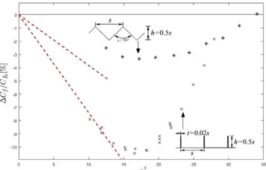
Fig. 1. Experimental drag reduction data (symbols) for triangular and blade riblets. The straight dashed lines correspond to the linear regime for

the two wall corrugations considered, as by Eq.(1).

Source: Adapted fromBechert et al.(1997).

that the riblets are embedded in the viscous sublayer, their effect can be modeled by the Stokes equation to yield two distinct protrusion heights, or Navier’s slip lengths, longitudinal,

λ

1, and transverse,

λ

2, which are the distances from the

rim of the riblets to the position where, respectively, streamwise and cross-stream flows originate. These concepts have been introduced byBechert and Bartenwerfer(1989) andLuchini et al.(1991), and tested experimentally byBechert et al. (1997), among others. The results show that riblets remain in the linear (Stokes) regime as long as their dimensionless spanwise periodicity, s+

, measured in viscous wall units, remains below a value close to 10 (cf.Fig. 1). The optimal riblet spacing is about 15 for a variety of riblet shapes, and skin friction drag can be reduced by at most 10% in the case of thin, blade-like riblets (Bechert et al.,1997). Above s+

≈

15, drag starts increasing again and, for s+

≳ 30, the skin friction coefficient exceeds the value of the corresponding smooth wall because of the appearance of a Kelvin–Helmholtz-like instability of the mean flow which increases the spanwise coherence of the turbulent structures, therefore disintegrating the longitudinal streaks, via the creation of spanwise rollers (García-Mayoral and Jiménez,2011).

For drag to decrease, for any kind of wall indentation fully immersed in the viscous sublayer, the origin of the secondary flow must be farther away from the base of the indentation than the origin of the mean streamwise motion or, in other words,∆

λ = λ

1

−

λ

2must be positive. When this occurs, crossflow is impeded (more than the longitudinal flow) and

high velocity bursts from the surface are mitigated, resulting in smaller drag. The amount by which drag reduction is achieved is given to leading order in∆

λ

by

∆Cf Cf0

= −

∆

λ

+ (2 Cf0) −1/2

₊

₍₂

κ

₎−1

,

(1)

as first shown byLuchini(1996). In Eq.(1), Cf is the skin friction coefficient, Cf0 its value for the case of a smooth surface

under the same outer flow conditions, and

κ =

4

.

48 is von Kármán’s constant (Luchini,2018). Despite the fact that the equation above holds only in the initial part of the drag curve, the agreement of this theoretical estimate with experiments is satisfactory and strongly endorses the idea of maximizing∆

λ

when drag reduction is sought for.Fig. 1demonstrates the advantage of using blade riblets (of thickness t equal to 0

.

02 s in the case of the figure) as compared, for example, to triangular riblets with a top opening angle of 90o_{. It is also interesting to observe that the theoretical results embodied}

by Eq.(1)(and shown with dashed lines in the figure) are in excellent agreement with the experimental data for blade riblets almost until the point of maximal drag reduction (close to s+

₌

15), whereas for the triangular wall corrugations the range of validity of the theoretical result is smaller and extends to s+

≈

5.

Another aspect of the near-wall indentations which deserves attention is the possibility for the solid material at the fluid–solid interface to deform under the action of the fluid. Research on elastic and viscoelastic interfaces has enjoyed waves of renewed attention in the past fifty years, coinciding with the growing or diminishing interest of funding agencies. The initial stimulus to the idea of using compliant surfaces for drag reduction came fromKramer(1957,1961), who ascribed the extraordinary swimming ability of dolphins to the pliability of their skin. Kramer’s argument was that

3

shear layer fluctuations were damped near the dolphin’s compliant dermis, thus leading to extended regions of laminar flow on the body. This, is turn, was assumed to be the cause of drag reduction. Much research ensued, particularly on the onset of transition to turbulence for the flow over compliant walls, culminating with the modeling efforts of Peter W. Carpenter and collaborators (Carpenter and Garrad,1985,1986;Dixon et al.,1994;Carpenter et al.,2000). On the experimental side,Gad-el-Hak et al.(1984) performed several experiments in a water channel with a flat plate coated with a compliant material, under laminar, transitional and turbulent conditions, highlighting the presence of hydroelastic instabilities capable to lead to early transition and rise in drag. Turbulent drag increase was typically associated to the appearance of a large-amplitude deformation of the compliant surface, resulting from a static-divergence instability. Conversely, when the surface deformation of the wall was maintained significantly within the viscous sublayer (for the wall to remain hydrodynamically smooth), some success in reducing skin friction drag by the use of compliant viscoelastic panels was reported (Lee et al.,1993;Choi et al.,1997). Drag reduction was accompanied by reduction of the turbulent intensity across the boundary layer.

When the wall is rough, little attention has been paid to the dynamic role of deformable roughness elements, aside, possibly, for the case of terrestrial and aquatic canopies (De Langre,2008;Nepf,2012). In these configurations, however, the vegetation extends beyond the viscous sublayer and its effect differs from that found in canonical rough turbulent boundary layers. Significant studies on the interaction between near-wall turbulence and flexible micro-protrusions are very recent and the picture which emerges is not yet complete. The experimental work byToloui et al.(2019) considered a regular pattern of cylindrical micro-elements, orthogonal to the wall of a water channel and embedded within the boundary layer. They used holographic particle tracking velocimetry to find that the Reynolds stress over the flexible roughness elements was smaller than that over their rigid counterpart; this reduction was accompanied by a decrease of coherence of the roughness-induced flow structures. In the numerical study by Sundin and Bagheri(2019) a similar set-up was considered and a systematic analysis was conducted by varying the relative magnitude of the natural frequency of the cylindrical fibers to the characteristic frequency of cyclic events of near-wall coherent structures; this could be achieved simply by changing the density of the wall protuberances, compared to that of the fluid, for a fixed modulus of elasticity of the solid. The fibrous bed was found to rapidly react to the turbulence when the fibers had a density comparable to that of the fluid (i.e. when the fibers’ natural frequency was much larger than the frequency of turbulent events), resulting in destruction of the streaks and significant drag increase. Conversely, when the fibers had a density much larger than the fluid density, the fibrous bed reacted slowly to the flow and the turbulent coherent structures were not very different from the smooth-wall case.

The idea of combining the presence of regular micro-grooves with the fact of rendering them elastic stems from the realization that frictional drag in turbulent flows decreases when the spanwise motion of the streaks is hampered (Choi, 1989; Lee and Choi,2008). This effect is possibly achieved by combining the properties of a compliant material with the design of appropriate micro-indentations. It is thus aimed for compliance to impair the lateral movement of the streaks, reducing violent ejections and bursts, with a positive effect on skin friction resistance. A further consideration applies: the optimal geometrical characteristics of riblets depend on the outer flow conditions, and what is optimal for one condition (say, level flight of an aircraft at cruise speed) may not be optimal any more under different conditions. Suitably designed microstructures capable to deform elastically and adapt to the outer flow conditions might provide an answer to this practical shortcoming. Recently, a patent has been submitted describing the manufacturing of elastomeric riblets (Rawlings and Burg,2016), with the claim that their optimized structural design provides the capability for riblets to be ‘‘thinner, lower weight and more aerodynamically efficient’’.

The arguments given above justify the interest in examining the interaction between elastic, streamwise-elongated wall corrugations and the overlying fluid. We call these indentations compliant riblets. The goal of this study is to develop the mathematical tools to describe compliant riblets, to set the framework in order to optimize their geometrical and structural properties, for drag reduction purposes. The present contribution is thus dedicated to the study of the interface problems, in both the fluid and the solid domains, for prototypical triangular and blade riblets such as those shown in Fig. 1, made of a linearly elastic material. The main outcome of the work will be the macroscopic equations ruling the fluid–solid interactions, plus the effective coefficients (or convolution kernels, by virtue of the time dependent nature of the fluid–solid coupling) required to close the macroscopic problem. Clearly this work is but the first step of a more comprehensive examination on the effect and design of compliant riblets; the considerations made possible by the analysis reported herein represent a promising path for future investigations.

2. Model development

An incompressible Newtonian fluid of density

ρ

f and viscosity

µ

is assumed to flow over a micro-patterned surface

made of a linearly elastic material of density

ρ

s, Poisson’s ratio

ν

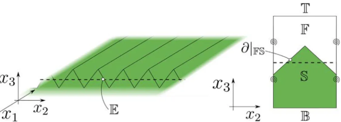
P and Young’s modulus E. A sketch of the surface being

considered is represented inFig. 2. The objective of this model is to simulate the fluid flow and solid structure deformation without the need of large computational efforts to describe the details of the solid surface and solve the small-scale fluid–solid interactions. The procedure shown in the present section gives rise to equivalent boundary conditions for the macroscopic fields associated with the solid displacement and fluid flow. These boundary conditions must be imposed on an equivalent smooth surface (denoted with E inFig. 2) which is located at a certain (small) distance from the tip of the

Fig. 2. Sketch of a deformable, regularly micro-structured surface. Right frame: a periodic unit cell is identified to apply the homogenization technique.

small-scale protrusions. To proceed with the development of these conditions, we introduce the fluid domain, denoted by F inFig. 2, in which the incompressible Navier–Stokes equations are valid and write in dimensional form

ρ

f

(

∂ ˆ

ui

∂ˆ

t

+ ˆ

uj

∂ ˆ

ui

∂ ˆ

xj

)

=

∂ ˆ

Σij

∂ ˆ

xj

,

(2)

∂ ˆ

ui

∂ ˆ

xi

=

0

,

(3)

where_Σ

ˆ

_{ijis the canonical fluid stress tensor of a Newtonian fluid}

ˆ

Σij

= − ˆ

p

δ

ij

+

2

µˆε

ij(u)

ˆ

,

(4)

and

ε

ˆ

_ij(u) is the strain-rate tensor, formally defined as

ˆ

ˆ

ε

ij(u)

ˆ

=

1 2

(

∂ ˆ

ui

∂ ˆ

xj

+

∂ ˆ

uj

∂ ˆ

xi

)

.

(5)

In the domain S occupied by the linearly elastic solid, the governing equations read

ρ

s

∂

2

_v

_ˆ

i

∂ˆ

t2

=

∂ ˆσ

ij

∂ ˆ

xj

,

(6)

where

v

ˆ

i denote the components of the displacement vector,v, and

ˆ

σ

ˆ

ijis the generic component of the stress tensor.

Under the assumption that the structure is elastic, the stress and strain tensors are linearly related through the relation

ˆ

σ

ij

= ˆ

Cijkl

ε

ˆ

kl(v)

ˆ

=

1 2

ˆ

Cijkl

(

∂ ˆv

k

∂ ˆ

xl

+

∂ ˆv

l

∂ ˆ

xk

)

,

(7)

where C

ˆ

ijkl

=

λδ

ˆ

ij

δ

kl

+ ˆ

G(

δ

ik

δ

jl

+

δ

il

δ

jk) are the components of the stiffness tensor, and

λ

ˆ

and G are the two Lamé

ˆ

coefficients. These coefficients are related to the Young modulus, E, and Poisson’s ratio,

ν

p, by

λ =

ˆ

ν

pE

(1

+

ν

_p)(1

−

2

ν

p)

andG

ˆ

=

E 2(1

+

ν

p)

. The fluid and solid equations are coupled through the matching of velocities and tractions across the microscopic fluid–solid interface denoted with

∂|

_FS,

v

iz.

ˆ

ui

=

∂ ˆv

i

∂ˆ

t

,

(8) and

ˆ

Σijnj

= ˆ

σ

ijnj

,

(9)

with n

= {

nj

}

the unit vector normal to the considered surface, always taken to point into the fluid cell. We also need to

specify the boundary conditions at the bottom B, and top T of the unit cell sketched inFig. 2. Continuity of fluid tractions and velocity is imposed on T, i.e.

ˆ

5

where the superscriptout_{denotes the variables on the external side of the cell, cf.Zampogna et al.(2019). On B we impose}

that

ˆ

v

i

=

0

,

(11)

which is equivalent to assuming that the elastic layer is anchored to a rigid, undeformable substrate.

2.1. Scaling relations

We start by assuming that the continuum layer made up by fluid and solid is characterized by a frequency,f, sufficiently large for dynamic effects to be felt at leading order. Then, it can be argued that in the fluid domain

ρ

fUf

∼

P

l

∼

µ

U

l2

,

(12)

with U the velocity scale, P the pressure scale, and l the microscopic length scale. From the above, we can choose the velocity scale to normalize the governing equations, i.e.

U

=

P l

µ

.

(13)

We further have a relation between the microscale l and the frequencyf, which states that, for viscous effects to balance inertia, l must be of the order of the Stokes layer thickness, i.e.

l

∼

√

µ

ρ

ff

.

(14)

The small displacement of the elastic riblets is assumed to occur coherently over a macroscopic length L. This is the case, for instance, of honami waves of canopy flows (Dupont et al.,2010). By equilibrating inertia and diffusion in Cauchy’s equation for the solid, we have

ρ

sV f2

∼

E V

L2

,

(15)

so that the macroscale L can be taken to coincide with the elastic wavelength, i.e.

L

=

1 f

√

E

ρ

s

.

(16)

The interface condition(8)is useful since it permits to relate the displacement and the velocity scales through

U

=

fV

.

(17)

We are now ready to introduce the relations between the dimensional and dimensionless variables (the latter without hat), setting

ˆ

t

=

t f

, ˆ

x

=

l x

, ˆ

p

=

Pp

, ˆ

u

=

P l

µ

u

, ˆ

v

=

P l

µ

fv

.

(18)

Substituting these definitions in the continuity and momentum equations for the fluid phase, we obtain

∂

ui

∂

xi

=

0

;

∂

ui

∂

t

+

Re uj

∂

ui

∂

xj

= −

∂

p

∂

xi

+

2

∂ε

ij(u)

∂

xj in F

,

(19) where

ε

ij(u)

=

1 2

(

∂

ui

∂

xj

+

∂

uj

∂

xi

)

and Re

=

ρ

fUl

µ

=

ϵ

R, withR

=

ρ

fUL

µ

, assuming the microscale Reynolds number Re to be of order

ϵ

(or possibly smaller). Applying the same procedure to the Cauchy’s equation in the solid, we obtain

ϵ

2

∂

2

v

i

∂

t2

=

∂σ

ij

∂

xj

in S

,

(20)

with

σ

ij

=

Cijkl

ε

kl(v) and Cijkl

= ˆ

Cijkl

/

E. The continuity of tractions on

∂|

FSbecomes

−

p ni

+

2

ε

ij(u) nj

=

ϵ

−2

ρ

s

ρ

f

Cijkl

ε

kl(v) nj

,

(21)

and the kinematic condition reads

ui

=

∂v

i

∂

t

.

(22)

The periodicity condition along x1and x2in the unit cell (Fig. 2, right frame) must also be enforced, together with

v

i

=

0

,

,

,

,

∂

∂

xi

→

∂

∂

xi

+

ϵ

∂

∂

x′ i for i

=

1

,

2

,

(24) so that

ε

ij(u)

→

ε

ij(u)

+

ϵ ε

′ ij(u)

,

(25) with

ε

′ ij(u)

=

1 2

( ∂

ui

∂

x′ j

+

∂

uj

∂

x′ i

)

. The slow variable has a missing third entry because the micro-structured layer does not extend macroscopically along the normal-to-the-surface direction, x3(cf.Fig. 2). For simplicity, we maintain the notation

x′

i, with the understanding that i can only be equal to 1 or 2. The fluid equations at order

ϵ

0and

ϵ

1in F then read

∂

u(0)_i

∂

xi

=

0

,

(26)

∂

u(1)_i

∂

xi

+

∂

u (0) i

∂

x′_i

=

0

,

(27)

∂

u(0)_i

∂

t

=

∂

Σ(0) ij

∂

xj

= −

∂

p (0)

∂

xi

+

∂

2_u(0) i

∂

x2 k

,

(28)

∂

u(1)_i

∂

t

+

Ru (0) j

∂

u(0)_i

∂

xj

=

∂

Σ (0) ij

∂

x′ j

+

∂

Σ (1) ij

∂

xj

.

(29)

In(28)and(29)we have used the definition

Σ(n) ij

= −

p (n)

_δ

ij

+

2

[

ε

ij(u(n))

+

ε

′ ij(u(n −1)₎

]

,

(30)

for each n

≥

0, with u(−1)

₌

_{0 for consistency. Similarly, the equations describing the motion of the solid structure at}

order

ϵ

−2_,

_ϵ

−1_and

_ϵ

0_{in the S domain are}

∂σ

(0) ij

∂

xj

=

0

,

(31) 0

=

∂σ

(1) ij

∂

xj

+

∂σ

(0) ij

∂

x′ j

,

(32)

∂

2

_v

(0) i

∂

t2

=

∂σ

(2) ij

∂

xj

+

∂σ

(1) ij

∂

x′ j

.

(33)

In(32)and(33)the stress tensor at each order,

σ

_ij(n), is defined as

σ

(n) ij

=

Cijkl

[

ε

kl(v(n))

+

ε

′ kl(v (n−1)₎

]

,

(34)

for each n

≥

0, with v(−1)

₌

_{0 for consistency. On}

_∂|

FSthe interface conditions read

u(0)_i

=

∂v

(0) i

∂

t

,

(35) u(1)_i

=

∂v

(1) i

∂

t

,

(36)

σ

(0) ij nj

=

0

,

(37)

σ

(1) ij nj

=

0

,

(38)

G.A. Zampogna, S.B. Naqvi, J. Magnaudet et al. / Journal of Fluids and Structures 91 (2019) 102708 7

ρ

s

ρ

f

σ

(2)

ij nj

=

Σij(0)nj

= −

p(0)ni

+

2

ε

ij(u(0)) nj

.

(39)

To manage the stress boundary condition in Eq.(10)on the top side of the cell, T, we follow the same procedure as inZampogna et al.(2019), by truncating the continuity of tractions at order

ϵ

, which in the present case yields

Σ(0)

ij nj

+

ϵ

Σij(1)nj

=

Σijoutnj on T

.

(40)

The outer stress tensor depends on the outer quantities defined inZampogna et al.(2019) (i.e. xout

₌

_(x′

1

,

x

′

2

,

xout3 ) with

xout₃

=

ϵ

x3) and is assumed not to be influenced by small-scale effects (this assumption applies if T is sufficiently far from

the elastic, micro-structured wall). Collecting terms at each order in(40), we obtain

Σ(0)

ij nj

=

Σijoutnj on T

,

(41)

and

Σ(1)

ij nj

=

0 on T

.

(42)

Using arguments similar to those employed inZampogna et al.(2019), one also has

ϵ

u(0)_i

=

uout_i on the upper boundary. Finally, the boundary condition(11)on B is merely a homogeneous Dirichlet condition for the displacement at each order. Other boundary conditions can be used on B, such as prescribed shear or normal stress to impose a specific time-varying deformation of the elastic layer.

2.3. The macroscopic model

Eq.(31)and the homogeneous boundary condition(37)imply that

v

(0)_{does not depend on the microscopic variable,}

i.e.

v

(0)

=

v

(0)(x′

,

t), so that

σ

_ij(0)

=

0. Eqs.(26)and(28)can then be written in terms of the velocity of the fluid relative to that of the solid, as

∂

∂

xi (u(0)_i

− ˙

v

(0)_i )

=

0

,

(43)

∂

∂

t(u (0) i

− ˙

v

(0) i )

= − ¨

v

(0) i

−

∂

p(0)

∂

xi

+

∂

2

∂

x2 k (u(0)_i

− ˙

v

_i(0))

.

(44)

Because of linearity, the solution of (43)and (44)with boundary conditions(35)and(41)can be expressed with four convolution kernels, Lijk(x

,

t), Hij(x

,

t), Bjk(x

,

t) and Aj(x

,

t), as:

u(0)_i

− ˙

v

(0)_i

=

∫

t 0 Lijk(x

,

t

−

t ′ )

ε

′_jk(uout

;

t′) dt′

+

∫

t 0 Hij(x

,

t

−

t ′ )

v

¨

_j(0)(x′

,

t′) dt′

,

(45) p(0)

= ¯

p(0)(x′

,

t)

+

∫

t 0 Bjk(x

,

t

−

t ′ )

ε

′_jk(uout

;

t′) dt′

+

∫

t 0 Aj(x

,

t

−

t ′ )

v

¨

(0)_j (x′

,

t′) dt′

,

(46) wherep

¯

(0) _{is the macroscopic reference pressure which can be set thanks to the third component of(41). By substituting}

(45)and(46)into(43),(44),(35)and(41), the tensors Lijk, Hij, Bjkand Ajare found to satisfy the following microscopic

problems:

⎧

⎪

⎪

⎪

⎪

⎪

⎪

⎪

⎪

⎪

⎨

⎪

⎪

⎪

⎪

⎪

⎪

⎪

⎪

⎪

⎩

∂

Lijk

∂

t

= −

∂

Bjk

∂

xi

+ ∇

2Lijk in F

,

∂

Lijk

∂

xi

=

0 in F

,

Lijk

=

0 on

∂|

FS

,

U(t′)U(t

−

t′)

ε

ij(L·pq(t

−

t ′ )) nj

=

δ

(t ′

−

t)

δ

ip

δ

jqnj on T

,

Lijk

,

Bjk periodic along the tangential directions 1 and 2 ,

(47)

⎧

⎪

⎪

⎪

⎪

⎪

⎪

⎪

⎪

⎪

⎨

⎪

⎪

⎪

⎪

⎪

⎪

⎪

⎪

⎪

⎩

∂

Hij

∂

t

= −

∂

Aj

∂

xi

+ ∇

2Hij in F

,

∂

Hij

∂

xi

=

0 in F

,

Hij

=

0 on

∂|

FS

,

ε

ij(H·p) nj

=

0 on T

,

Hij

,

Aj periodic along the tangential directions 1 and 2,

F S F|S

where

|·|

denotes the volume of the corresponding domain. It could be alternatively defined with an integral over the total volume of the unit cell, introducing a filter function to discern whether the integrand refers to the fluid or the solid. After(49)is applied, the microscopic three-dimensional cell reduces to a single macroscopic point lying on a 2-manifold located at a constant distance, d, from a reference (x1

,

x2) plane through the micro-patterned surface. Macroscopically

speaking, since d is of order

ϵ

and spatial variations smaller than

ϵ

cannot be measured by the slow variable x′

, we are allowed to take d

=

0. As shown inZampogna et al.(2019), the present theory is not able to estimate the value of d better than d

=

0, since we are approximating the physical phenomenon at leading order in

ϵ

. Directly linked to this fact is also the choice ofh, the normal-to-the-surface height of the unit cell over which the variables must be averaged. Since

ˆ

h must

ˆ

be of order l

=

ϵ

L in the present theory, we do not introduce any error by taking h

=

2 to include a balanced fraction of solid and fluid in the cell. Other definitions of averages can be used in order to deduce effective properties starting from the microscopic tensors.

The macroscopic equations for the fluid quantities are found by applying the spatial average over the fluid domain F to(45)and(46), leading to

⟨

u(0)_i

⟩ −

θ

∂v

(0) i

∂

t

=

∫

t 0 Lijk

ε

′ jk(u out

_;

_t′ )

+

Hij

v

¨

(0)j (x ′

,

t′) dt′

,

(50)

⟨

p(0)

⟩ = ⟨ ¯

p(0)(x′

,

t)

⟩ +

∫

t 0 B_jk

ε

′_jk(uout

;

t′)

+

A_j

v

¨

(0)_j (x′

,

t′) dt′

,

(51) with

θ =

|

F

|

|

_F

∪

_S

|

. The quantitiesLijk

,

Hij

,

BjkandAjare defined as

Lijk

= ⟨

Lijk

⟩

,

Hij

= ⟨

Hij

⟩

,

Bjk

= ⟨

Bjk

⟩

and Aj

= ⟨

Aj

⟩

,

(52)

whereLijkis the dynamic slip tensor. To ensure uniqueness of the solution of problems(47)and(48), we also take

⟨

Bjk

⟩ =

0

and

⟨

Aj

⟩ =

0, so that Eq.(51)simplifies to

⟨

p(0)

⟩ = ⟨ ¯

p(0)(x′

,

t)

⟩

.

We now consider the linearly elastic solid. Eq.(32)reduces to

∂

∂

xj

Cijkl

ε

kl(v(1))

=

0

,

(53)

and the interface condition(38)valid on

∂|

_FSbecomes

Cijkl

ε

kl(v(1))nj

= −

Cijkl

ε

′

kl(v(0))nj

.

(54)

The solution of(53)and(54)can formally be written as

v

i(1)(x

,

x

′

,

t)

=

χ

_ipq(x)

ε

_pq′ (v(0))(x′

,

t)

.

(55) Replacing(55)into(53)and(54),

χ

pqis found to satisfy the microscopic problem:

⎧

⎪

⎪

⎪

⎪

⎪

⎨

⎪

⎪

⎪

⎪

⎪

⎩

∂

∂

xj

{

Cijkl

[

ε

kl(

χ

pq)

]} =

0 in S

,

{

Cijkl

[

ε

kl(

χ

pq)

+

δ

kp

δ

lq

]}

nj

=

0 on

∂|

FS

,

χ

pq

i periodic along tangential directions 1 and 2,

χ

pq

i

=

0 on B

.

(56)

Summing the dimensionless momentum equations of fluid and solid at the various orders, and retaining terms up to order

ϵ

0_{we have:}

ϵ

−1

[

Ξ

( ρ

s

ρ

f

∂σ

(1) ij

∂

xj

)]

+

ϵ

0

[

(1

−

Ξ)

(

−

∂

u (0) i

∂

t

+

∂

Σ(0) ij

∂

xj

)

+

Ξ

(

−

ρ

s

ρ

f

∂

2

_v

(0) i

∂

t2

+

∂σ

(2) ij

∂

xj

+

∂σ

(1) ij

∂

x′ j

)]

=

0

,

(57)

9

Fig. 3. Typical computational grid within theF(left) andS(right) domains for triangular riblets. In the present set-up,θ =0.625. When blade riblets are considered it isθ =0.745.

withΞ a filter function, equal to 1 (or 0) when at each instant in time there is solid (or fluid) matter at any position

x. We can now average over the total volume of the unit cell and, making use of Gauss’ theorem and of the boundary

conditions, obtain the macroscopic momentum equation for the fluid–solid composite in the form:

{[

ρ

s

ρ

f

+

θ

(

1

−

ρ

s

ρ

f

)]

δ

ij

+

Hij

}

¨

v

(0) j

+

Lijk

ε

′ jk(u out₎

₌

ρ

s

ρ

f

∂

∂

x′ j Cijkl

ε

′ kl(v (0)₎

₋

1

|

_F

∪

_S

|

∫

T Σout ij njdA

,

(58)

with the components of the effective stiffness tensor C given by

C_ijkl

=

Cijpq

⟨

ε

pq(

χ

kl)

⟩ + ⟨

Cijpq

δ

pk

δ

ql

⟩

.

(59)

Finally, we need a third equation to formally close the macroscopic problem. This is linked to the mass balance of the composite medium and is found by taking the average of(27)over F, yielding

∂⟨

u(0)_i

⟩

∂

x′

i

=

D_pq

ε

_pq′ (v

˙

(0))

,

(60)

with the components of the compression/dilatation tensor D given by D_pq

=

1

|

_F

∪

_S

|

∫

∂|FS

χ

pq i (x) nidA

.

(61)

Eq.(50)represents a modified boundary condition for the velocity field in the outer fluid and requires the knowledge of the solid displacement field at leading order. Thus, at each time step, the solutions of(50),(58)and(60)must be pursued to yield the unknowns

⟨

u(0)

_⟩

_,

_⟨

_p(0)

_⟩

_{and v}(0)_{. Before being able to do this it is, however, necessary to evaluate the effective}

tensorsLijk,Hij, Cijkland Dpqfor given shapes and properties of the periodic surface micro-structure. 3. Solution of the microscopic problem and effective macroscopic parameters

In order to apply the equivalent boundary condition(50), the microscopic problems(47),(48)and (56)have to be solved. Once their solution is computed, the averaged values over a unit cell (the so-called effective coefficients of the micro-structured elastic surface) are available. The computational microscopic domain used to find the solution of(47), (48)and(56)extends, along x3, from

−

1 up to 5 (normalizing distances with l), and the near-interface solution does not

change when the upper boundary is moved farther from the interface. For the purpose of volume averaging (definition (49)) the unit cell goes from

−

1 to

+

1 along x3(cf.Fig. 3where a typical grid is also shown), so that the total dimensionless

volume in the denominator of Eq.(49)is 1

×

1

×

2. The results discussed below correspond to both a triangular riblet-like surface with an opening angle of 90◦ (seeFig. 3) and to blade riblets. The surface over which the riblets are positioned is a plane with tangent vectorse

ˆ

1ande

ˆ

2 and normal vectore

ˆ

3. The elastic solid forming the rough layer is assumed to

be made of an isotropic material, the Poisson’s ratio of which,

ν

P, is taken, by way of illustration, equal to 0.330. Hence

Fig. 4. Isosurfaces of L113(top row) and L223(bottom row) at two instants in time (t=1 and t=20), for triangular and blade riblets.

fourth-order isotropic stiffness tensor C of the material forming the wall indentations has components Cijkl which read,

in Voigt’s notation (Voigt,1889):

C

=

⎛

⎜

⎜

⎜

⎜

⎜

⎝

C1111 C1122 C1133 C1123 C1113 C1112 C2211 C2222 C2233 C2223 C2213 C2212 C3311 C3322 C3333 C3323 C3313 C3312 C2311 C2322 C2333 C2323 C2313 C2312 C1311 C1322 C1333 C1323 C1313 C1312 C1211 C1222 C1233 C1223 C1213 C1212

⎞

⎟

⎟

⎟

⎟

⎟

⎠

=

⎛

⎜

⎜

⎜

⎜

⎜

⎝

1

.

482 0

.

730 0

.

730 0 0 0 0

.

730 1

.

482 0

.

730 0 0 0 0

.

730 0

.

730 1

.

482 0 0 0 0 0 0 0

.

376 0 0 0 0 0 0 0

.

376 0 0 0 0 0 0 0

.

376

⎞

⎟

⎟

⎟

⎟

⎟

⎠

.

(62)

The independent entries of this matrix are at the most 21, instead of 36, for the most general anisotropic linear elastic material, because of the symmetry properties Cijkl

=

Cjikl

=

Cijlk

=

Cklij. In the present case of isotropic material the

independent entries reduce to two, C1111

=

C2222

=

C3333 and C1122

=

C1133

=

C2233, with C1212

=

C1313

=

C2323

=

(C1111

−

C1122)

/

2. We will see, however, that the effective stiffness is anisotropic.

We have used the academic version of the software COMSOL Multiphysics⃝R

v. 5.3 (www.comsol.com) to obtain the numerical solution of the various closure problems; numerically converged results are shown below. Convergence has been checked with respect to the computational grid and also with respect to the basis functions used in the finite elements discretization implemented in Comsol (employing up to cubic polynomials for the Stokes problems in F and up to quintic polynomials for the solid problem in S).

3.1. The convolution kernels in the fluid domain

In this section we analyze the solution of problems(47)and(48). These are time-dependent linear Stokes problems valid over the F domain, with a inhomogeneous initial condition (problem(48)) or inhomogeneous boundary conditions imposed on T (problem (47)). The boundary condition on T for problem (47)involves a Dirac distribution which has been regularized numerically as a Gaussian impulse,G_δ

=

√

1

2

πδ

e

−t2

2δ . The convergence of the results by decreasing

δ

to zero has been checked. The fact that the micro-patterned elastic layer is placed over a planar surface with tangent and normal vectors that do not vary in space implies that only Li13and Li23differ from zero (this was shown inZampogna

et al.,2019in the case of rigid micro-structures). InFig. 4, the relevant components of L are shown for two successive instants of time. The volume average of L plays a central role in the macroscopic model developed in the previous section, as its components represent the instantaneous slip lengths associated with the relative fluid–solid tangential velocity. In contrast, B is identically zero within the microscopic domain. After volume averaging L over F, the only nonzero components are

⟨

L113

⟩

and

⟨

L223

⟩

; their behavior in time is shown inFig. 5, and displays an initial increase followed by

an exponential decrease at the same rate for the two components when t exceeds 10, for both riblets’ shapes considered. The two componentsL₁₁₃andL₂₂₃are, respectively, the analogous of the longitudinal and transverse slip lengths,

λ

1and

λ

2, the definition of which can be found inLuchini et al.(1991). Similar to the conclusions ofLuchini et al.(1991), they do

Fig. 7. Time evolution of the nonzero components ofH.

Fig. 8. Relevant components ofχon the domainS.

The spatial distribution of some components of

χ

may be observed inFig. 8for triangular and blade riblets; for both geometries it is found that

χ

13

1

=

χ

223

=

χ

333, which is the reason why only the latter component is shown in the figure.

Other components not shown vanish after volume averaging, owing to their antisymmetry with respect to a vertical mid-line. All nonzero volume-averaged components are listed inTable 1.

Once the tensor

χ

is available, the components Cijklof the effective stiffness tensor (cf. Eq.(59)) can be computed, and

the result, in Voigt’s notation, is:

C

=

⎛

⎜

⎜

⎜

⎜

⎜

⎜

⎝

0

.

693 0

.

432 0

.

547 0 0 0 0

.

432 0

.

779 0

.

547 0 0 0 0

.

547 0

.

547 1

.

111 0 0 0 0 0 0 0

.

282 0 0 0 0 0 0 0

.

282 0 0 0 0 0 0 0

.

162

⎞

⎟

⎟

⎟

⎟

⎟

⎟

⎠

,

(63)

13

Table 1

Nonzero volume-averaged entries of the microscopic solid tensor.

Riblets’ type ⟨χ11 3 ⟩ ⟨χ 22 3 ⟩ ⟨χ 13 1 ⟩ = ⟨χ 23 2 ⟩ = ⟨χ 33 3 ⟩ Triangular 0.070 0.072 0.146 Blade 0.033 0.032 0.066 C

=

⎛

⎜

⎜

⎜

⎜

⎜

⎝

0

.

470 0

.

279 0

.

373 0 0 0 0

.

279 0

.

475 0

.

373 0 0 0 0

.

373 0

.

373 0

.

756 0 0 0 0 0 0 0

.

192 0 0 0 0 0 0 0

.

192 0 0 0 0 0 0 0

.

098

⎞

⎟

⎟

⎟

⎟

⎟

⎠

,

(64)

for, respectively, triangular and blade-like riblets. The volume of the solid portion for the triangular wall corrugations is 0.75; that for the blade riblets is 0.51 (against a total volume, fluid plus solid, used in Eq.(49)equal to 2). The values of the entries in(63)and(64)would change by changing the microscopic volume over which Eq.(58)is applied; however, the structure of the effective elasticity matrix would not change, and is the same in the two geometries considered. The effective stiffness tensor is orthotropic (Cowin,2013), with three mutually orthogonal planes of reflection symmetry; however, only seven independent components are present (instead of nine) since C1133

=

C2233 and C2323

=

C1313and

this stems from geometrical invariance in x1and periodicity in x2. Finally, the compression/dilatation tensor of use in the

mass conservation equation of the composite turns out to be diagonal, i.e.

D

=

(

₀

.

_{188 0 0} 0 0

.

218 0 0 0 0

.

265

)

,

(65) D

=

(

₀

.

_{125 0 0} 0 0

.

123 0 0 0 0

.

255

)

,

(66)

for triangular and blade-like indentations, respectively. This tensor measures the compressibility of the elastic substrate and is the main responsible of a non-zero normal velocity,

⟨

u(0)₃

⟩

, which, in the case of rigid protrusions, has previously been set to zero at leading order (Zampogna et al.,2019).

4. Conclusions

A general framework aimed at analyzing micro-structured, elastic coatings anchored onto a rigid, solid substrate has been developed. The lack of geometrical limitations for both the macroscopic surface and the microscopic structure makes this model suitable to explore, at a reasonable computational cost, a large number of situations involving interactions between a viscous fluid and a linearly elastic, micro-patterned surface.

Eq.(50)represents a generalization of the Navier slip boundary condition for the case of deformable surfaces, expressed here through a time convolution between the slip and strain tensors. In this equation, the components of the tensor L are the slip lengths allowing for the non-zero relative fluid–solid velocity at the equivalent surface E to be expressed in terms of the shear exerted by the outer flow. Such components of the slip tensor have been examined here for a specific texture of the wall, together with other components of relevant tensors, H , C and D, which hold a role when the wall is elastic. Clearly, we need to examine other surface micro-patterns and other properties of the solid material, before a thorough understanding of the fluid–solid interaction can be gained. The results shown here, in particularFig. 5, constitute already sufficient evidence to argue on the effectiveness of flexible micro-grooves in reducing skin friction drag. In future work macroscopic simulations of turbulence with conditions at the fictitious wall which employ the derived effective parameters will be carried out.

Acknowledgments

The authors thank the IDEX Foundation of the University of Toulouse for the financial support granted to the last author under the project ‘‘Attractivity Chairs’’. This work was granted access to the HPC resources of the CALMIP supercomputing center under the allocation 2017-P17021.

Choi, K.-S., Yang, X., Clayton, B.R., Glover, E.J., Atlar, M., Semenov, B.N., Kulik, V.M., 1997. Turbulent drag reduction using compliant surfaces. Proc. R. Soc. Lond. Ser. A Math. Phys. Eng. Sci. 453, 2229–2240.

Chu, D.C., Karniadakis, G.E., 1993. A direct numerical simulation of laminar and turbulent flow over riblet-mounted surfaces. J. Fluid Mech. 250, 1–42. Cowin, S.C., 2013. Continuum Mechanics of Anisotropic Materials. Springer, New York.

De Langre, E., 2008. Effects of wind on plants. Annu. Rev. Fluid Mech. 40, 141–168.

Dixon, A.E., Lucey, A.D., Carpenter, P.W., Van Der Hoeven, J.G.T., Hoppe, G., 1994. Optimization of viscoelastic compliant walls for transition delay. AIAA J. 32, 256–267.

Djenidi, L., Anselmet, F., Liandrat, J., Fulachier, L., 1994. Laminar boundary layer over riblets. Phys. Fluids 6, 2992–2999.

Dupont, S., Gosselin, F., Py, C., De Langre, E., Hemon, P., Brunet, Y., 2010. Modelling waving crops using large-eddy simulation: comparison with experiments and a linear stability theory. J. Fluid Mech. 652, 5–44.

Gad-el-Hak, M., Blackwelder, R.F., Riley, J.J., 1984. On the interaction of compliant coatings with boundary-layer flows. J. Fluid Mech. 140, 257–280. García-Mayoral, R., Jiménez, J., 2011. Drag reduction by riblets. Philos. Trans. Roy. Soc. A 369, 1412–1427.

Kramer, M.O., 1957. Boundary layer stabilisation by distributed damping. J. Aerosp. Sci. 24, 459–460. Kramer, M.O., 1961. The dolphin’s secret. J. Am. Soc. Nav. Eng. 73, 103–107.

Lee, S.-J., Choi, Y.-S., 2008. Decrement of spanwise vortices by a drag-reducing riblet surface. J. Turb. 9 (23), 1–15.

Lee, T., Fisher, M., Schwarz, W.H., 1993. Investigation of the stable interaction of a passive compliant surface with a turbulent boundary layer. J. Fluid Mech. 257, 373–401.

Luchini, P., 1996. Reducing the turbulent skin friction. In: Désideri, J.-A., et al. (Eds.), Computational Methods in Applied Sciences. John Wiley and Sons, Chichester, pp. 466–470.

Luchini, P., 2018. Structure and interpolation of the turbulent velocity profile in parallel flow. Eur. J. Mech./B Fluids 71, 15–34. Luchini, P., Manzo, D., Pozzi, A., 1991. Resistance of a grooved surface to parallel flow and cross-flow. J. Fluid Mech. 228, 87–109. Mei, C.C., Vernescu, B., 2010. Homogenization Methods for Multiscale Mechanics. World Scientific, Singapore.

Nepf, H.M., 2012. Flow and transport in regions with aquatic vegetation. Annu. Rev. Fluid Mech. 44, 123–142.

Rawlings, D.C., Burg, A.G., Elastomeric riblets, United States Patent US 9, 352, 533 B2 (2016).

Sundin, J., Bagheri, S., 2019. Interaction between hairy surfaces and turbulence for different surface time scales. J. Fluid Mech. 861, 556–584. Toloui, M., Abraham, A., Hong, J., 2019. Experimental investigation of turbulent flow over surfaces of rigid and flexible roughness. Exp. Therm. Fluid

Sci. 101, 263–275.

Voigt, W., 1889. Ueber die beziehung zwischen den beiden elasticitatsconstanten isotroper korper. Ann. Phys. 274 (12), 573–587.

Walsh, M.J., Lindemann, A.M., 1984. Optimization and application of riblets for turbulent drag reduction, AIAA paper 84-0347.