Reliability-based analysis of circular footings using response surface methodology

HAL Id: hal-01008822

https://hal.archives-ouvertes.fr/hal-01008822

Submitted on 11 Mar 2018

HAL is a multi-disciplinary open access archive for the deposit and dissemination of sci-entific research documents, whether they are pub-lished or not. The documents may come from teaching and research institutions in France or abroad, or from public or private research centers.

L’archive ouverte pluridisciplinaire HAL, est destinée au dépôt et à la diffusion de documents scientifiques de niveau recherche, publiés ou non, émanant des établissements d’enseignement et de recherche français ou étrangers, des laboratoires publics ou privés.

Reliability-based analysis of circular footings using

response surface methodology

D. S. Youssef Abdel Massih, M. Kalfa, Abdul-Hamid Soubra

To cite this version:

D. S. Youssef Abdel Massih, M. Kalfa, Abdul-Hamid Soubra. Reliability-based analysis of circular footings using response surface methodology. 2nd BGA International Conference on Foundations, ICOF2008, 2008, Dundee, United Kingdom. �hal-01008822�

RELIABILITY-BASED ANALYSIS

OF CIRCULAR FOOTINGS USING

RESPONSE SURFACE METHODOLOGY

D. S. YOUSSEF ABDEL MASSIH

CNRS Lebanon, Bhanes, Lebanon [email protected]

M. KALFA and A-H. SOUBRA

University of Nantes, GeM, UMR CNRS 6183, Bd. de l’université, BP 152, 44603 Saint-Nazaire cedex, France

SUMMARY: In this paper, a reliability-based analysis of a circular foundation resting on a

( )

c,_ϕ soil and subjected to a vertical load is presented. Both the ultimate and the serviceability limit states are considered. The two deterministic models used are based on numerical simulations using the finite difference code FLAC3D. The first model computes the ultimate bearing capacity of the foundation and the second one calculates the footing vertical displacement due an applied vertical load. The Hasofer-Lind reliability index is adopted for the assessment of the foundation reliability. The random variables considered are the soil shear strength parameters for the ultimate limit state and the soil elastic properties for the serviceability limit state. The response surface methodology is used to find an approximation of the analytically-unknown limit state surfaces and the corresponding reliability indexes. The numerical results have shown that the assumption of uncorrelated soil parameters is conservative in comparison to the one of negatively correlated variables. The failure probability was highly influenced by the coefficient of variation of the angle of internal friction for the ultimate limit state and the Young modulus for the serviceability limit state. The computation of the system failure probability involving both the ultimate and the serviceability limit states was also presented and discussed.

Keywords: circular footing, limit states, numerical simulations, reliability, response surface.

INTRODUCTION

The commonly used approaches in the analysis and design of shallow foundations are deterministic. Average values of the input parameters are usually considered and the uncertainties of the different parameters are taken into account via a global factor of safety which is essentially a ‘factor of ignorance’. A reliability-based approach for the analysis of

foundations is more rational since it enables to consider the inherent uncertainty of each input parameter. Nowadays, this is possible because of the improvement of our knowledge on the statistical properties of the soil1_.

In this paper, a reliability-based analysis of a circular foundation resting on a (c, _φ) soil and subjected to a central vertical load is presented. Previous investigations on the reliability analysis of foundations focused on either the ultimate or the serviceability limit state2,3,4_{. This paper considers both limit states in the reliability analysis of foundations.}

Two deterministic models based on the Lagrangian explicit finite difference code FLAC3D are used. The first one computes the ultimate bearing capacity of the foundation and the second one calculates the footing displacement due to an applied service load. The response surface methodology is used to find an approximation of the analytically-unknown performance functions and the corresponding reliability indexes. The random variables considered in the analysis are the soil shear strength parameters c and _φ for the Ultimate Limit State ULS and the soil elastic properties E and ν for the Serviceability Limit State SLS. After a brief description of the basic concepts of the theory of reliability, the two deterministic models based on numerical FLAC3D simulations are presented. Then, the probabilistic analysis and the corresponding numerical results are presented and discussed.

BASIC RELIABILITY CONCEPTS

Two different measures are commonly used in literature to describe the reliability of a structure: the reliability index and the failure probability. The reliability index of a geotechnical structure is a measure of the safety that takes into account the inherent uncertainties of the input parameters. The widely used reliability index is the one defined by Hasofer and Lind5.Its matrix formulation is given by:

(

μ

)

(

μ

)

β = − − − ∈ x C x T F x HL 1 min (1)

in which x is the vector representing the n random variables, _μ is the vector of their mean values, C is their covariance matrix and F is the failure region. The minimisation of equation (1) is performed subjected to the constraint G

( )

x ≤0 where the limit state surface

( )

x =0

G , separates the n-dimensional domain of random variables into two regions: a failure region F represented by G

( )

x ≤0 and a safe region given by G

( )

x >0. The classical approach for computing the reliability index βHL by equation (1) is based on the transformation of the limit state surface into the space of standard normal uncorrelated variables. The shortest distance from the transformed failure surface to the origin of the reduced variables is the reliability index βHL. An intuitive interpretation of the reliability index was suggested in Low and Tang6 where the concept of an expanding ellipsoid led to a simple method of computing the Hasofer-Lind reliability index in the original space of the random variables. When there are only two uncorrelated non-normal random variables

1

x and x₂, these variables span a two-dimensional random space, with an equivalent one-sigma dispersion ellipse (corresponding to _{βHL =}1 in equation 1 without the min .), centred

at the equivalent normal mean values

(

N N

)

2 1 ,μ

μ and whose axes are parallel to the coordinate axes of the original space. For correlated variables, a tilted ellipse is obtained. Low and Tang6 stated that the minimization of the reliability index is equivalent to find the

smallest dispersion ellipsoid that is tangent to the limit state surface. When the random variables are non-normal and correlated, the optimisation approach uses the Rackwitz-Fiessler equivalent normal transformation without the need to diagonalise the correlation matrix7. The computations of the equivalent normal mean _μN _{and equivalent normal}

standard deviation _σN _{for each trial design point are automatically found during the}

constrained optimization search. The method of computation of the reliability index using the concept of an expanding ellipsoid6 _{is used in this paper. From the First Order Reliability}

Method FORM and the Hasofer-Lind reliability index βHL, one can approximate the failure probability as:

(

HL

)

f

P ≈Φ −β (2)

where Φ

( )

⋅ is the cumulative distribution function of a standard normal variable.

DETERMINISTIC NUMERICAL MODELLING OF BEARING CAPACITY AND DISPLACEMENT OF CIRCULAR FOOTINGS

FLAC3D (Fast Lagrangian Analysis of Continua) is a commercially available three-dimensional finite difference code in which a Lagrangian explicit calculation scheme and a mixed discretization zoning technique are used. It includes an internal programming option

(FISH) which enables the user to add his own subroutines. Although a static (i.e.

non-dynamic) mechanical analysis is required, the equations of motion are used in this code. The solution to a static problem is obtained through the damping of the dynamic process by including terms that gradually remove kinetic energy from the system. It should be mentioned that in FLAC3D, the application of velocities or stresses on a system creates unbalanced forces. Damping is introduced in order to remove these forces or to reduce them to very small values compared to the initial ones. Stresses and deformations are calculated at several small timesteps (called hereafter cycles) until a steady state of static equilibrium or plastic flow is achieved. The convergence to this state can be controlled by a maximal prescribed value of the unbalanced forces for all elements of the model.

Numerical simulations

This section focuses on the computation of (i) the ultimate bearing capacity of a vertically loaded circular footing and (ii) the footing vertical displacement due to a vertical service load. Although a random soil (with properties modelled as random variables) is studied in this paper, a symmetrical velocity field is considered in both the ULS and the SLS. Indeed, each FLAC3D _{simulation considers a homogeneous soil. The randomness of the} soil is taken into account from one simulation to another. A non-symmetrical velocity field is necessary only for the computation of the reliability of a foundation resting on a spatially variable soil (i.e. where c or _ϕ are considered as random processes).

Ultimate limit state - Bearing capacity

This section focuses on the determination of the ultimate bearing capacity of a rough rigid circular footing, of radius R 1₌ m, resting on a

( )

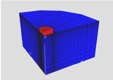
c,_ϕ soil and subjected to a central vertical load.

Fig. 1:Soil domain and mesh used in FLAC3D

Because of symmetry, only quarter of the entire soil domain of diameter 14 and R depth 5R is considered. The bottom and the outer vertical boundaries of the soil domain are far enough from the footing and thus do not disturb the soil mass in motion (i.e. velocity field) for all the soil configurations studied in this paper. A non uniform optimal mesh composed of 2420 zones is used (Figure 1). The soil region under the footing was divided horizontally into four equal angular sectors of 22.5° each and 10 rings which size gradually decreases from the centre to the periphery of the footing where very high stress gradients are developed. Beyond the footing, the soil domain was divided horizontally into four equal angular sectors of 22.5° each and into 20 rings which size increases gradually from the foundation periphery to the vertical cylindrical boundary. Vertically, the soil domain was divided into 20 zones which size decreases gradually from the bottom of the domain to the ground surface. Concerning the footing, it is subdivided horizontally into four equal angular sectors and five equal rings and vertically into one single zone. The nodes of the interface are those of the soil. Each quadrilateral element of the interface is automatically divided by FLAC3D into two triangular elements.

For the displacement boundary conditions (Figure 1), the bottom boundary was assumed to be fixed and the vertical cylindrical boundary was constrained in motion in the horizontal X and Y directions. Concerning the two symmetrical vertical planes, they were constrained in motion in the direction perpendicular to these planes.

A conventional elastic-perfectly plastic model based on the Mohr-Coulomb failure criterion is used to represent the soil. The soil elastic properties used are the shear modulus G=23MPa and the bulk modulus K ₌50MPa (for which the equivalent Young’s modulus and Poisson’s ratio are respectively E=60MPa and ν =0.3). The values of the soil shear strength parameters used in the analysis are: ϕ = 30°, ψ = 20° and c 20₌ kPa where _ψ is the soil dilation angle. The soil unit weight was taken equal to 18 kN/m3. The circular footing of radius equal to m1 and depth 0.5 m is modeled by a weightless material that follows an elastic model. The footing elastic properties used are the Young’s modulus E ₌25GPa and the Poisson’s ratio ν =0.4. Compared to the soil elastic properties, these values are well in excess of those of the soil and ensure a rigid behaviour of the footing. Notice that the soil and footing elastic properties have a negligible effect on the failure load.

X Y

The footing is connected to the soil via interface elements that follow Coulomb law. The interface is assumed to have a friction angle equal to the soil angle of internal friction and the same dilation angle and cohesion as the soil in order to simulate a perfectly rough soil-footing interface. Normal stiffness K_n =1GPa/m and shear stiffness K_s =1GPa/m are assigned to this interface.

For the computation of the ultimate bearing capacity of a rough rigid circular footing using FLAC3D, the following procedure is adopted: geostatic stresses are first applied to the soil, and then several cycles are run in order to reach a steady state of static equilibrium. Finally, the obtained displacements are set to zero in order to obtain the footing displacement due only to the footing load. In a second stage, an optimal downward vertical velocity (i.e. displacement per timestep) of _2.5×10−6_{m/timestep is}

applied to the nodes of the footing. Damping of the system is introduced by running several cycles until a steady state of plastic flow develops in the soil beneath the footing. This state is achieved when both conditions (i) a constant footing load and (ii) small values of the unbalanced forces, are satisfied as the number of cycles increases. At each cycle, the vertical footing load is obtained by using a FISH function that calculates the integral of the normal stress components for all elements in contact with the footing. The value of the vertical footing load at the plastic steady state is the ultimate footing load. The ultimate bearing capacity is then obtained by dividing this load by the footing area.

Serviceability limit state – vertical displacement

For the computation of the vertical displacement of a rigid footing under an applied vertical load, an elastic-perfectly plastic model based on the Mohr-Coulomb failure criterion is again used for the soil since it enables the development of plastic zones that may occur near the footing periphery even at small service loads and it leads to more accurate solutions than a purely elastic model. The same procedure described before concerning the geostatic stresses is used here. A uniform service stress is then applied at the base of the footing. Damping of the system is introduced by running several cycles until a steady state of static equilibrium is reached in the soil. This state is achieved when both conditions (i) a constant vertical displacement of the footing and (ii) small values of unbalanced forces, are satisfied as the number of cycles increases.

RELIABILITY ANALYSIS OF CIRCULAR FOOTINGS

The aim of this paper is to perform a reliability analysis of a circular footing resting on a

( )

c,ϕ soil and subjected to a vertical load. Two failure or unsatisfactory performance modes are considered in the analysis: the first one involves the ultimate limit state and emphasis on the ultimate bearing capacity of the footing while the second one considers the serviceability limit state and focuses on the maximal footing displacement. The two deterministic models presented in the previous section are used. The response surface methodology is used to find an approximation of the analytically-unknown performance functions. The cohesion c, the angle of internal frition _ϕ, the Young modulus E and the Poisson ratio _{ν of the soil are considered as random variables. Due to the relatively low} effect of the soil elastic properties on the ultimate bearing capacity, only c and ϕ will be considered as random variables while studying the ultimate limit state. The effect of the

uncertainty of the dilatation angle is not considered in this paper. Similarly, only the randomness of E and _{ν will be taken into consideration in the analysis of the} serviceability limit state; the soil shear strength parameters have no significant influence on the SLS. After a brief description of the performance functions used in the present analysis, the response surface methodology and its numerical implementation are presented. Then, the probabilistic numerical results based on this method are presented and discussed.

Performance functions

Two performance functions corresponding to the two unsatisfactory performance modes are used in this reliability analysis. The first one is defined with respect to the ultimate bearing capacity of the foundation. It is given as follows:

G₁ =P_u /P_S −1=F−1 (3)

where P is the ultimate foundation load calculated using FLAC_u 3D, P is the footing _s applied load and F is the safety factor. The performance function defined with respect to a prescribed admissible footing displacement is given as follows:

2 max

G =u −u (4)

where u is the vertical displacement of the footing calculated using FLAC3D under a service load P and _s u_max is the maximal admissible prescribed vertical displacement.

Response surface method

If the performance function is an explicit function of the random variables, the reliability index can be calculated easily. It should be mentioned that in FLAC3D model, the closed form solution of the performance function is not available. Thus, the determination of the reliability index is not straightforward. An algorithm based on the response surface methodology proposed by Tandjiria et al.8 is used in this paper in the aim to calculate the reliability index and the corresponding design point. The basic idea of this method is to approximate the performance function by an explicit function of the random variables, and to improve the approximation via iterations. The approximate performance function used in this study has a quadratic form. It uses a second order polynomial with squared terms but no cross terms. The expression of this approximation is given by:

( )

∑

∑

= = + + = n i i i n i i i x b x a a x G 1 2 1 0 . . (5)

where x are the random variables, _i n is the number of the random variables and

(

a ,i bi

)

are the coefficients to be determined. In this paper, two random variables are

considered for each limit state (i.e. n=2). They are characterized by their mean values

i

μ and their coefficients of variation _σi. A brief explanation of the algorithm used is as follows:

1. Evaluate the performance function G

( )

x at the mean value point _μ and at the 2n

points each at _μ±k_σ where k₌1in this paper;

2. The above 2n+1 values of G

( )

x can be used to solve equation (5) and find the coefficients

(

a ,_i b_i

)

. This gives us a tentative response surface function;

3. Solve equation (1) to obtain a tentative design point and a tentative _{β subjected to HL} the constraint that the tentative response surface function of step 2 be equal to zero; 4. Repeat steps 1 to 3 until convergence. Each time step 1 is repeated, the 2n+1

sampled points are centered at the new tentative design point of step 3.

Numerical implementation of the response surface method

As described in the previous section, determination of the Hasofer-Lind reliability index requires (i) the determination of the coefficients

(

a ,_i b_i

)

of the tentative response surface via the resolution of equation (5) for 5 sampled points and (ii) the minimization of the Hasofer-Lind reliability index subjected to the constraint that the tentative response surface function be equal to zero. These two operations constitute a single iteration and were done using the optimization toolbox available in Matlab 7.0 software. Several iterations were performed until convergence of the Hasofer-Lind reliability index. The convergence criterion considers that convergence is reached when a difference smaller than 10-2 between two successive reliability indexes is achieved. Notice that the determination of the performance function at the 5 sampled points was performed using deterministic FLAC3D calculations. The results of these computations constitute input parameters for the determination of the coefficients

(

a ,_i b_i

)

of the tentative response surface using Matlab 7.0. The value of the design point determined by the minimization procedure in Matlab 7.0 is also an input parameter for the determination of the performance function at the 5 sampled points in FLAC3D. Therefore, an exchange of data between FLAC3D and Matlab 7.0 in both directions was necessary to enable an automatic resolution of the iterative algorithm for the determination of the Hasofer-Lind reliability index. The link between FLAC3D and Matlab 7.0 was performed using text files and FISH commands.

NUMERICAL RESULTS

For the ultimate limit state, different values of the coefficients of variation of the angle of internal friction and cohesion are presented in literature. In this paper, the illustrative values used for the statistical moments of the soil shear strength parameters and their coefficient of correlation _ρc,ϕ are given as follows: μ_c =20kPa , ₌₃₀o

ϕ μ , % 20 = c

COV , COVϕ =10% and ρc,ϕ =−0.5. For the probability distribution of the

random variables, c is assumed to be log-normally distributed while _ϕ is assumed to be bounded and a beta distribution is used 2. The parameters of the beta distribution are determined from the mean value and standard deviation of _ϕ . It should be mentioned that the soil elastic properties (i.e. K and G or E and _{ν ) considered as deterministic} in the present ultimate limit state have no effect on the value of the ultimate bearing capacity. Higher values of these properties (i.e. G 100₌ MPa and K ₌200MPa) for which E = 257MPa and _{ν =}0.3, were checked. No change was observed in the value of the ultimate bearing capacity. Furthermore, a reduction by 50% in the number of cycles necessary to reach the failure was noticed (i.e. a reduction in the computation time by half).Therefore, these values will be used in all subsequent calculations when studying the ultimate limit state. The CPU time required for each simulation was found about 40 minutes on a Centrino 2.0 GHz PC.

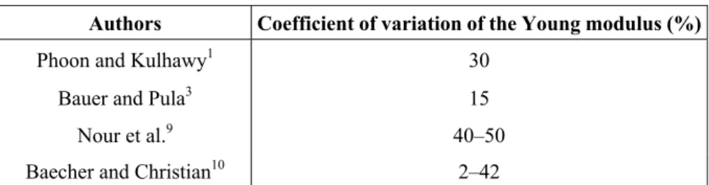
Table 1. Values of COVE as suggested by several authors

Authors Coefficient of variation of the Young modulus (%)

Phoon and Kulhawy1 ₃₀

Bauer and Pula3 ₁₅

Nour et al.9 _40–50

Baecher and Christian10 _2–42

For the serviceability limit state, soils with small values of Young modulus are used in this paper. In such soils, the variability of the compressibility characteristics is very large3_{. A lognormal distribution is used for E with a mean value of 60MPa}9_{. For the}

coefficient of variation, some values proposed and used by several authors are listed in Table 1. A value of 15% is used in this paper. Regarding the Poisson ratio, there is no available information about its random variation. Some authors have suggested that the randomness can be neglected in an analysis of settlement taking place in the case of elastic soil. Others have stated that _{ν changes within a relatively narrow interval. In this paper,} ν is considered as a lognormally distributed variable with a coefficient of variation of

%

5 . Its mean value is taken equal to 0.3. For the correlation coefficient of these two parameters, there is no information available. The results reported by some researchers 3

lead to the conclusion that this correlation is negative. In this paper, the cases of uncorrelated and correlated soil elastic properties with ρE_,υ =−0.5 are considered. The CPU time required for each serviceability limit state simulation was found about 30 minutes on a Centrino 2.0 GHz PC.

For both the ULS and SLS, the dilation angle was held constant and equal to 20°. Higher values of this parameter lead to a greater bearing capacity and a smaller footing displacement due to an applied footing load. Hence, for both limit states, higher values of the reliability index would be obtained for a greater value of the soil dilation.

Ultimate limit state

The convergence criterion of the ultimate limit state was reached after only 5 iterations. Thus, only 25 numerical simulations using FLAC3D were necessary.

Reliability index and design point

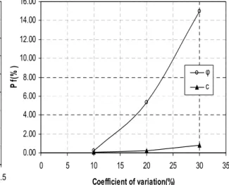
Figure (2a) presents the Hasofer-Lind reliability index versus the safety factor F=Pu/Ps.

Both correlated and uncorrelated shear strength parameters are considered. The reliability index increases with the increase of the safety factor. The comparison of the results of correlated variables with those of uncorrelated variables shows that the reliability index corresponding to uncorrelated variables is smaller than the one of negatively correlated variables. One can conclude that the hypothesis of uncorrelated shear strength parameters is conservative and non-economic in comparison to the one of negatively correlated parameters. For instance, when the safety factor is equal to 3.15, the reliability index increases by 35% if the variables c and _ϕ are considered as negatively correlated.

Sensitivity of failure probability to the variability of the soil shear strength parameters To study the effect of the variability of the soil shear strength on the failure probability, Figure (2b) shows the failure probability versus the coefficient of variation of c and _ϕ

for negatively correlated variables. The value of the safety factor is taken equal to 3.15. For each curve, the coefficient of variation of a parameter is hold to the same constant value given before and the coefficient of variation of the second parameter is varied over the range 10–30%.

The results show that the failure probability is highly influenced by the coefficient of variation of the angle of internal friction, the greater the scatter in ϕ the higher the failure probability of the foundation. This means that the accurate determination of the distribution of this parameter is very important in obtaining reliable probabilistic results. In contrast, the coefficient of variation of c does not significantly affect the failure probability. 0 0.5 1 1.5 2 2.5 3 3.5 4 4.5 1.0 1.5 2.0 2.5 3.0 3.5 F β HL ρc,φ= 0 ρc,φ= -0.5 0.00 2.00 4.00 6.00 8.00 10.00 12.00 14.00 16.00 0 5 10 15 20 25 30 35 Coefficient of variation(%) Pf (% ) φ c

Fig. 2: (a) Reliability index versus safety factor

F=Pu/Ps.

(b) Effect of the variability of cand ϕ on the failure probability.

Serviceability limit state

Reliability index and design point

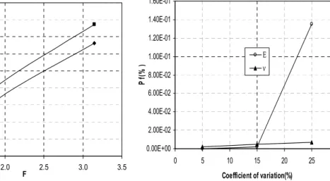
The threshold value of the settlement adopted in this paper is umax= 0.1 m. Figure (3a)

presents the Hasofer-Lind reliability index versus the safety factor F=Pu/Ps where Pu in

this figure is taken as in the ULS as the footing load that leads to bearing failure. Notice however that the ultimate load leading to an unsatisfactory performance mode in the SLS is the one corresponding to the maximal displacement of 0.1 m. The corresponding stress is 1640 kN/m2. Both correlated and uncorrelated soil elastic properties are considered.

The same conclusion drawn in the ultimate limit state remains valid here, i.e. the reliability index corresponding to uncorrelated variables is smaller than the one of negatively correlated variables. By comparing Figure (3a) with Figure (2a), one can notice that for values of the safety factor of about 3.0 (i.e. for practical values of the safety factor), the reliability index of the ultimate limit state is significantly smaller than that of the serviceability limit state. Thus, for these values of the safety factor, the ultimate limit state is predominant and will have the highest contribution in the determination of the system failure probability as it will be seen in the section entitled ‘System failure probability’. The difference between the reliability indexes of the two limit states becomes smaller for smaller values of the safety factor. Consequently, when the safety factor decreases, the two limit states (i.e. the ultimate and the serviceability

ones) have approximately similar contribution in the computation of the system failure probability (see again the section entitled ‘System failure probability’).

0.0 1.0 2.0 3.0 4.0 5.0 6.0 7.0 8.0 9.0 1.0 1.5 2.0 2.5 3.0 3.5 F β HL ρE,ν = 0 ρE,ν = -0.5 0.00E+00 2.00E-02 4.00E-02 6.00E-02 8.00E-02 1.00E-01 1.20E-01 1.40E-01 1.60E-01 0 5 10 15 20 25 30 Coefficient of variation(%) Pf (% ) Ε_ν

Fig. 3: (a) Reliability index versus safety factor F = Pu/Ps for the SLS.

(b) Effect of the variability of E and ν on the failure probability.

Sensitivity of failure probability to the variability of the soil elastic properties

As for the ultimate limit state, Figure (3b) shows the FORM failure probability versus the coefficient of variation of E and υ for negatively correlated variables. A vertical stress of 1000 kN/m2 is applied to the footing. For each curve, the coefficient of variation of a parameter is hold to the same constant value given before and the coefficient of variation of the second parameter is varied over the range 5–25%. The results show that the failure probability of the serviceability limit state is highly influenced by the coefficient of variation of the Young modulus, the greater the scatter in E the higher the failure probability of the foundation. This means that the accurate determination of the distribution of this parameter is very important in obtaining reliable probabilistic results.

System failure probability

The system failure probability under the two limit states involving the ultimate and the serviceability limit states of the footing is given by:

(

U S

)

P

( )

U P

( )

S P

(

U S

)

P

P_{f f f f f}

sys = ∪ = + − ∩ (5)

where Pf(U) is the failure probability under only the ultimate limit state, Pf(S) is the failure probability under only the serviceability limit state and Pf(U∩S) is the failure probability under the ultimate and the serviceability limit states.

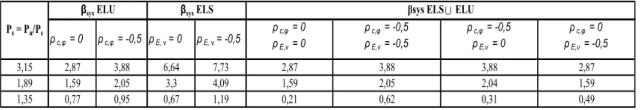
For different values of the safety factor defined against bearing capacity failure, Table 2 presents the system reliability index defined as:

( )

1

sys Pf sys

Table 2. System reliability index versus safety factor F=Pu/Ps ρc,φ = 0 ρc,φ = -0,5 ρE, ν = 0 ρE, ν = -0,5 ρc,φ= 0 ρE,ν = 0 ρc,φ= -0,5 ρE,ν = -0,5 ρc,φ= -0,5 ρE,ν = 0 ρc,φ = 0 ρE,ν = -0,5 3,15 2,87 3,88 6,64 7,73 2,87 3,88 3,88 2,87 1,89 1,59 2,05 3,3 4,09 1,59 2,05 2,04 1,59 1,35 0,77 0,95 0,67 1,19 0,21 0,62 0,31 0,49 Ps = Pu/Ps

β_sys ELU β_sys ELS βsys ELS ELUU

Four cases are considered: they are the combinations of correlated and uncorrelated shear strength parameters with correlated and uncorrelated soil elastic properties. It can be seen from this table that for the system reliability, the assumption of uncorrelated parameters is conservative in comparison to the one of negatively correlated variables. For practical values of the safety factor (i.e. about 3.0), where the ultimate limit state is predominant, one can notice that the system reliability index is equal to that of the ultimate limit state. When the safety factor decreases, the system reliability depends on both limit states and a smaller reliability index than the one corresponding to a single limit state was found. As a conclusion, both limit states have to be considered in the reliability analysis of foundations for small values of the safety factor.

CONCLUSIONS

A reliability-based analysis of a circular footing resting on a c-ϕ soil is presented. Both ultimate and serviceability limit states are considered. The deterministic models used are based on numerical simulations using FLAC3D_{. The Hasofer-Lind reliability index is}

adopted here for the assessment of the foundation reliability. The response surface methodology is used to find an approximation of the analytically-unknown limit state surfaces and the corresponding reliability indexes. The main conclusions of this paper can be summarized as follows:

• The hypothesis of uncorrelated parameters was found conservative in comparison to the one of negatively correlated variables and leads to non-economic design; • The failure probability was found highly influenced by the uncertainties of the

angle of internal friction for the ultimate limit state and by the uncertainties of the Young modulus for the serviceability limit state;

• For practical values of the safety factor (i.e. close to 3.0), the ultimate limit state was predominant. The corresponding system reliability index was found equal to that of the ultimate limit state. For smaller values of the safety factor (which correspond to no practical cases), the system reliability depends on both limit states and a smaller reliability index than the one corresponding to a single limit state, was found. Thus, both limit states have to be considered in the reliability analysis of foundations for small values of the safety factor.

REFERENCES

1. Phoon, K.-K. and Kulhawy, F.H. 1999. Evaluation of geotechnical property variability. Can. Geotech. J., 36:625–39.

2. Fenton, G.A. and Griffiths, D.V. 2003. Bearing capacity prediction of spatially random c-φ soils. Can. Geotech. J., 40:54–65.

3. Bauer, J. and Pula, W. 2000. Reliability with respect to settlement limit-states of shallow foundations on linearly-deformable subsoil. Computers and Geotechnics, 26:281–308.

4. Youssef Abdel Massih, D.S., Soubra, A.-H. and Low, B.K. 2007. Reliability-based analysis and design of strip footings against bearing capacity failure. J. of Geotech. and Geoenv. Engrg., ASCE, in press.

5. Hasofer, A. M. and Lind, N. C. 1974. Exact and invariant second-moment code format. J. of Engrg. Mech., ASCE, 100(1):11–121.

6. Low, B. K. and Tang, W. H. 1997. Efficient reliability evaluation using spreadsheet. J. of Engrg. Mech., ASCE, 123:749–52.

7. Low, B. K. 2005. Reliability-based design applied to retaining walls. Géotechnique, 55(1):63–75.

8. Tandjiria, V., Teh, C.I. and Low, B.K. 2000. Reliability analysis of laterally loaded piles using response surface methods. Structural Safety, 22:335–55.

9. Nour, A., Slimani, A. and Laouami N. 2002. Foundation settlement statistics via finite element analysis. Computers & Geotechnics, 29:641–672

10. Baecher, G. and Christian, J. 2003. Reliability and Statistics in Geotechnical Engineering. Wiley, England, 605p.