Calculation of river sediment fluxes from uncertain and infrequent measurements

HAL Id: hal-01098277

https://hal.archives-ouvertes.fr/hal-01098277

Submitted on 23 Dec 2014

HAL is a multi-disciplinary open access

archive for the deposit and dissemination of sci-entific research documents, whether they are pub-lished or not. The documents may come from teaching and research institutions in France or abroad, or from public or private research centers.

L’archive ouverte pluridisciplinaire HAL, est destinée au dépôt et à la diffusion de documents scientifiques de niveau recherche, publiés ou non, émanant des établissements d’enseignement et de recherche français ou étrangers, des laboratoires publics ou privés.

B. Cheviron, Magalie Delmas, Olivier Cerdan, J.M. Mouchel

To cite this version:

B. Cheviron, Magalie Delmas, Olivier Cerdan, J.M. Mouchel. Calculation of river sediment fluxes from uncertain and infrequent measurements. Journal of Hydrology, Elsevier, 2014, 508, pp.364-373. �10.1016/j.jhydrol.2013.10.057�. �hal-01098277�

Calculation of river sediment fluxes from uncertain and infrequent measurements

1 2

Bruno Cheviron1,*, Magalie Delmas2, Olivier Cerdan3 & Jean-Marie Mouchel4 3

4

1: UMR G-EAU, IRSTEA, 361 rue Jean-François Breton, 34196 Montpellier Cedex 05, France - 5

bruno.cheviron@irstea.fr 6

2: UMR LISAH, INRA, 2 place Pierre Viala, 34060 Montpellier Cedex 01, France -7

magalie.delmas@supagro.inra.fr 8

3: BRGM, 3 avenue Claude Guillemin, BP6009, 45060 Orléans Cedex 2, France - o.cerdan@brgm.fr 9

4: UMR SISYPHE, Université Paris VI-Pierre et Marie Curie, 4 place Jussieu, 75252 Paris Cedex 05, 10

France - jean-marie.mouchel@upmc.fr 11

* corresponding author, tel: +33 (00) 4 67 04 63 64 12

13

Keywords: River flow, sediment transport, uncertainty analysis, rating curves. 14

Abstract

15 16

This paper addresses feasibility issues in the calculation of fluxes of suspended particulate matter 17

(SPM) from degraded-quality data for flow discharge (Q) and sediment concentration (C) under the 18

additional constraints of infrequent and irregular sediment concentration samplings. A crucial setting 19

of the scope involves establishing the number of data required to counterbalance limitations in the 20

measurement accuracy and frequency of data collection. This study also compares the merits and 21

drawbacks of the classical rating curve (C=aQb) with those of an improved rating curve approach 22

(IRCA: C=aQb+a1S) in which the correction term is an indicator of the variations in sediment storage, 23

thus relating it to flow dynamics. This alternative formulation remedies the known systematic 24

underestimations in the classical rating curve and correctly resists the degradation in data quality and 25

availability, as shown in a series of problematic though realistic cases. For example, monthly 26

concentration samplings (in average) with a random relative error in the [-30%, +30%] range 27

combined with daily discharge records with a systematic relative error in the [-5%, +5%] range still 28

yield SPM fluxes within factors of 0.60-1.65 of the real value, provided that 15 years of data are 29

available. A shorter 5-day time interval (on average) between samplings lowers the relative error in 30

the SPM fluxes to below 10%, a result directly related to the increased number of Q-C pairs available 31

for fitting. For regional-scale applications, this study may be used to define the data quality level

32

(uncertainty, frequency and/or number) compatible with reliable computation of river sediment

33

fluxes. Provided that at least 200 concentration samplings are available, the use of a sediment rating

34

curve model augmented to account for storage effects fulfils this purpose with satisfactory accuracy

35

under real-life conditions. 36

1. Introduction

38 39

Sediment fluxes in fluvial systems reflect the denudation processes that occur on the earth’s surface 40

and exert a controlling effect on the fates of nutrients, organic pollutants and heavy metals. 41

Therefore, assessment of sediment fluxes aids in characterising the impact of particulate transfer on 42

water quality throughout the river system. However, the estimation of realistic sediment budgets 43

requires long-term discharge-concentration data (Walling and Webb 1985, Ludwig and Probst 1998, 44

Webb et al. 2003, Delmas et al. 2009), which often suffer from poor availability and reliability 45

(Meybeck et al. 2003, Walling and Fang 2003). In particular, uncertainties in both the sampling and 46

calculation methods affect the measurement of sediment concentration (SPM) fluxes (Rode and Surh 47

2007). Moreover, significant drifts in the measured quantities may arise due to the location of the 48

sampling in the river section because the suspended sediment concentration varies within cross-49

sections of the rivers, thus necessitating a series of depth- and width-integrated measurements 50

(Horowitz, 1997). However, in most cases, modellers and decision-makers use the daily discharge 51

records combined with infrequent sediment concentration samplings, which are generally collected 52

at a single location and exhibit high temporal variability. 53

54

Previous studies have indicated how increased sampling frequencies and total periods of data 55

collection can reduce uncertainties in the predicted SPM or trace element fluxes (Horowitz et al.

56

2001, Coynel et al. 2004, Moatar and Meybeck 2005, Rode and Surh, 2007), but a complementary 57

and perhaps broader strategy would involve treatment of the analysis in terms of the interactions 58

between the number of data, the time interval between samplings (affected by a realistic random 59

component) and the total period of the data collection. This analysis would be particularly pertinent 60

in the numerous areas where available the sediment concentration data are by-products of programs 61

for water quality monitoring that involve infrequent (approximately monthly) sampling (Delmas et al. 62

2012). A relevant and widely used methodology is the reconstruction of continuous (daily) 63

fluctuations in the sediment concentration from the empirical relationships (C(Q) rating curves) that 64

link the sediment concentration (C) to the water discharge (Q) values. The classical C(Q)=aQb rating 65

curve is often used for this purpose. Nevertheless, for sediment transport studies, the occasional 66

strong non-linearity in the C(Q) relationship and the presence of only a few extreme events point to 67

well known and problematic cases when fitting power laws (Laherrere 1996, Goldstein et al. 2004). 68

These problematic cases suggest the use of truncated intervals of Q values (Moatar et al. 2012) or 69

data subdivision and hypothesising of the distinct C(Q) relationships with the seasons, basin sizes or 70

properties (Walling and Webb 1981, Smart et al. 1999, Quilbé et al. 2006; Delmas et al. 2009). 71

Another possibility is the addition of correction terms (Laherrere and Sornette 1998) with a user-72

defined physical meaning. Ferguson (1986, 1987) chose the latter option in his inaugural papers that 73

tackled the advantages and limitations in estimating sediment fluxes from power-law rating curves. 74

Similar to other research domains, an open question is whether to attribute a deterministic physical 75

meaning to the pre-factor and the exponent (Peters-Kümmerly 1973, Morgan 1995, Asselmann 2000) 76

or to consider them as conceptually imperfect though demonstrably statistically relevant. Addressing 77

these questions with a clear physical sense opens the door for a wide series of improved rating 78

curves and variants, as advocated by Phillips et al. (1999), Asselmann (2000), Horowitz (2003) and 79

Delmas et al. (2011), among others. For example, Picouet et al. (2001) hypothesised two sediment

80

sources (bank and hillslope erosion), and Mano et al. (2009) introduced explicit climatic and

81

topographic factors.

82 83

The objective of the current paper is to address the precision and sensitivity issues that exist in 84

prediction of SPM fluxes for typical cases with data of degraded-quality gathered from infrequent 85

samplings. We consider the C and Q measurements to be affected by errors of different types and 86

magnitudes. As commonly reported, we hypothesised a higher probability of error for concentration 87

than for discharge measurements. Concentration data were considered prone to random errors in a 88

[-30%, +30%] interval around the measured values, whereas five systematic biases were tested for 89

discharge data in the [-20%, 20%] interval around the daily records. Moreover, infrequent 90

concentration measurements were simulated together with slightly perturbed sampling periods. The 91

framework of this study compares the merits and drawbacks of the classical rating curve with those 92

of an improved rating curve approach. The latter includes a correction term as an indicator of 93

sediment storage, thus relating the variation to flow dynamics. This work relies on a USGS dataset 94

encompassing multiple rivers, basin typologies and years. 95

96

2. Material & Methods

97 98

2.1 Database 99

100

The present study relies on daily discharge-concentration data collected over several years at 22 101

USGS stations taken from the larger dataset available at http://waterdata.usgs.gov/. The selected 102

stations cover a wide range of river basin typologies and sizes and are associated with specific 103

discharge and SPM statistics (Table 1). For the Des Moines River station, we chose to split the records 104

into two distinct periods because we observed notably large discharge variations over the first years 105

of data collection (1961-1977) followed by rather limited variation over the most recent years (1977-106

2004). Several stations display notably low water levels and even close to intermittent flows under 107

severe winter conditions (e.g., station 21, Salinas River near Spreckels), summer droughts (e.g., 108

station 18, Kaskaskia River at Cook Mills) or both (e.g., station 7, Hocking River at Athens). However,

109

stations in the USGS database that exhibit complete drying or glaciations have been discarded from

110

the analysis because they require different treatment. This choice tends to omit basins with small

111

drainage areas, especially those that experience sharp climatic conditions. Nevertheless, various 112

temperate to continental climates are accounted for at stations in California (CA), Illinois (IL), Iowa 113

(IA), Missouri (MI), North Carolina (NC), Ohio (OH) and Virginia (VA). Another merit of sufficiently

114

large basins for the present study is response times that are greater than the reference daily

sampling period for the discharge and concentration measurements. In addition to the temporal

116

arguments, large basins are also more integrative than smaller basins because they offer additional

117

spatial variability with respect to the sediment sources and delivery processes combined with larger

118

climatic variability.

119 120

[TABLE 1 ABOUT HERE] 121

122

2.2 Rating curves 123

124

In addition to the classical C=aQb rating curve (RC), different expressions and strategies have been 125

tested and described in detail by Delmas et al. (2011). Among these, emphasis is placed in this work 126

on the Improved Rating Curve Approach (IRCA), which hypothesises C=aQb+a1S, where a1 is a 127

parameter, S is the sediment storage index and S is the daily variation. This method operates in two 128

steps. First, the method fits the C=aQb model, thus freezing the a and b coefficients, and 129

subsequently fits the a1 parameter, which is the only remaining degree of freedom in the a1S 130

correction term. The IRCA was implemented to remedy the known limitations of the RC, especially its 131

inability to include flow dynamics or antecedent flow conditions in the prediction of C values. 132

133

For this purpose, the sediment storage index is described as a function of discharge dynamics: 134

 

where A is a dimensionless coefficient that controls the amplitude of S variations, and q(t) is the 135

instantaneous Q(t) value on the rising limbs of the hydrograph or a sliding average of Q(t) values on 136

the falling limbs. This double status of q(t) ensures asymmetry between quick sediment loading and 137

delayed sediment storage, which is the working hypothesis that underlies the IRCA. The sliding 138

average extends itself backwards in time towards the beginning of the current falling limb but is 139

limited to 20 days at most, which is the chosen approach used to account for antecedent flow 140

conditions. 141

142

The IRCA also requires statistical analysis to establish the upper limit of the base flow, given as Q0. 143

From the adopted assumptions, S varies between 0 for extreme discharges (all possible sediments 144

present in the flow) and 1 when flow ceases (all material stored and available). The choice of A=0.1 145

yields S=0.95, 0.75, 0.50, 0.25 and 0.05 for q/Q0 ratios of approximately 0.5, 3, 7, 14 and 30, 146

respectively. This choice also implies that S0.9 for q=Q0, and thus the sedi e t a aila ilit ould 147

be approximately 90%. 148

149

Figure 1 shows the variations in the sediment storage index in an application to the Hocking River at 150

Athens (station 7, Table 1). The figure displays the main characteristics of this approach: asymmetry 151

between the delayed sediment storage and quick sediment mobilisation, damping of the high-152

frequency oscillations and maximum sediment storage associated with long-lasting low discharges. 153

The intent of the IRCA is to use the daily variations of the sediment storage index as relevant 154

information for the flow dynamics, as handled by the a1S correction term in the C=aQ b

+a1S model. 155

156

[FIGURE 1 ABOUT HERE] 157

158

In a strict sense, both the C=aQb+a1S and C=aQ b

+a1S expressions should be considered in this work

159

as odels and ot la s . La s should be written with an additional explicit error term, either

160

multiplicative or additive, whose distribution should be assessed from the characteristics and is

161

missing in the data (Q, C) measurements. This option would take into account that the C=aQb and

162

C=aQb+a1S expressions are exact formulations of the problem, attributing the deviations between

163

the calculated and observed quantities to variations in the associated error terms. Instead, the

164

current option views the C=aQb and C=aQb+a1S expressions as imperfect models with inherent

errors. Therefore, the scope of this work focuses on the dispersion of the model predictions with

166

alterations of the (Q, C) dataset.

167 168 2.3 Fitting procedures 169 170

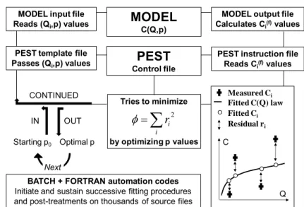
All fittings were automated using a multi-stage procedure centred on the PEST parameter estimation 171

software (Doherty, 2004) but also resorted to further programming. Figure 2 displays the simplified 172

flow chart, which is briefly described. The user selects a C(Q) model with p parameters to fit, entering 173

the flow chart with the initial p0 vector of parameter values and also providing a series of Qi 174

discharge samplings. This (Qi, p) set is processed via a p og a that al ulates the fitted Ci

(f)

value 175

associated with each Qi value for the selected power law. Next, PEST carries out an overall 176

optimisation based on the minimisation of an objective function, which is calculated as the sum of 177

the squared residuals between the observed Ci values and the fitted Ci

(f)

values. Once the 178

optimisation has been completed, PEST estimates the goodness-of-fit by calculating the coefficient of 179

determination, known as R. The R value may therefore be used for comparisons between fittings. 180

One of the interesting features in PEST is its ability to handle power laws with or without log

181

transformations, and the choice is left to the use ’s dis etio . “lightl ette esults ha e ee

182

obtained in this work by fitting the untransformed expressions. 183

184

[FIGURE 2 ABOUT HERE] 185

186

2.4 Methods for calculating fluxes and errors 187

188

The real amount of exported sediment in the [0, T] total time period is the unknown SPM flux: 189

   





dt

t

C

t

Q

F

where Q is the discharge, C is the concentration of suspended particulate matter (SPM) and t is time. 190

191

The straightforward approximation for direct calculation of F is: 192 i i N i i N

Q

C

t

F







where Qi and Ci are time-averaged values over the ti intervals covering the [0, T] time period. 193

194

The discrepancy between F and FN plausibly increases with increased ti values. Nevertheless, certain 195

rare and fortuitous combinations of large ti values may still lead to FN  F, from compensating 196

effects between the underestimations and overestimations of SPM fluxes over certain periods. 197

Therefore, the gap between FN and F is not expected to vary in any monotonous or linear manner 198

with increasing ti values. By contrast, the ti intervals that are smaller than the characteristic time 199

period of fluctuations in Q and C values tend to ensure the reliability of the FN approximation. 200

Because the SPM regimes are related to the basin sizes (Meybeck et al. 2003) and only drainage 201

areas larger than 1000 km2 are considered in this work, the FN fluxes calculated from the error-free 202

daily discharge and concentration records are considered as exact solutions (FN  F) in the following. 203

The subsequent developments aim to test the deviations from this best-case scenario that appear 204

when coping with infrequent and/or uncertain data (i.e., random errors in the concentration data 205

and systematic errors in the discharge data and sparse concentration samplings in this work). 206

207

The missing concentration data in [3] may be replaced by concentration values obtained from the 208

fitted C(Q) models. Each Qi datum results in a predicted Ci

(f)

concentration value, and the exported 209

SPM flux now can be approximated by: 210 i f i N i i f N QC t F, 





The hypothesis for the missing C data implies that only n<N values have been measured. In the 212

calculation of FN,f, one may either use the available concentration data Ci instead of the fitted values 213

or systematically resort to the entire series of Ci

(f)

values, as in this study. 214

215

From a theoretical point of view, any given Ci

(f)

is an unknown function of the entire dataset via the 216 fitting procedure: 217





C

Q

Q

C

C

C

t

t

t

C



, . . . ,

,

, . . . ,

, . . . ,

,



, . . . ,



, . . . ,



with irregular tk intervals between successive C samplings in the general case. 218

219

For regular t intervals between concentration samplings, the (t1,…,tk,…,tn) temporal argument 220

could be reduced to (t, n) or (t, T) without any additional loss of information. Combining these 221

elements with shortened notations Q’=(Q1,…,QN) and C’=(C1,…,Cn) would yield: 222





The assessment of SPM fluxes (FN,f) from the source data (Q’, C’) under experimental conditions (t, 224

T) is a two-stage process that first solves the inverse problem by fitting the optimal {p} parameter set 225

in the C(Q) model (rating curve) and subsequently uses it for direct calculations by means of [4]: 226



  

Most of the time, at least in the French river surveillance network, the intervals between C samplings 227

are only approximately regular such that t~ should be used instead of t. The present procedure is

228

assumed to be valid if the average of the t~ values over the data collection period remains

229

sufficiently close to t. In other words, this hypothesis is intended to authorise random fluctuations

230

of t~ around t=T/n and is not assumed to hold for drastic changes in data collection strategy.

231 232

The objective of Step 1 is to test the combined effects of systematic biases in Q’ with random errors 233

on C’, thus maintaining the optimal conditions of data collection: daily discharge and concentration 234

data over several years. Emphasis is placed on the effects of degraded data quality on both the fitted 235

parameters and the estimated SPM fluxes for the classical (C=aQb) and improved (C=aQb+a1S) rating 236

curves. 237

238

Five systematic relative errors in the discharge measurements are addressed and are noted as Qr = -239

20%, -10%, 0%, +10% and +20%: if Q* is the measured dataset and Q’ is the collection of exact 240

values, the listed Qr cases are also written as Q*/Q’=0.8, 0.9, 1.0, 1.1 and 1.2, respectively. However, 241

random relative errors in the concentration measurements (CR) were assumed as uniformly 242

distributed within the [-30%, +30%] interval around the collected data. This random treatment 243

involved replicating each station in Table 1 into 100 virtual stations with the intended perturbations 244

in the C data. 245

246

The selected objectives are to study the relative variations of the parameters {pr} and those of the 247

calculated SPM fluxes. The latter appear in more eloquent representations when displaying the ratios 248

of calculated and exact fluxes such that the stages of the test procedure may be summarised in: 249





 

where the expected results are the mean variation trends in function of Qr values with dispersion 250

effects arising from the randomised CR concentration data. The {pr} set is {ar, br} for the classical 251

rating curve and {ar, br, a1r} for the IRCA. 252

253

Step 2 focuses on the effects of the sampling frequencies, especially those with increasing time 254

intervals between C data, while ensuring that the data quality is unaffected, thus producing error-255

free Q and C data. Numerous combinations of (tR, TC) values have been tested, where t R 256

designates an average sampling interval affected by a s all a do pe tu atio (at ost e ual to 257

t/2), and TC is the total period of data collection. The t R

treatment is the approach chosen to 258

account for the irregular t~ intervals previously mentioned. The targets are once again the relative 259

variations and dispersions of the SPM fluxes, as shown in the ratios of calculated and exact fluxes: 260





t

,

T





F

F

261

Step 3 analyses the combined effects of the degraded Q-C data quality and infrequent C 262

measurements on the calculated SPM fluxes within the following procedure: 263





264

Finally, step 4 provides an application of the IRCA around the estimation of SPM exports from French 265

rivers to the sea. Contrary to the preceding sections, F is unknown and is thus estimated from 266

confidence intervals around the F/FN,f ratios by relying on the calculated FN,f fluxes. 267

268 269

3. Results and discussion

270 271

3.1 Step 1: Effects of data uncertainty on the calculated SPM fluxes 272

273

Effects of data uncertainty on the fitted parameters 274

275

Theoretical predictions are available from the scale-invariant properties of the C=aQb law: the law

276

should still hold with a modified pre-factor (a* instead of a) and unchanged exponent (b) when 277

modifying the argument, i.e., measuring Q* instead of the real Q value: 278 b b b Q a Q Q Q a aQ C * * * *        [11] with a*=a(Q/Q*)b. 279 280

For example, the underestimation of Q by 20% (Qr = -20%) corresponds to Q*/Q = 0.8, thus Q/Q* = 281

1.25 and a*/a = (1.25)b. A numerical application with a typical b value of 0.85 yields a*/a=1.21. In 282

such a case, a relative variation ar = +21% is theoretically expected. Similar predictions are available 283

for the other tested Qr values and are ep ese ted the Theo dotted li es i Figu e . Because 284

the b exponent is supposedly unaffected, its relative variation br should be zero. No such prediction is 285

available for a1 and a1r. 286

287

[FIGURE 3 ABOUT HERE] 288

289

Figure 3 gathers the ar, br and a1r variations; the latter is specific to the C=aQ b

+a1S model, and the 290

former two are common with the C=aQbmodel. All curves display the global averages of ar, br or a1r 291

for the 22 stations listed in Table 1, and each one is replicated into 100 virtual stations to satisfy the 292

random procedure on C data. Taking the example of ar, the upper (+) and lower (-) limits of the 293

dispersion envelope are plotted as: 294

 

 

   

_a

 

Q

Q

a

a

Q

Q

a

Q

a

₁

_.

_{7 3}

7 3

.

1

*













where a* is the standard deviation in the a* values and all quantities are functions of Qr except a, 295

which is the reference value obtained for Qr = 0. The a*/a term is a normalised standard deviation. 296

297

The 1.73 factor is usually associated with a 100%-confidence interval for uniform random 298

distributions: once the average value (AV) and standard deviation () are known, the real value falls 299

in the [AV-1.73 AV+1.73 ] interval. In this work, the uniform random distribution CR results in 300

nearly uniform random distributions of a*(Qr,C R

) and ar(Qr,C R

) values for each Qr value, thus ensuring 301

the validity of the calculated dispersion envelope for ar(Qr,C R

). The same procedure applies to 302

parameters b and a1. 303

304

Figures 3a, d and g examine the ar(Qr) trends and compare them with the theoretical predictions for 305

increasing values of the PEST coefficient of determination (R). The atypical non-monotonous 306

variation displayed in Figure 3a is essentially due to poorly fitted data (R0.2) from stations 14, 16, 18 307

and 19 in Table 1. At such low R values, equifinality unavoidably exists such that completely different 308

(a, b) couples lead to similar performances in the optimisation. For the cited stations, unexpectedly 309

high a values compensate for the effects of notably low b<<1 values, yielding R values otherwise 310

obtained from (a, b) couples with b1. 311

312

In Figure 3a, d and g, the dispersion decreases with increasing R values and remains limited in the 313

sense that variability is explained by the ar(Qr) trends rather tha the o thogo al dispe si e 314

random effects. As expected, the ar(Qr) curves best match the theoretical curves for increasing R 315

values, which indicate a clearer power-law organisation of the dataset. Unfortunately, only 7 stations 316

are encompassed by the R>0.65 criteria vs. 17 stations out of 22 for R>0.3. 317

318

Rather weak dispersions and low br values (i.e., nearly unchanged b exponents) in Figure 3b, e, and h 319

appear to be in good agreement with expectations arising from the scale-invariance properties of 320

power laws. However, a striking feature is the increasing variability of ar and br with decreasing 321

determination values. The underlying and unanswered question at this point is whether this 322

variability will endanger the reliability of SPM flux calculations for fittings with low determination 323

values. This question is the subject of the ad o ated o posite a al sis performed in the following 324

paragraphs, from data uncertainty to uncertainty in the fitted parameters as well as in the calculated 325

fluxes. 326

327

The a1r variations (Figure 3c, f and i) also show limited dispersion, except for strong discharge 328

underestimations. Positive relative errors in the discharge (Qr>0) cause positive relative variations in 329

the a1 coefficient (a1r>0). A key point is that the S term is identical regardless of the Qr value 330

because the q/Q0 ratio is used in [1], where both q and Q0 are affected by the same relative error in 331

the discharge values. This choice of S, referred to as ide ti al o st u tio , allows direct 332

interpretation of the role played by a1: the a1S correction behaves similar to a1, producing its 333

strongest relative variations (a1r=-30%) for the strongest discharge underestimations (Qr=-20%). 334

335

Effects of data uncertainty on the calculated SPM fluxes 336

337

Contrary to the fitted coefficients, the calculated SPM fluxes exhibit almost no dependence on the 338

determination (R) values. Therefore, Figure 4 plots the SPM fluxes and dispersions obtained for all R 339

values. As shown previously, the upper (+) and lower (-) limits of the dispersion envelope are written: 340

 

 

 

 

_F

 

Q

Q

F

F

F

Q

Q

F

Q

F

F

7 3

.

1

7 3

.

1





























[FIGURE 4 ABOUT HERE] 342

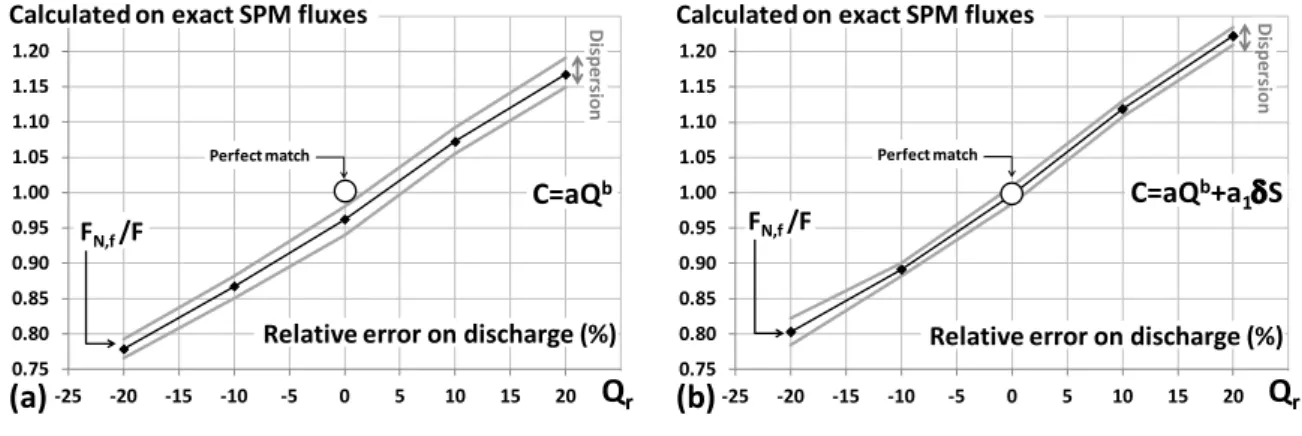
343

Figure 4a and b show weak dispersions and similar variation trends because the calculated SPM 344

fluxes increase with the estimated discharge values. The relative variations in the calculated fluxes 345

are near-linear functions of the systematic relative error present in the discharge measurements for 346

both the classical C=aQb (Figure 4a) and the improved C=aQb+a1S (Figure 4b) rating curves. The 347

difference et ee these pa allel u es is the offset added i Figu e the a1S correction, 348

which perfectly remedies the underestimation due to the classical method. The gain obtained from 349

the a1S o e tio is app o i atel % alo g the al ulated on e a t e ti al a is, ith e e 350

weaker dispersion in the results. For example, if the discharge is known with a 10% uncertainty (5% 351

on each side of the Qr=0 line), then FN,f/F lies within the 0.88-1.04 and 0.93-1.07 ranges of the 352

classical and improved rating curves, respectively. 353

354

Looking at the nearly stable b values (br 0 in Figure 3b, e and h), it is worth noting that increases in 355

the fitted a values (ar > 0 in Figure 3d and g) were not sufficient to counterbalance the influence of 356

the discharge underestimations (Qr < 0). The calculated fluxes still underestimate the real values 357

when the discharge is underestimated for both methods in Figure 4. However, the overall effect of 358

the storage term is an increase in the calculated (FN,f) SPM fluxes, which is validated by 359

improvements of approximately 5% in the determination values. 360

361

3.2 Step 2: Effects of data infrequence on the calculated SPM fluxes 362

This subsection leaves data quality concerns aside to focus on data availability, especially on the 364

problem of infrequent C data. This subsection also tackles the sampling frequency issue by 365

addressing the interplay between the number (n) of available data, the total collection period (T) and 366

the sampling period (t), as commented next to [6]. As previously mentioned, the sampling periods 367

have always been tested with slight random perturbations (tR) of the predefined values to account 368

for more realistic field conditions, resulting in approximations (t~) of the predefined t intervals. 369

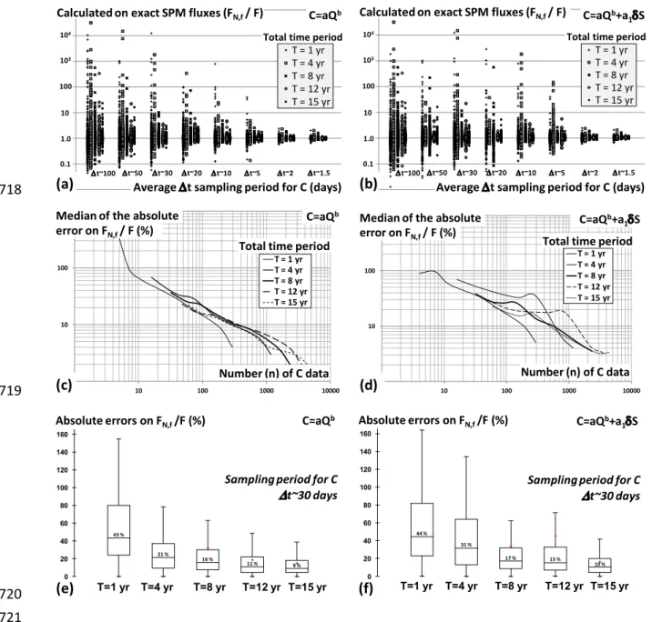
Figure 5 displays the ratio of the calculated and exact SPM fluxes, the medians of the absolute errors 370

on this ratio and the statistics for the absolute errors on this ratio in the t~30 day case for various 371

(n, T, t) triplets, thus allowing comparisons between the fitted C=aQb and C=aQb+a1S models. 372

373

[FIGURE 5 ABOUT HERE] 374

375

Figure 5a targets the evolution of the calculated on exact ratios of SPM fluxes for decreasing values 376

of the sampling interval (t) and also shows the positive impact of increasingly long periods of data 377

collection (T) for the given sampling intervals. A clear increase in dispersion occurs for t>5 days 378

combined with T<4 years. Further on the left of the diagram, the rather typical monthly sampling 379

period (t~30 days) requires at least an 8-year collection period (T=8 years) for the calculated on 380

exact ratios to lie within the gross [0.5, 5.0] interval. Figure 5b also begins with highly dispersed 381

values for combinations of high sampling periods, even with long collection periods, and exhibits 382

additional oscillations before achieving convergence because it is obviously more seriously affected 383

by weak T values. The main difference is the highest dispersion for t~5 days and T=4 years and for 384

t~20 days and T=8 years. A common point appears to be the trend of overestimating the exact SPM 385

fluxes, even for the most relevant estimations that rely on low t and high T values. 386

387

A complementary view is given by Figure 5c and d and shows the median of the absolute error of the 388

calculated against exact ratio as a function of the number of available concentration data (n) by 389

plotting a dedicated curve for each of the total tested collection periods (T=1, 4, 8, 12 and 15 years). 390

Figure 5c shows that n=150 takes the error under 20%, whereas n=300 is required for errors lower 391

than 10%. These results are nearly independent of T and thus hold for sampling intervals t=T/n with 392

n above the mentioned thresholds. For example, it takes t~20 days for T=8 years to dispose of 393

n=150 concentration data. Equivalently, T=13.7 years is the minimum time period required to fulfil 394

the 20% error criterion when performing monthly samplings (t~30 days). By contrast, the trends in 395

Figure 5d are less uniform because the error values exhibit a clear dependence on the T values, 396

which calls in question analyses that only involve the number n of concentration data and make a 397

case for combined (n, T) criteria. For example, n>200 and T≥ ea s ill o fi e the elati e e o to 398

under the 20% mark. For monthly samplings, the n>200 threshold alone corresponds to T>18 years, 399

which de facto verifies T≥ ea s. This esult te ds to i di ate that the o ditio for the number of 400

data remains the most restrictive and could still be maintained alone. 401

402

Figures 5e and f focus on the case of monthly concentration samplings. The monotonic and 403

exponential-like decrease of the error in Figure 5e emphasises the regular gain in the stability of the 404

C=aQb method for total data collection periods increasing from T=1 to 15 years. Figure 5f shows the 405

same trend with a few irregularities. The dynamic definition chosen for the storage term (S) and its 406

variations (S) plausibly requires sufficiently dense concentration data for significant gains in 407

precision, with potentially better performances than the C=aQb method but apparently with slightly 408

more restrictive conditions of application. 409

410

3.3 Step 3: Combined effects of data uncertainty and infrequence on the calculated SPM fluxes 411

412

Subsection 3.1 established the ability of the C=aQb+a1S model to better predict the SPM fluxes, as 413

compared with the C=aQb model, using degraded-quality data. Subsection 3.2 showed that the 414

C=aQb+a1S model was slightly more sensitive to data infrequence. The present subsection tests both 415

models against combined data uncertainty and infrequence to simulate eventual real-life conditions: 416

systematic relative errors in the discharge measurements (poorly-gauged stations), random errors in 417

the concentration measurements (uncertain techniques) and possibly sparse concentration 418

measurements (limited credits). 419

420

Figure 6 uses the 100%-confidence intervals, similar to these already defined in [12] and [13], to draw 421

dispersion envelopes associated with the random treatment of concentration data for daily (t~1 422

day), decadal (t~10 days) and monthly (t~30 days) concentration samplings. The t~1 day case 423

corresponds to the results shown in Figure 4. In Figure 6, sparser concentration samplings lead to 424

wider dispersion envelopes that are somewhat shifted towards higher flux predictions. The drift and 425

dispersion are a bit more pronounced for the storage method with too many data lacking, although 426

the curves are quite similar between sketches (a) and (b). Figure 6 also proves that infrequent and 427

limited-quality data may still be used for flux predictions (at least with caution and while staying 428

within the tested ranges for errors) because they do not lead to completely divergent, uncontrolled 429

or unpredictable results. 430

431

[FIGURE 6 ABOUT HERE] 432

433

As a mean behaviour among all stations, if one commits a systematic relative error within the [-5%, 434

+5%] interval on Q together with a random relative error within the [-30%, +30%] interval on C while 435

only disposing of C data each 30 days on average, the calculated SPM flux still lies within a factor of 436

0.60-1.60 of the real value with the classical rating curve. The improved rating curve gives the 437

estimation in the 0.65-1.65 range. A narrower 0.80-1.40 range would be obtained if considering 60%-438

confidence intervals instead of 100%-confidence intervals. The following subsection therefore 439

addresses possible applications in bounding sediment budgets. 440

3.4 Step 4: Application to sediment exports from French rivers 442

443

In real-life situations, the predicted flux is known, and the objective is to define a plausible interval 444

for the real flux. This process may be carried out by examining the e a t agai st al ulated atios 445

along the y-a is i stead of the al ulated agai st e a t atios shown in the previous figures. Figure 446

7a presents dispersion envelopes corresponding to the 100%-confidence intervals, indicating where 447

the exact SPM flux may lie for sampling periods of t~10 days and t~30 days. Taking a 10% 448

uncertainty for the discharge measurements (between -5 and +5%), retaining the 60% random 449

uncertainty in the concentration data (between -30% and +30%) and assuming a worst-case sampling 450

interval of t~30 days for the concentration data, the real flux (F) lies between 0.6 and 1.53 times the 451

calculated value (FN,f).

452 453

In the French sediment budget proposed by Delmas et al. (2012) for the major rivers to the sea, the 454

calculations were performed from monthly sediment concentration samplings (t~30 days) over 455

more than 25 years, except for the Rhone river, for which daily measurements were available in 456

certain periods, yielding an average of t~10 days. Figure 7b shows the induced uncertainty in the 457

calculated sediment fluxes. The estimated total sediment load for the selected rivers is 13.9 Mt/yr. 458

From the uncertainties calculated in this work, the real sediment export from these rivers is 459

contained between 10.05 Mt/yr and 17.7 Mt/yr. 460

461

[FIGURE 7 ABOUT HERE] 462

463 464

4. Conclusion

465 466

This paper tackled feasibility and precision issues in calculation of fluxes of suspended particulate 467

matter (SPM) by assuming systematic errors in the water discharge (Q) and random errors in 468

sediment concentration (C) data and under the additional constraint of infrequent sediment 469

concentration samplings. The chosen framework compared the merits and drawbacks of the classical 470

rating curve (C=aQb) with those of an improved rating curve approach (IRCA, C=aQb+a1S) in which 471

the correction term is an indicator of the variations in sediment storage and is thus related to flow 472

dynamics. Successive steps of the analysis were: (1) to establish the effects of data uncertainty on 473

the fitted coefficients (a, b, a1) and on the calculated SPM fluxes, (2) to examine how infrequent 474

sediment concentration data affects these estimates and (3) to combine both effects into the 475

definition of realistic cases, thus allowing an application to sediment exports from French rivers. 476

477

Step 1 involved systematic relative errors in the flow discharge (-20%, -10%, 0%, +10%, +20%) and 478

random relative errors in the sediment concentration in the [-30%, +30%] interval. Increasing a 479

values and stable b values were observed when gradually moving from -20% to +20% errors in the 480

discharge, together with decreasing dispersion in the fitted (a, b) coefficients with the increasing 481

goodness-of-fit. Such results globally meet the expectations arising from the scale-invariant 482

properties of power laws. As a complement, the dispersion in the magnitude of the a1S correction 483

term appeared far stronger for the most severe discharge underestimations than for all other tested 484

errors. The general trend was that of an upward correction due to the a1S term: the IRCA remedies 485

the small systematic underestimations observed with the classical rating curve method. The IRCA

486

always performs better than the classical rating curve (and does not require additional information)

487

when frequent concentration measurements are available, regardless of the period of data collection

488

and the tested errors in the discharge and concentration.

489 490

Step 2 hypothesised error-free discharge and concentration measurements to focus on the effects of 491

sampling frequencies on the calculated sediment fluxes. The results show that the number (n) of

492

available C measurements is more discriminating than the sampling frequency itself, at least within

493

the tested data collection strategies, and the provided data measurements captured sufficient

494

variability in the river behaviour according to the Wilcoxon test of data representativity. The criteria

495

on n were revealed as the most restrictive with respect to the performances of the rating curves:

496

n>200 guaranteed that the calculated SPM fluxes would lie within the [-20%, +20%] interval around

497

the exact values. 498

499

Step 3 consisted of combining the previous aspects and checking whether degradation of the results 500

remained progressive and controlled, or if data uncertainty and infrequence would yield diverging 501

results and render the methods inapplicable. This question was especially pertinent for the IRCA, that 502

was slightly better in dealing with uncertain data but was slightly more sensitive to data infrequence. 503

Bounding the calculated SPM fluxes within the confidence intervals around the real values allowed 504

the following observations: the calculations are slightly higher with the improved rating curve, and 505

the dispersion also grows slightly wider with increasing errors in discharge, but the results always 506

stay within the acceptable margins of errors. 507

508

In the chosen worst-case scenario, poor sampling intervals of 30 days (on average) over 509

approximately fifteen years combined with relative errors in discharge between -5% and +5% and 510

random errors within the [-30%, +30%] interval for the sediment concentration values resulted in 511

calculated fluxes that are still bounded within a factor of 0.60 to 1.65 of the real values. However, all 512

other realistic cases yield far better estimates. For example, there is no technical improvement, but a 513

shorter 5-day sampling interval on average reduces the relative error to below 10%. Finally, the 514

application to French rivers illustrated the reliability of the method for a wide variety of irregular 515

sampling intervals and flow discharge and sediment concentration ranges, provided that sufficient 516

concentration data were available. In addition to technical improvements, a key issue is to better 517

address the irregular samplings and thus to extract additional information from the discharge 518

dynamics, especially the antecedent flow conditions, through ongoing developments around the 519

sediment storage term in the IRCA. 520

521

In its present formulation, the IRCA perfectly corrects the known underestimation of the classical

522

rating curve, if frequent concentration samplings are available, combined with the uncertainties of

523

discharge and concentration values. Both methods perform well when concentration samplings

524

become sparse if the sampling period and number of concentrations remain sufficiently large. Finally,

525

only the IRCA is subject to improvements for better exploitation of the information contained in the

526

temporal dynamics of discharge.

527

528

Acknowledgment

529

The authors would like to acknowledge the financial support of the PIREN Seine Program and the 530

support and constructive comments of Xavier Bourrain and Jean-Noel Gautier of the AELB. 531

532 533

References

534 535

Asselmann, N. E. M., 2000. Fitting and interpretation of sediment rating curves, Journal of Hydrology, 536

234, pp.228-248. 537

538

Clauset, A., Shalizi, C. R., Newman, M. E. J., 2009. Power-law distribution in empirical data, Society for 539

Industrial and Applied Mathematics – Review, 51 (4), pp.661-703. 540

541

Coynel, A., Schäfer, J. Hurtrez, J. E., Dumas, J., Etcheber, H., Blanc, G., 2004. Sampling frequency and 542

accuracy of SPM flux estimates in two contrasted drainage basins. Science of the Total Environment 543

330, pp.233–247. 544

545

Delmas, M., Cerdan, O., Mouchel, J. M., Garcin, M., 2009. A method for developing large-scale 546

sediment yield index for European river basins, Journals of Soils and Sediments, 9 (6), pp.613-626. 547

548

Delmas, M., Cerdan, O., Cheviron, B., Mouchel, J.-M., 2011. River basin sediment flux assessments, 549

Hydrological Processes, 25 (10), pp.1587-1596. 550

551

Delmas, M., Cerdan, O., Cheviron, B., Mouchel, J.-M., Eyrolle, F., 2012. Sediment exports of French 552

rivers to the sea, Earth Surface Processes and Landforms, 37 (7), pp.754-762. 553

554

Doherty, J., (2004). PEST – Model-independent parameter estimation, User Manual, Watermark 555

Numerical Computing. 556

557

Ferguson, R. I., 1986. River loads underestimated by rating curves, Water Resources Research, 22 (1), 558

pp.74-76. 559

560

Ferguson, R. I., 1987. Accuracy and precision of methods for estimating river loads, Earth Surface 561

Processes and Landforms, 12 (1), pp.95-104. 562

563

Goldstein, M. L., Morris, S. A., Yen, G. G., 2004, Problems with fitting to the power law distribution, 564

European Physical Journal B, 41 (2), pp.255-258. 565

566

Horowitz, A. J., 1997. Some thoughts on problems with various samplings media used for 567

environmental monitoring, Analyst, 122, pp.1193-1200. 568

569

Horowitz, A. J., Elrick, K. A. and Smith, J. J., 2001. Estimating suspended sediment and trace element

570

fluxes in large river basins: methodological considerations as applied to the NASQAN programme,

571

Hydrological Processes, 15, pp.1107-1132.

572 573

Horowitz, A. J., 2003. An evaluation of sediment rating curves for estimating suspended sediment 574

concentration for subsequent flux calculation, Hydrological Processes, 17, pp.3387-3409. 575

576

Lahe e e, J., . "Pa a oli f a tal dist i utio s i atu e, Comptes-Re dus de l’Acadé ie des 577

Sciences – 2A Sciences de la Terre et des Planètes, 322 (7), pp.535-541. 578

579

Lahe e e, J., “o ette, D., . “t et hed e po e tial dist i utio s i atu e a d e o o : fat 580

tails ith ha a te isti s ales, European Physical Journal B, 2 (4), pp.525-539. 581

582

Ludwig, W., Probst, J. L., 1998. River sediment discharge to the oceans: present-day controls and 583

global budgets, American Journal of Science, 298, pp.265-295. 584

Mano, V., Nemery, J., Belleudy, P. and Poirel, A., 2009. Assessment of suspended sediment transport

586

in four alpine watersheds (France): influence of the climatic regime, Hydrological Processes, 23,

587

pp.777-792.

588 589

Meybeck, M., Laroche, L., Durr, H. H. and Syvitski, J. P. M., 2003. Global variability of daily total 590

suspended solids and their fluxes in rivers, Global and Planetary Change, 39, pp.65-93. 591

592

Mitzenmacher, M., 2004. A Brief history of generative models for power law and lognormal 593

distributions, Internet Mathematics, 1 (2), pp.226-251. 594

595

Moatar, F., Meybeck, M., Raymond, S., Birgand, F., Curie, F. (2012). River flux uncertainties predicted 596

by hydrological variability and riverine material behavior, Hydrological Processes, DOI: 597

10.1002/hyp.9464. 598

599

Moatar, F., Meybeck, M., 2005. Compared performance of different algorithms for estimating annual 600

loads flows by the eutrophic River Loire, Hydrological Processes, 19, pp.429-444. 601

602

Morgan, R.P.C., 1995. Soil erosion and conservation, 2nd ed., Longman, London. 603

604

Ne a , M. E. J., . Po e la s, Pa eto dist i utio s a d Zipf’s la , Contemporary Physics, 46 605

(5), pp.323-351. 606

607

Peters-Kümmerly, B.E., 1973. Untersuchungen über Zusammensetzung und Transport von 608

Schwebstoffen in einigen Schweizer Flüssen, Geographica Helvetica, 28, pp.137–151. 609

Phillips, J. M., Webb, B. W., Walling, D. E., Leeks, G. J. L., 1999. Estimating the suspended sediment 611

loads of rivers in the LOIS study area using infrequent samples, Hydrological Processes, 13, pp.1035-612

1050. 613

614

Picouet, C., Hingray, B. and Olivry, J. C., 2001. Empirical and conceptual modeling of the suspended

615

sediment dynamics in a large tropical African river: the Upper Niger river basin, Journal of Hydrology,

616

250, pp.19-39.

617 618

Quilbé, R., Rousseau, A. N., Duchemin, A., Poulin, A., Gangbazo, G., Villeneuve, J. P., 2006. Selecting a 619

calculation method to estimate sediment and nutrient loads in streams: application to the 620

Beaurivage River (Québec, Canada), Journal of Hydrology, 326, pp.295-310. 621

622

Rode, M., Suhr, U., 2007. Uncertainties in selected river quality data. Hydrol. Earth Syst. Sci., 11, 623

pp.863-874. 624

625

Smart, T. S., Hirst, D. J. and Elston, D. A., 1999. Methods for estimating loads transported by rivers, 626

Hydrology and Earth System Sciences, 3 (2), pp.295-303. 627

628

Sornette, D., 2006, Critical Phenomena in Natural Sciences: chaos, fractals, self-organization and 629

disorder (Springer, Berlin), chapter 14, 2nd edition, 444p. 630

631

Walling, D. E., Webb, B. W., 1981. The reliability of suspended sediment load data, In Erosion and 632

Sediment Transport Measurement, IAHS Publication No 133, IAHS Press: Wallingford; pp.177-194. 633

634

Walling, D. E., Webb, B. W., 1985. Estimating the discharge of contaminants to coastal rivers: some 635

cautionary comments, Marine Pollution Bulletin, 16, pp.488-492. 636

637

Walli g, D. E., Fa g, D., . Re e t t e ds i the suspe ded sedi e t loads of the Wo ld’s i e s, 638

Global and Planetary Change, 39, pp.111-126. 639

640 641

Table caption

642 643

Table 1 – Names and locations of the USGS stations used in this study together with the drained 644

areas of the monitored rivers and statistics of their discharge (Q) and concentration (C) values. The 645

Q0 base-flow limit is an indicator introduced in the IRCA-Improved Rating Curve Approach, and (Q)

646

and (C) report the standard deviations of the Q and C data, respectively. 647

648 649

Table 1

650 651

USGS station Drained area Min Q Base-flow Q0 Median Q Mean Q Max Q (Q) Min C Median C Mean C Max C (C)

# River name and station location km2 --- m3 s-1 --- --- g L-1 ---

1 Rappahannock River at Remington, VA 1603 0.1 17.4 11.2 19.0 1296.9 32.9 1 11 39 2070 105 2 Roanoke River at Randolph, VA 7682 5.1 72.6 49.6 79.3 1996.3 102.1 1 34 76 2060 142 3 Dan River at Paces, VA 6700 6.9 64.4 53.2 77.7 1795.3 91.6 5 60 122 2260 193 4 Yadkin River at Yadkin College, NC 5905 9.3 68.7 62.3 83.7 1868.9 87.0 1 70 150 2970 224 5 Muskingum River at Dresden, OH 15522 13.0 89.1 93.2 165.7 1067.5 177.5 1 30 60 1600 84 6 Muskingum River at McConnelsville, OH 19223 16.1 111.7 171.0 256.6 1350.0 229.7 2 48 77 1710 100 7 Hocking River at Athens, OH 2442 0.7 24.3 9.3 25.0 883.5 49.3 1 14 56 1320 116 8 Scioto River at Highby, OH 13289 7.1 121.6 61.2 133.3 3596.2 196.8 1 41 99 2520 177 9 Little Miami River at Milford, OH 3116 1.5 39.8 17.4 38.6 863.7 59.4 1 40 103 4850 216 10 Great Miami River at Sydney, OH 1401 0.8 10.0 6.7 15.9 250.3 23.6 1 50 72 1710 98 11 Stillwater River at Pleasant Hill, OH 1303 0.3 14.5 4.0 12.2 373.8 25.6 1 23 52 1970 108 12 Maume River at Waterville, OH 16395 0.5 95.0 53.0 148.6 3199.8 247.7 1 39 82 2240 129 13 Upper Iowa River near Dorchester, IA 1994 2.2 9.1 7.4 12.7 268.2 17.5 1 43 192 10000 677 14 Iowa River at Iowa City, IA 8472 1.4 21.2 37.9 64.0 410.6 65.2 1 55 103 7540 215 15 Des Moines River near Saylorville, IA 15128 0.4 44.9 27.8 69.8 1333.7 109.6 1 120 240 5400 356 16 Des Moines River near Saylorville, IA 15128 2.1 53.4 48.4 101.1 1254.4 129.4 0.7 32 46 1210 51 17 Illinois River at valley City, IL 69264 37.7 3.6 549.3 743.0 3398.0 572.3 13 120 182 3720 202 18 Kaskakia River at Cooks Mills, IL 1225 . 5.8 4.9 12.7 274.4 22.8 1 46 60 1710 67 19 Kaskakia River near Venedy Station, IL 11378 2.0 35.8 53.8 109.3 1379.0 145.5 5 81 124 2590 157 20 Mississipi River at St. Louis, MO 1805222 1166.7 3808.6 4898.8 6154.1 29732.7 3841.3 21 217 340 6720 375 21 Salinas River near Spreckels, CA 10764 . 16.4 0.2 9.3 1121.3 42.6 1 36 306 24000 1273 22 Sacramento River at Sacramento, CA 60883 112.4 358.2 461.6 656.7 2797.7 495.7 8 47 75 1960 88

Mi Q= . 3 s-1 Mi Q= . 3

Figure captions

652 653

Figure 1 – Sediment storage index S(t) calculated from discharge values Q(t) and Q0, in an application

654

to the Hocking River at Athens, Ohio (station 7, Table 1). 655

656

Figure 2 – Simplified flow chart of the fitting procedure. 657

658

Figure 3 – Relative variation and dispersion of the fitted coefficients in C=aQb (a, b, d, e, g, h) and 659

C=aQb+a1S models (c, f, i) for increasing values of the coefficient of determination. Dispersion

660

envelopes correspond to the 100% confidence intervals. Lines in the middle of the envelopes show 661

averages over all stations listed in Table 1. 662

663

Figure 4 – Ratios and dispersion of calculated on exact SPM fluxes obtained from the fitted C=aQb (a) 664

and C=aQb+a1S models (b) without any criterion for the coefficient of determination. These results

665

were obtained from daily samplings over the entire sampling periods at each USGS station, i.e.,

666

station-specific time periods. Dispersion envelopes correspond to the 100% confidence intervals. 667

Lines in the middle of the envelopes show the averages over all stations listed in Table 1. 668

669

Figure 5 – Ratios of calculated on exact SPM fluxes (a, b), medians of the absolute errors of these 670

ratios (c, d) and statistics for the absolute errors of these ratios for sampling periods t~30 days (e, 671

f). The results are obtained from the fitted C=aQb and C=aQb+a1S models for various combinations

672

involving the number (n) of available concentration data, the total time period for data collection (T) 673

and the sampling period (t) for concentration data. 674

675

Figure 6 – Dispersion envelopes for the ratios of calculated and exact SPM fluxes obtained from 676

uncertain and infrequent concentration data by fitting C=aQb (a) and C=aQb+a1S models (b). These

results were obtained over the entire sampling period at each USGS station, i.e., station-specific time

678

periods. These dispersion envelopes correspond to the 100% confidence intervals averaged over the 679

entire dataset listed in Table 1. Each station has been affected with systematic errors in discharge, 680

random errors in concentration, and increased sampling periods. 681

682

Figure 7 – Dispersion envelopes (100% confidence intervals) for the ratios of exact on calculated SPM 683

fluxes obtained from uncertain and infrequent concentration data by fitting the C=aQb+a1S model

684

(a). Application to sediment exports from French rivers, where inner and outer circles bound the real 685

SPM values (b). 686

687 688

List of Figures 689 690 Figure 1: 691 692 693 694 695 0 0.1 0.2 0.3 0.4 0.5 0.6 0.7 0.8 0.9 1 0 100 200 300 400 500 600 700 800 900 1000 550 600 650 700 750 800 Hocking River at Athens, OH April 1958 December 1958 Water Discharge Q(t)

Q(t)

S(t)

Base flow level Q0

Figure 2: 696 697 698 699 700 Tries to minimize by optimizing p values

MODEL

Reads (Qi,p) values

MODEL output file Calculates Ci(f)values

BATCH + FORTRAN automation codes Initiate and sustain successive fitting procedures and post-treatments on thousands of source files

C

Q

Measured Ci

PEST

Control file

PEST instruction file Reads Ci(f)values



Passes (Qi,p) values IN OUT Starting p0 Optimal p CONTINUED Next Fitted C(Q) law Residual ri Fitted Ci

Figure 3: 701 702 703 704 705 706 707 708 -100 -50 0 50 100 150 200 250 300 350 400 -25 -20 -15 -10 -5 0 5 10 15 20 25

Relative variation of parameter a (%)

Relative error on discharge (%) Qr (a) All R values Theory ar Dispersion -60 -50 -40 -30 -20 -10 0 10 20 30 40 50 60 70 -25 -20 -15 -10 -5 0 5 10 15 20 25

Relative variation of parameter b (%)

Relative error on discharge (%) Qr (b) All R values br -60 -50 -40 -30 -20 -10 0 10 20 30 40 50 60 70 -25 -20 -15 -10 -5 0 5 10 15 20 25

Relative variation of parameter a1(%)

Relative error on discharge (%) Qr (c) All R values a1r -60 -50 -40 -30 -20 -10 0 10 20 30 40 50 60 70 -25 -20 -15 -10 -5 0 5 10 15 20 25 ar Theory Dispersion Qr R>0.3

Relative variation of parameter a (%)

Relative error on discharge (%)

(d) -60 -50 -40 -30 -20 -10 0 10 20 30 40 50 60 70 -25 -20 -15 -10 -5 0 5 10 15 20 25 R>0.3 br

Relative variation of parameter b (%)

Relative error on discharge (%) Qr (e) -60 -50 -40 -30 -20 -10 0 10 20 30 40 50 60 70 -25 -20 -15 -10 -5 0 5 10 15 20 25 R>0.3 a1r

Relative variation of parameter a1(%)

Relative error on discharge (%) Qr (f) -60 -50 -40 -30 -20 -10 0 10 20 30 40 50 60 70 -25 -20 -15 -10 -5 0 5 10 15 20 25 ar R>0.65

Relative error on discharge (%) Relative variation of parameter a (%)

Qr (g) Theory Dispersion -60 -50 -40 -30 -20 -10 0 10 20 30 40 50 60 70 -25 -20 -15 -10 -5 0 5 10 15 20 25 R>0.65 br

Relative error on discharge (%) Relative variation of parameter b (%)

Qr (h) -60 -50 -40 -30 -20 -10 0 10 20 30 40 50 60 70 -25 -20 -15 -10 -5 0 5 10 15 20 25 R>0.65 a1r

Relative variation of parameter a1(%)

Relative error on discharge (%) Qr