Oxygen diffusion and consumption in unsaturated cover materials

Titre:

Title: Oxygen Diffusion and Consumption in Unsaturated Cover Materials Auteurs:

Authors: M. Mbonimpa, M. Aubertin, M. AAchib and B. Buissière Date: 2002

Type: Rapport / Report Référence:

Citation:

Mbonimpa, M., Aubertin, M., Buissière, B. et AAchid, M. (2002). Oxygen Diffusion and Consumption in Unsaturated Cover Materials. Rapport technique. EPM-RT-2002-04.

Document en libre accès dans PolyPublie Open Access document in PolyPublie

URL de PolyPublie:

PolyPublie URL: http://publications.polymtl.ca/2597/

Version: Version officielle de l'éditeur / Published version_{Non révisé par les pairs / Unrefereed} Conditions d’utilisation:

Terms of Use: Autre / Other

Document publié chez l’éditeur officiel

Document issued by the official publisher

Maison d’édition:

Publisher: École Polytechnique de Montréal

URL officiel:

Official URL: http://publications.polymtl.ca/2597/

Mention légale:

Legal notice: Tous droits réservés / All rights reserved

Ce fichier a été téléchargé à partir de PolyPublie, le dépôt institutionnel de Polytechnique Montréal

This file has been downloaded from PolyPublie, the institutional repository of Polytechnique Montréal

EPM–RT–2002-04

OXYGEN DIFFUSION AND CONSUMPTION IN UNSATURATED COVER MATERIALS

M. Mbonimpa, M. Aubertin, M. AAchib, and B. Buissière Département des génies civil, géologique et des mines

École Polytechnique de Montréal

EPM-RT-2002-04

OXYGEN DIFFUSION AND CONSUMPTION IN

UNSATURATED COVER MATERIALS

M. MBONIMPAA,1, M. AUBERTINA,1, M. AACHIBB, and B. BUSSIÈREC,1

A _{Department of Civil, Geological and Mining Engineering, École Polytechnique de Montréal,} P.O. Box 6079, Stn. Centre-ville, Montreal, Québec, H3C 3A7, Canada.

B _{Department of Hydraulic, École Hassania des Travaux Publics, km 7, Route El Jadida,} B.P. 8108, Casablanca-Oasis, Maroc.

C _{Department of Applied Sciences, Université du Québec en Abitibi-Témiscamingue (UQAT),} 445 boul. de l’Université, Rouyn-Noranda, Québec, J9X 5E4 Canada.

1 _{Industrial NSERC Polytechnique-UQAT Chair on Environment and Mine Wastes Management}

2002 Dépôt légal :

Mamert Mbonimpa, Michel Aubertin, Bibliothèque nationale du Québec, 2002 Mostafa Aachib et Bruno Bussière Bibliothèque nationale du Canada, 2002 Tous droits réservés

EPM-RT-2002-04

Oxygen diffusion and consumption in unsaturated cover materials

by: Mamert MbonimpaA,1, Michel AubertinA,1*, Mostafa AachibB, et Bruno BussièreC,1

A _{Department of Civil, Geological and Mining Engineering, École Polytechnique de Montréal} B _{Dep. of Hydraulic, École Hassania des Travaux Publics, Casablanca-Oasis, Maroc}

C _{Department of Applied Sciences (UQAT), Rouyn-Noranda}

1 _{Industrial NSERC Polytechnique-UQAT Chair on Environment and Mine Wastes Management} Toute reproduction de ce document à des fins d’étude personnelle ou de recherche est autorisée à la condition que la citation ci-dessus y soit mentionnée.

Tout autre usage doit faire l’objet d’une autorisation écrite des auteurs. Les demandes peuvent être adressées directement aux auteurs (consulter le bottin sur le site http://www.polymtl.ca) ou par l’entremise de la Bibliothèque :

École Polytechnique de Montréal

Bibliothèque – Service de fourniture de documents Case postale 6079, Succursale « Centre-Ville » Montréal (Québec)

Canada H3C 3A7

Téléphone : (514)340-4846

Télécopie : (514)340-4026

Courrier électronique : biblio.sfd@courriel.polymtl.ca

Pour se procurer une copie de ce rapport, s’adresser à la Bibliothèque de l’École Polytechnique de Montréal.

Prix : 25.00$ (sujet à changement sans préavis)

Régler par chèque ou mandat-poste au nom de l’École Polytechnique de Montréal.

Toute commande doit être accompagnée d’un paiement sauf en cas d’entente préalable avec des établissements d’enseignement, des sociétés et des organismes canadiens.

ABSTRACT

In many environmental geotechnique problems, engineers must analyse situations where water and gas can move simultaneously. Such is typically the case when soil covers are designed for waste disposal sites. Being located well above the phreatic surface, cover materials are unsaturated and may allow gaseous compounds (such as air and methane) to flow in or out from the disposal facilities. As is the case for water, the flow of gas must usually be controlled by the cover. A particular application in that regard relates to covers built to limit oxygen flux to reactive sulphidic tailings, which can be the source of an acidic leachate. In this paper, the authors present an approach to evaluate the oxygen flux with the controlling parameters, including the effective diffusion coefficient De and the reaction (consumption) rate coefficient Kr.

An experimental procedure to determine these two parameters simultaneously during laboratory experiments is described, and sample results are presented with the proposed interpretation. Analytical solutions are further developed to calculate oxygen flux through cover materials. The proposed solutions are compared to calculation results ensuing from a numerical treatment of modified Fick’s laws. A variety of specific applications of the method for designing oxygen barriers are also presented and discussed.

Keywords: unsaturated soil covers, Fick’s laws, oxygen diffusion, acid mine drainage, analytical solutions, numerical solutions.

RÉSUMÉ

Dans plusieurs problèmes de géotechnique environnementale, les ingénieurs doivent analyser des situations d’écoulement simultané d’eau et de gaz. C’est typiquement le cas lorsque des couvertures en sol sont conçues pour des sites d’entreposage de rejets. Étant placés bien au-dessus de la surface phréatique, les matériaux de recouvrement sont non saturés, et ils peuvent permettre à des composés gazeux (tels que l'air et le méthane) d’entrer ou de s’échapper du site. Comme c’est le cas avec l’eau, le flux de gaz doit habituellement être contrôlé par le recouvrement. Une application particulière à cet égard concerne les couvertures construites pour limiter le flux d’oxygène vers les résidus miniers sulfureux, qui peuvent générer un lixiviat acide. Dans cet article, les auteurs présentent une approche pour évaluer ce flux et les paramètres de contrôle, incluant le coefficient de diffusion effectif De et le coefficient du taux de réaction (ou de

consommation) Kr. Un procédé expérimental pour la mesure simultanée de ces deux paramètres

en laboratoire est décrit, et une procédure d’interprétation avec quelques résultats d'essais sont présentés. Des solutions analytiques sont de plus développées pour calculer le flux d’oxygène à travers des systèmes de recouvrement. Ces solutions sont comparées aux résultats obtenus d'un traitement numérique des lois de Fick modifiées. Diverses applications spécifiques de la méthode de conception des barrières à l'oxygène sont présentées et discutées.

Mots clés : couvertures en sol non saturé, lois de Fick, diffusion de l’oxygène, drainage minier acide, solutions analytiques, solutions numériques.

ACKNOWLEDGEMENTS

The post-doctoral grant provided to the first author (Mamert Mbonimpa) by the Institut de Recherche en Santé et Sécurité du Travail du Québec (IRSST) is thankfully acknowledged. Special thanks also go to Antonio Gatien and to the graduate students who performed the diffusion tests over the years. The authors also received financial support from NSERC and from a number of industrial participants to the industrial NSERC Polytechnique-UQAT Chair on Environment and Mine Wastes Management.

TABLE OF CONTENTS

1. INTRODUCTION...1

2. OXYGEN TRANSPORT IN COVERS...4

2.1 Basic equations...6

2.2 Equations for O2 flux...8

3. Parameter determination ...12

3.1 Testing procedure...12

3.2 Semi-empirical estimates ...14

3.3 Sample results ...17

4. TYPICAL APPLICATIONS...22

4.1 Reference systems and basic calculations...22

4.2 Time to reach steady state ...29

4.3 Surface flux and cover efficiency...32

4.3.1 Incoming flux for uncovered materials ...36

4.3.2 Reference reactive material thickness...38

4.3.3 Cumulative flux...41

4.3.4 Efficiency factor calculations...43

5. COMPLEMENTARY REMARKS ...45

6. CONCLUSIONS...47

LIST OF NOTATIONS

b proportionality factor between LT,R and De (see Figure 19) (-)

C(z, t) interstitial oxygen concentration in the gas phase at time t and position z (%, or mole/m3, or kg/m3)

C0 oxygen concentration at the upper surface (z=0) (%, or mole/m3, or kg/m3)

C1(z, t) oxygen concentration in the gas phase at time t and position z; particular form used

in eq. 12 (%, or mole/m3, or kg/m3)

Ca equilibrium concentration of oxygen in air (%, or mole/m3, or kg/m3)

CL oxygen concentration at depth z=L (%, or mole/m3, or kg/m3)

Cp pyrite content over mass of dry tailings (kg/kg). (eq. 25) CU uniformity coefficient (CU = D60/D10) [-]

Cw maximum concentration (solubility) of oxygen in water (%, or mole/m3, or kg/m3)

D10 diameter corresponding to 10 % passing on the cumulative grain-size distribution

curve [L]

D60 diameter corresponding to 60 % passing on the cumulative grain-size distribution

curve [L] 0

D free diffusion coefficient in a free (non obstructed) medium [L2T-1]

0 a

D free oxygen diffusion coefficient in air (eq. 19) [L2T-1] 0

w

D free oxygen diffusion coefficient in water (eq. 19) [L2T-1] Da diffusion coefficient component in the air phase (eq. 18) [L2T-1] De effective diffusion coefficient [L2T-1]

De,j effective diffusion coefficient of layer j (eq. 34) [L2T-1], DH equivalent grain size diameter DH (eqs 25 and 26) [L] Dj* bulk diffusion coefficient of layer j (eq. 34) [L2T-1] Dw diffusion coefficient in the water phase (eq. 18) [L2T-1]

e

D mean effective equivalent diffusion coefficients (eq. 33) [L2T-1] *

E efficiency factor (eq. 28) (%)

F(z,t) diffusive flux of O2 at position z and time t [ML-2T-1]

F0 oxygen flux at the surface of the uncovered tailings (eq. )[ML-2T-1] F0,s surface flux under steady state conditions (eqs. 30 and 31) [ML-2T-1]

F1(z,t) flux obtained for non reactive cover material; form used in eq. 13 [ML-2T-1] fp proportionality factor between tss and L2/D* (eq. 11) (-)

Fs,L flux at the base of the layer under steady state conditions (eq. 10) [ML-2T-1] H dimensionless Henry’s equilibrium constant given by the ratio H=Cw/Ca Kr oxygen reaction (consumption) rate coefficient [T-1].

Kr* bulk reaction rate coefficient [T-1]

K ′ intrinsic reactivity of pyrite with oxygen (eq. 25) (m3 O2/m2pyrite/s)

L thickness [L]

Lj thickness of layer j (eqs. 33 to 35) [L]

LT homogeneous layer thickness representing the reactive tailings [L]

LT,R reference thickness above which the flux becomes independent of the tailings

thickness LT (eq.s. 32) [L] m number of layers (eqs. 33 to 35)

n porosity (-)

Q (z=L,T) total amount of the substance diffusing through the cover at a given depth z=L and time t [ML-2]

Q0 incoming global flux at the surface of the uncovered reactive tailings (eq. 29

[ML-2]

Qss total amount of the substance diffusing through the cover under steady state

conditions [ML-2]. Sr degree of saturation (-) t time [T] * 2 / 1

t half-time life used to define the reaction rate coefficient in the case of a first-order kinetic (eq. 27) [T]

Ta tortuosity coefficients for the air phase (eqs. 19 and 20)

tss time necessary to reach the steady state (eq. 11) [T] Tw tortuosity coefficients for the water phase (eqs. 19 and 21)

tss-90 , tss-95, tss-99, tss-99.99 time necessary to reach 90, 95, 99, and 99.99 % of the steady state

flux at the base of a cover[T]

tss-100.01 time necessary to reach 100.01 % of the steady state flux at the surface of a cover

[T]

x, y material parameter (eqs. 22 and 23) (-) z position (depth) [L]

θeq,j equivalent porosity of layer j (eq. 35) (-)

θa air filled porosity (-)

θeq equivalent diffusion porosity (eq. 3) (-)

eq

θ mean equivalent porosity (eq. 35) (-) θw volumetric water content (-)

LIST OF FIGURES

Figure 1. Typical section of a multi-layered cover with capillary barrier effects (after

Aubertin et Chapuis 1991; Aubertin et al. 1995). ---2 Figure 2. Schematic representation of a diffusion cell used to evaluate oxygen flux

parameters; the concentration measurement in both reservoirs allows a simultaneous determination of the effective diffusion coefficient De and of the

reaction rate coefficient Kr (adapted from Aubertin et al. 1995, 1999).--- 12

Figure 3. Comparison between diffusion coefficient values measured for different materials (soils, tailings and geosynthetic clay liners – data taken from Aubertin et al. 1999, 2000b, and Aachib et al. 2002) at various Sr, with predicted values

obtained with eqs. 18-23 and eq. 24. --- 16 Figure 4. Temporal evolution of concentration in the source and receptor reservoirs,

obtained numerically with POLLUTE, for typical testing conditions (cases 1 to 3 in

Table 1). --- 19 Figure 5. Temporal evolution of concentration in the source and receptor reservoirs,

obtained numerically with POLLUTE, for typical testing conditions (cases 4 to 6 in

Table 1). --- 20 Figure 6. Estimates of De and Kr by comparison of the concentration values evaluated

with POLLUTE and measured in lab tests on SC tailings (height of sample = 47.1 mm, height of source reservoir = 31.9 mm, height of receptor reservoir = 30.8 mm,

and n=0.455). --- 21 Figure 7. Estimates of De and Kr by comparison of the concentration values evaluated

with POLLUTE and measured in lab tests on LTA tailings (height of sample = 48.2 mm, height of source reservoir = 27.8 mm, height of receptor reservoir = 30.8 mm,

and n=0.480). --- 21 Figure 8. Comparison of temporal evolution of the oxygen bottom flux obtained by

numerical solution for the three-layered systems A and B described in Table 2, and for the moisture retention (silty) layer alone; Fs,L is the steady state flux given by

Figure 9. Comparison of the temporal evolution of the oxygen bottom flux obtained by analytical and numerical solutions on structure A and B (see Table 2) built with non reactive materials; the analytical solutions are applied to the moisture retention

layer alone; Fs,L is the steady state flux given by eq. 10 --- 26

Figure 10. Temporal evolution of the oxygen flux at the base obtained by analytical and numerical solutions, in the case of a reactive moisture retention material layer for various Kr values (system C in Table 2); the analytical solutions are applied to the

moisture retention layer alone. --- 27 Figure 11. Temporal evolution of the base and surface fluxes obtained from analytical

solutions (eqs. 14 and 16 respectively) in the case of a reactive material layer with a porosity of 0.44 and a degree of saturation of 0.85 (the diffusion coefficient is estimated with relations 18 –23), with three different reaction rate coefficients; Fs,L

and Fss are the steady state fluxes (calculated with eqs. 15 and 17 respectively). --- 28

Figure 12. Time tss to reach flux values of 99.9 %, 99 %, 95% and 90% of the steady

state bottom flux Fs,L given by equation 10 for non reactive material (Kr = 0), for

various diffusion coefficients and layer thickness; these times are respectively

designated by tss-99.99, tss-99, tss-95, and tss-90. --- 30

Figure 13. Estimated values of the time tss necessary to reach a steady state at the base of

a cover for various diffusion coefficient D* and layer thickness L in the case of non

reactive materials using equation 11 with fp=1.0 (tss = tss-99.99). --- 31

Figure 14. Time tss necessary to reach flux values of 99.9 % (tss-99.99) of the steady state flux given by eq. 15 at the base of reactive covers, for two thickness (0.4 and 0.8 m), various diffusion coefficients (corresponding degree of saturation between 0.40

and 0.95), and three reaction rate coefficients. --- 32 Figure 15. Influence of the degree of saturation on the evolution of the oxygen flux at

the base of a cover, obtained from the analytical solution (eq. 14) in the case of a reactive material with a reaction rate coefficient Kr=1.59x10-7/s, a porosity n=0.44,

and a thickness L=0.8 m; the diffusion coefficient is estimated with relations 18 –

23; Fss is the steady state flux (eq. 15).--- 33

reactive material with a reaction rate coefficient of 1.59x10-7/s, a porosity of 0.44, and a thickness of 0.8 m; the diffusion coefficient is estimated with relations 18 –

23. --- 34 Figure 17. Influence of the water retention layer thickness L on the evolution of the

oxygen flux at the base, obtained from the analytical solution (eq. 14) in the case of a reactive retention material with a reaction rate coefficient of 1.59x10-7/s, a porosity of 0.44, and a degree of saturation of 0.85; the diffusion coefficient is

estimated with relations 18 –23; Fss is the steady state flux (eq. 15). --- 35

Figure 18. Evolution of the incoming surface flux Fo into uncovered tailings obtained

with the analytical solution given by eq. 16, for Kr = 2.54x10-6/s, n = 0.44, Sr = 0.3,

and L=LT; LT is the depth at which the oxygen concentration is zero.--- 38

Figure 19. Effect of De and Kr on the reference thickness LT,R (for n=0.44), for which the

surface flux F0 becomes independent of the uncovered reactive tailings thickness;

b= 4.23 (Kr)0.5 --- 39

Figure 20. Relationship proposed to estimate the reference thickness LT,R (for n=0.44),

for which the surface flux F0 becomes independent of the uncovered reactive

tailings thickness. --- 40 Figure 21. Influence of Kr of the moisture retaining layer material on the evolution of the

cumulative flux Q that reaches the reactive tailings (with Kr= 6.34x10-6/s) under the

3-layered cover (system C in Table 2); the flux Q is obtained analytically (by integrating the flux F given by eq. 14) or numerically with POLLUTE; tss is the

steady state time. --- 41 Figure 22. Influence of the active diffusion –consumption period ta (related to the steady

state time tss) on the ratio Qss/Q; Qss is the cumulative oxygen yearly flux calculated from the steady state flux Fss and Q is the cumulative oxygen yearly flux calculated

from the flux F including the transient phase (Q values are presented in Figure 21).--- 42 Figure 23. Influence of the oxygen reaction rate coefficient Kr of the moisture retaining

material (with n=0.44, Sr=0.85, and various thickness L) on the cover efficiency

factor E in the case of a cover placed on highly reactive tailings (with Kr=6.34x10

Figure 24. Influence of the degree of saturation of the moisture retaining layer on the cover efficiency factor E in the case of a cover with n=0.44, Kr =0 and Kr=3.17x10

-7_{/s placed on highly reactive tailings (with K}

r = 6.34x10-6/s).--- 44

Figure 25. Comparison between the evolution of oxygen fluxes at the base obtained by the analytical solution (eq. 9) using the equivalent parameters (eqs. 33-35) and by the numerical solutions in the case of the non reactive tree-layered structure A and

LIST OF TABLES

Table 1. Material characteristics used for the parametric calculations, to illustrate the test

interpretation (Figures 4 and 5).--- 18 Table 2. Material characteristics defined for the three-layer covers investigated (see

1. INTRODUCTION

Quantifying fluid flow in soils above the water table, in the vadose zone where unsaturated conditions prevail, is a challenging problem that bears significance to many areas of human activities, including civil engineering, agriculture and forestry. In these various fields, engineers and scientists have worked at developing models for predicting how liquids and gases move according to acting driving forces, generally emphasizing the effect of pressure and concentration gradients. Examples of such type of applications include: aeration in cultivated soils; exchanges around roots in relation to bacterial activity, denitrification, and degradation of organic matter; treatment of contaminated soils by venting techniques.

In geotechnical engineering, a lot of attention has been paid over the last two decades or so, to the proper analysis and design of surface disposal sites for various types of wastes (industrial, domestic, etc.). To control the exchanges between the wastes and the surrounding environment, the surface is often covered upon closure by an hydrogeological barrier known as a cover or cap. Today, layered covers, made of different types of materials, are commonly used to control infiltration of water and also to limit gas flux (methane, carbon dioxide, oxygen, radon, etc.) in and out from the waste disposal sites.

Multilayered cover systems are also increasingly popular in the mining industry as an effective means of reducing the production of acid mine drainage (AMD) ensuing from the oxidation of sulphidic minerals in rock wastes and mill tailings (e.g. SRK 1989; Collin and Rasmuson 1990; Yanful 1993; MEND 2001). The processes involved in the generation of AMD from sulphide rich minerals have been intensively investigated over the years (e.g. Jambor and Blowes 1994). These studies have shown that preventing oxygen from reaching the reactive materials constitutes a practical approach for controlling the production of acidic leachate.

In that regard, there is one particular type of layered cover that has been used with success on a few sites in Canada in recent years, i.e. covers with capillary barrier effects or CCBE (e.g. Woyshner and Yanful 1995; Ricard et al. 1997, 1999; Wilson et al. 1997; Aubertin et al. 1997a, 1999; O’Kane et al. 1998; Dagenais et al. 2001). An idealised section of a CCBE, comprising up to five layers, is shown in Figure 1.

A B C D E Surface layer Protection layer Drainage layer

M oisture retaining layer

Support / C apillary break layer

Reactive tailings

F

Figure 1. Typical section of a multi-layered cover with capillary barrier effects (after Aubertin et Chapuis 1991; Aubertin et al. 1995).

The specific role and nature of the different layers and materials have been described in details in Aubertin et al. (1993, 1995) and in the other references on CCBE mentioned above. In such a CCBE, the differing hydrogeological properties of the various soils (and other particulate media) are used to enhance water retention in one of the layers (i.e. the moisture retaining layer in Figure 1). In a relatively arid area, CCBE can be employed to reduce vertical percolation of water into the wastes by storage, lateral drainage, and evaporation (e.g. Zhan et al. 2001). In a rather humid area, CCBE are mainly used to impede the passage of oxygen from the atmosphere to the reactive

materials underneath (e.g. Nicholson et al. 1989; Collin and Rasmuson, 1990; Aubertin and Chapuis, 1991; Aachib et al. 1993).

To establish the design basis of a CCBE, one must analyse the flow of water in the layered system located above the water table. Unsaturated water flow and humidity distribution in CCBE have been studied by a number of groups, and the corresponding behavior is now fairly well understood (e.g. Akindunni et al. 1991; Aubertin et al. 1995, 1996, 1997b; Aachib 1997; Bussière et al. 2000).

For CCBE used as an oxygen barrier, attention must also be paid to evaluating the gas flux. In this case, the efficiency of the cover system is related to the reduced capacity of air (oxygen) to move through a highly saturated medium, whether it is by advection or by diffusion. This reduced mobility is used to diminish the oxygen flux, and hence to control production of AMD (Collin and Rasmuson 1988; Nicholson et al. 1989; Aachib et al. 1993).

To determine the final (optimal) configuration of a cover, one needs to evaluate the anticipated flux based on the moisture distribution in the layers. Because molecular diffusion is generally the controlling mechanism, this in turn requires that the effective diffusion coefficient De be

evaluated, either from in situ measurements (e.g. Rolston et al. 1991; Mbonimpa et al. 2000) or, more commonly, from laboratory tests (e.g. Reardon and Moodle 1985; Yanful 1993; Aubertin et al. 1995, 1999, 2000b; Shelp and Yanful 2000).

In some cases, the oxygen flux through a cover may be influenced by the reactivity of a material used in one of its layers (Aubertin et al. 2000a). This is the case for instance when organic matter is used in the cover (e.g. Cabral et al. 2000), or when a small amount of iron sulphides (like pyrite and pyrrhotite) is present in the cover material (Mbonimpa et al. 2000). Having oxygen being consumed in a low flux cover can often be advantageous, as it may help reduce the amount of O2 that reaches the reactive wastes underneath. In this situation, the measurement technique and the flux calculation procedure must take both phenomena (diffusion and consumption) into account.

In the following, the authors use modified Fick’s laws to describe oxygen transport mechanisms in unsaturated porous materials. Analytical solutions are developed to estimate the oxygen flux that reaches reactive tailings (or rock wastes) under a cover, for boundary and initial conditions similar to those that prevail in actual CCBE, for cases of non reactive as well as reactive (but non acid generating) cover materials. A procedure to measure the controlling oxygen transport parameters, i.e. the diffusion coefficient De and the reaction (consumption) rate coefficient Kr, is

also described. Measurements data are interpreted using the software POLLUTE v6 (Rowe et al. 1994), which provides numerical solutions to Fick’s laws. This software is also employed to validate the proposed analytical solutions. Significant issues for various practical applications, including the influence of the key properties on the oxygen flux, are treated with sample calculations.

2. OXYGEN TRANSPORT IN COVERS

In a partly saturated media with small pore size, such as fine grained soils used in covers (i.e. silts and clays), oxygen transport is generally controlled by molecular diffusion (Collin 1987; Collin and Rasmuson 1988). Such diffusion through the voids mostly occurs in the air phase, at least when the degree of saturation Sr is below about 85 to 90%. Above such Sr value however,

the air phase, characterised here by the air filled porosity θa (=n(1-Sr) where n is porosity),

becomes discontinuous (Corey 1957). The diffusion flux then also involves transport through the water filled voids, characterised here by the volumetric water content θw (= n Sr = n-θa). In this

latter case, the amount of oxygen that can flow is limited by the maximum concentration (solubility) of O2 in water (Cw), which is about than 30 times less than the equilibrium

concentration of oxygen in air (Ca) (≈ 276.7 mg/l) at 20oC.

Fick’s laws are commonly used to evaluate diffusion transport for elements in a soluble state (e.g. Freeze and Cherry 1979; Shackelford 1991), as well as in a gaseous phase (Troeh et al. 1982, Reible and Shair 1982; Reardon and Moddle 1985; Jin and Jury 1996; Aachib 1997). In the corresponding equations presented below, concentration variation over time and space is related to the effective diffusion coefficient of the material De, which in turn depends on the pore size (or

relative volume of voids) and tortuosity, and also on the diffusion coefficient of the element in a free (non obstructed) medium. Because the latter coefficient is about 10000 times larger in air than in water, transport or oxygen in the water filled pores is much slower than in the air filled voids. When adding the relatively small equilibrium concentration of O2 in water to such reduced diffusion coefficient in the free phase, it becomes easy to understand why a CCBE having a highly saturated layer can be efficient in controlling oxygen flux. In this case, the layer that remains close to saturation impedes the passage of O2, hence reducing the generation of acid mine drainage due to oxidation of sulphidic minerals (Collin 1987; Nicholson et al. 1989).

When a material layer through which it flows reacts with oxygen, the overall flux that completely go across the cover can be decreased significantly. To evaluate the magnitude of this effect, the amount of oxygen that is “consumed” by the reactive material in the cover must be determined. This amount depends on a reaction (consumption) rate coefficient Kr, which varies with the

reactivity of the minerals, the grains specific surface area, and the porosity of the media.

So far, relatively few studies have been conducted on the combined use of (modified) Fick’s laws, with De and Kr, to establish the efficiency of AMD control measures. Elberling and

coworkers have used laboratory and in situ tests for identifying these parameters using oxygen consumption tests (e.g. Elberling et al. 1994; Elberling and Nicholson 1996). This technique, with an interpretation that relies on a pseudo-steady state condition for a semi-infinite reactive media, is not directly applicable to the situation described here. Cabral et al. (2000) have made some interesting measurements on organic materials to establish the value of De and Kr, and the

corresponding flux through a cover. However, this technique was developed mainly for highly reactive cover materials, and some limitations to their approach have been identified and discussed elsewhere (Aubertin and Mbonimpa 2001).

A somewhat different approach is proposed here to evaluate simultaneously the required parameters (De and Kr) through a simple procedure with a novel interpretation of laboratory tests

results. The proposed solution relies on a general numerical solution of modified Fick’s laws, as provided by the POLLUTE software (developed by Rowe et al. 1994). These parameters are used

2.1 Basic equations

The oxygen flux F(z, t) and concentration C(z, t) at position z and time t are determined from the first and second Fick’s laws, given for one-dimensional diffusion as (Hillel 1980):

[1] z ) t , z ( C D ) t , z ( F _e ∂ ∂ − = [2] ) z C D ( z ) C ( t eq e ∂ ∂ ∂ ∂ = ∂∂ θ

In these equations F(z,t) is the diffusive flux of O2 [ML-2T-1], De is the effective diffusion

coefficient [L2_T-1_{], C(z, t) is the interstitial O}

2 concentration at time t [T] and position z [L], and θeq is an equivalent (diffusion) porosity [L3L-3]; θeq is used here instead of θa which has been

often used in the past (Yanful 1993; Aubertin et al. 1995). The need to use θeq to evaluate the

oxygen flux through covers with Fick’s laws can be deduced from the work of Collin (1987) (see also Collin and Rasmuson 1988). The equivalent porosity θeq is employed here to take into

account the flux in the air phase and the flux of oxygen dissolved in the water phase. It is defined as (Aubertin et al. 1999, 2000b):

[3] θ_eq =θ_a +Hθ_w

where H is the dimensionless Henry’s equilibrium constant given by the ratio H=Cw/Ca. For

oxygen, H ≅ 0.03 at 20o_C.

Equation 2 is only valid for diffusion through an inert material where no O2 generation or consumption occurs. This second Fick’s law can be modified to consider the effect of varying concentration of the moving substance due to reaction with the medium (Crank 1975; Schackelford 1991). If the diffusing gas is “immobilized” by an irreversible first-order kinetic

reaction (or exponential decay), as is usually assumed for sulphidic mineral reactions (e.g. Elberling and Nicholson 1996; Yanful at al. 1999), this law can be modified as follows:

[4] ) K C z C D ( z ) C ( t eq e ∂ − r ∂ ∂ ∂ = ∂∂ θ

where Kr is the reaction rate coefficient [T-1].

To enhance the generality of the solutions, De and Kr will be expressed respectively as functions

of the bulk diffusion coefficient D* [L2T-1] and bulk reaction rate coefficient Kr* [T-1]:

[5] D_e =θ_eqD*

and

[6] Kr =θeqKr*

In the following, θeq and De will be taken as independent of time t and depth z in a given material

layer; this is a simplifying assumption that is not required for a full theoretical development but which facilitates the demonstration and calculations. In this case, equations 4 can be rewritten as:

[7] K C z C D t C _* r 2 2 * ₋ ∂ ∂ = ∂ ∂

Even with these simplifications, solving equations 1 and 7 for relatively complex boundary conditions often requires a numerical treatment. Such is usually considered to be the case for multilayered structures like covers. Differential equation 7 can also be solved analytically under well defined, but relatively simple boundary conditions for steady as well as transient state conditions, to obtain the concentration profile C(z,t) (Barrer 1941; Jost 1952; Carslaw and

typical solutions are presented in the following for the case of diffusion through an homogeneous layer with a thickness L, satisfying the boundary conditions C(z=0, t>0)= C0 (the concentration

at the upper interface is constant; C0≡Ca) and C (z ≥ L, t>0)= CL=0 (the concentration at the

lower interface is zero), with the initial condition C(z>0, t=0)= 0 (the initial concentration throughout the medium pores is zero).

2.2 Equations for O2 flux

For a non reactive material layer with a bulk diffusion coefficient D*, the concentration function C(z,t) can be obtained from equation 7 with Kr = 0 using the method of variables separation

(Adda and Philbert 1966; Crank 1975). The solution obtained with this method is written in the form of a trigonometrical series:

[8]                 − − − =

∑

where i is an integer. The authors have used this solution with equation 1 to obtain the flux F(z=L, t>0) at the base of the layer (z=L; CL=0). The ensuing equation can be written as:

[9] _       − − + = > =

∑

where Fs,L is the oxygen flux at the base of the layer under steady state conditions. When

considering a rapid and complete consumption of O2 below the cover (CL=0), this flux is

expressed as: [10] L D C F_s,L = 0 e

The time necessary to reach steady state can also be estimated semi-analytically (Crank 1975). The proposed solution for that purpose is:

[11] * 2 p L , s D L f t ≈

where fp is a proportionality factor; a value fp=0.45 was suggested by Crank (1975) for general

applications (this value will be revisited below).

For a reactive cover material with a bulk diffusion coefficient D* and a bulk reaction rate coefficient Kr*, the flux at the base of the layer (z=L) can be derived using the Danckwert’s

method (Crank 1975). According to this method, if C1(z,t) (given by eq. 8) is a solution to

equation 7 with Kr = 0, the general solution (for Kr≥0) of equation 7 for the same boundary

conditions takes the following form:

[12] C(z t,) K C (z t, )exp( K_r*t )dt C₁(z t,)exp( K_r*t) t 0 1 * r ′ − ′ ′+ − =

∫

This equation is introduced into equation 1 to evaluate the flux, which becomes:

[13] F(z t,) K F (z t, )exp( K_r*t )dt F₁(z t,)exp( K_r*t) t 0 1 * r ′ − ′ ′+ − =

∫

in which F1(z,t) is the flux obtained for a non reactive material using the solution for C1(z,t)

(equation 8). For z=L (below the cover layer), F1 is given by equation 9. Introducing this

expression into equation 13 and integrating leads to the following expression for the flux below the cover (at z=L):

[14]         + − + − −         + − − + + − + = > = ∑ ∞ = ∑ ∞ = ∑ ∞ = t ) K L D i ( exp K L D i ) 1 ( F K 2 t ) K L D i ( exp ) 1 ( F 2 K L D i ) 1 ( F K 2 F ) 0 t , L z ( F * r 2 * 2 2 1 i _* r 2 * 2 2 i L , s * r * r 2 * 2 2 1 i i L , s 1 i _* r 2 * 2 2 i L , s * r L , s

π

π

π

π

Again, Fs,L is given by equation 10. After a sufficiently long time of oxygen diffusion under

constant boundary conditions, a steady state may be attained. The corresponding flux Fss

reaching the reactive materials below the cover is then given by :

[15]

∑

It is interesting to note that equations 9 and 10 (for Kr* = 0) are particular cases of the more

general expressions (eq. 14 and 15) developed for Kr* ≥ 0. The proposed analytical solutions will

be validated below through comparisons with numerical solutions, and will then be used to evaluate the oxygen flux through cover systems (see section 4).

Equations 14 and 15 give the flux reaching the bottom of the cover. It can also be useful in some cases to evaluate the flux F entering the cover (for z=0). The expression to calculate this flux can be obtained in the same manner as equation 14. The following equation is then obtained:

[16]         + − + −         + − + + + = > = ∑ ∞ = ∑ ∞ = ∑ ∞ = t ) K L D i ( exp K L D i 1 F K 2 t ) K L D i ( exp F 2 K L D i 1 F K 2 F ) 0 t , 0 z ( F * r * 2 2 1 i _* r 2 * 2 2 L , s * r * r 2 * 2 2 1 i L , s 1 i _* r 2 * 2 2 L , s * r L , s 2

π

π

π

π

From equation 16, the steady state flux can equally be estimated as follows:

[17]

∑

In the case of reactive materials (Kr>0), the steady state fluxes entering and leaving the cover are

different (compare eqs. 15 and 17), due to oxygen consumption. For non reactive materials (Kr=0), these fluxes are similar.

To apply these solutions, the diffusion coefficient D* and the reaction rate coefficient Kr* (and

thus De et Kr) have to be determined. The laboratory testing procedure and the interpretation

method developed to this end are shown below. Validation and applications of the proposed equations are presented afterwards.

3. PARAMETER DETERMINATION

3.1 Testing procedure

Various experimental approaches have been used to determine the effective diffusion coefficient De of inert (non reactive) materials (e.g. Reible and Shair 1982; Shakelford 1991; Tremblay

1995; Mackay et al. 1998). The authors present here a procedure that evolved from the approach described previously in Aubertin et al. (1995, 1999, 2000a, 2000b). It allows a simultaneous evaluation of D* _{and K}

r* (or De and Kr) for reactive materials. The measurements are performed

with the diffusion cell shown in Figure 2.

O xygen Receptor reservoir 15 cm analyzer Fine soil Sand Source reservoir Valve Screen w ith perforated plate Plastic tube Plate O xygen sensor analyzer O xygen

Figure 2. Schematic representation of a diffusion cell used to evaluate oxygen flux parameters; the concentration measurement in both reservoirs allows a simultaneous determination of the effective diffusion coefficient De and of the reaction rate coefficient Kr (adapted from Aubertin et

al. 1995, 1999).

The testing procedure can be summarized as follows. The material layer (about 5 cm thick) is first brought to the desired degree of saturation and density (porosity) into the cell. The water content in the tested material can be brought up to (almost) full saturation by the capillary barrier

effect created by the underlying coarse grained material (a concrete sand is typically used with a silty reactive material). This coarse material layer (about 3 cm thick) drains and remains fairly dry, thus having little influence on oxygen flux. The negligible differences obtained between the water contents measured before and after the tests have confirmed the efficiency of this practice to control moisture in fine grained materials.

At the beginning of the test, the entire cell is purged with humidified nitrogen until the oxygen concentration of the entire cell stabilizes to zero (almost no entrapped oxygen remains in the sample). The source reservoir is then briefly opened to reach atmospheric conditions (oxygen concentration C0 of about 20.9%, or 9.3 mole/m3, or 276 mg/l). Once the cell is closed, oxygen

migrates by diffusion from the source to the receptor reservoir (initially void of O2) due to the concentration gradient. The temporal evolution of oxygen concentration in the two reservoirs is measured with oxygen sensors (Teledyne type were used) fixed to the reservoirs plates, each of which is connected to an oxygen analyser (calibrated before each use). One can use the measured concentration evolution in each reservoir, and the ensuing mass balance, to determine D* and Kr*

(or De and Kr).

For these testing conditions, solutions provided by POLLUTE (or by numerical solutions programmed on Matlab - e.g. Aachib and Aubertin 2000) allow a calculation of the oxygen concentration in the two reservoirs for given values of D* and Kr*. The actual parameter values

of the tested material are obtained iteratively by comparing the measured and calculated concentration profiles. The selection of the D* and Kr* values that allow a “best fit” to the

experimental data follows a sensitivity analyses. For this curve fit procedure, the initial values of D* and Kr* are obtained from equations 5 and 6, using De and Kr values estimated from the

semi-empirical expressions presented below. More information on the experimental and determination procedure was presented by Aachib and Aubertin (2000).

3.2 Semi-empirical estimates

Measurement of the effective diffusion and reaction rate coefficients is required to adequately evaluate the flux for optimum cover design. Nevertheless, it is often very useful to have an approximate value of these parameters beforehand, to establish some basic design conditions at the preliminary phase of a project, to initiate the determination procedure described above, or to validate some questionable experimental results. For that purpose, semi-empirical expressions have been proposed to estimate these parameters from basic material properties, such as porosity and degree of saturation (e.g. Marshall 1959; Reardon and Moddle 1985; Elberling et al. 1994). More information on this aspect can be found in Aachib et al. (2002).

For De, the expression used here follows the concept developed by Millington and Quirk (1961)

and Millington and Shearer (1971), and later modified by Collin (1987). This approach has been successfully applied by the authors to a variety of test results (Aubertin et al. 1995, 1999, 2000a, 2000b). The effective diffusion coefficient can be expressed as:

[18] D_e = D_a+HD_w with

[19] D_a =θ_aD_a0T_a and D_w =θ_wD_w0T_w .

In these equations, Da and Dw are the diffusion coefficient components in the air phase and water

phase respectively. 0

a

D and 0

w

D are the free oxygen diffusion coefficient in air and in water respectively; at room temperature 0

a

D ≅ 1.8x10-5 _m2_{/s and} 0

w

D ≅ 2.5x10-9 _m2_{/s (Scharer et al.} 1993). Parameters Ta and Tw are the tortuosity coefficients for the air and water phases. These

coefficients can be related to basic properties using the Collin (1987) model (see also Collin and Rasmuson 1988). One can then write:

[20] 2 1 x 2 a a n T + =

θ

θ

The value of x and y can be obtained from the following conditions:

[22] θ_a2x +(1−θ_a )x =1

[23] θ_w2y +(1−θ_w)y =1

For instance, these relationships mean that for n=0,4, y varies approximately from 0.54 to 0.68 and x from 0.68 to 0.54 when the material goes from a dry state to a saturated state. Alternatively, a fixed value of 0.65 has been adopted by Aachib et al. (2002) for both x and y in eqs. 20 and 21, as this provides the most realistic estimate of the tortuosity factor for fully dry (Sr=0) and fully

saturated (Sr=1) conditions, according to the experimental results analysed. The following

expression was then proposed (Aachib and Aubertin 2000):

[24]

[

]

θ

θ

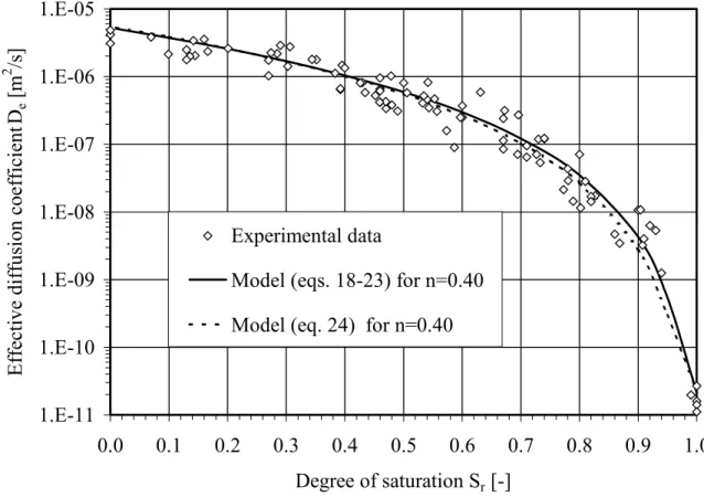
Figure 3 shows a series of test results on non-reactive materials (for Kr = 0), using data taken

from Aubertin et al. (1999, 2000b) and Aachib et al. (2002), with De expressed as a function of

the degree of saturation Sr. Also shown are the curves corresponding to the Collin (1987) model

(equations 18-23) and to equation 24, for a (total) porosity of 0.4 (taken as an average for these test results). As can be seen, both curves provide estimated values that are in relatively good

agreement with the measured values. As mentioned above, such predictive equations provide the starting point in the iterative process to obtain De from testing results.

1.E-11 1.E-10 1.E-09 1.E-08 1.E-07 1.E-06 1.E-05 0.0 0.1 0.2 0.3 0.4 0.5 0.6 0.7 0.8 0.9 1.0 Degree of saturation Sr [-]

Effective diffusion coefficient

De

[m

2 /s]

Experimental data

Model (eqs. 18-23) for n=0.40 Model (eq. 24) for n=0.40

Figure 3. Comparison between diffusion coefficient values measured for different materials (soils, tailings and geosynthetic clay liners – data taken from Aubertin et al. 1999, 2000b, and Aachib et al. 2002) at various Sr, with predicted values obtained with eqs. 18-23 and eq. 24.

For the reaction rate coefficient Kr, Collin (1987, 1998) has proposed a simple model based on

surface kinetic, where the rate varies linearly with the proportion of sulphide minerals (i.e. pyrite). The expression takes into account the total porosity and the grain size through an equivalent grain size diameter DH. This equation can be written as:

[25] _p

H

r K _D6 (1 n)C

where K ′ is the reactivity of pyrite with oxygen ( K ′ ≈ 5x10-10_m3 _O

2/m2pyrite/s or 15.8x10-3m3 O2/m2pyrite/year is used here); Cp is the pyrite content over mass of dry tailings (kg/kg). The

value of DH is estimated here using a relationship with grain size curve parameters, developed for

hydraulic functions (Aubertin et al. 1998; Mbonimpa et al. 2001):

[26] D_H =[1+1.17log(C_U )]D₁₀

where D10 [L] is the diameter corresponding to 10 % passing on the cumulative grain-size

distribution curve and CU [-] is the coefficient of uniformity (CU = D60/D10).

For a typical tailing with D10 = 5x10-6 m, CU = 9 and n = 0.44, the estimated value of Kr is around

1.59x10-7/s (or 0.0137/day, or 5/year) for Cp = 0.1%, 3.97x10-6/s (or 0.343/day, or 125/year)

when Cp = 2.5%, and 1.59x10-5/s (or 1.372/day, or 500/year) for Cp = 10%. Of course, the actual

values of Kr may differ from the estimated ones, as Kr also depends on a number of others factors

including mineralogy and type of sulphides, temperature, oxidation state and bacterial activities (e.g. Hollings et al. 2001).

3.3 Sample results

The application of the proposed interpretation method for the laboratory tests, to determine De

and Kr, is shown in the following using POLLUTE (Rowe et al. 1994). This software has been

employed extensively over the years to analyse tests results and to evaluate the flux corresponding to various cover systems (e.g. Aubertin et al. 1995, 1997c, 1999, 2000a, 2000b; Aachib 1997; Mackay et al. 1998; Yanful et al. 1999). The equations and numerical methods used in POLLUTE have been presented by Rowe and Booker (1985, 1987). This computer program was initially developed for modeling solute transport through saturated porous media. It can be used for gas diffusion in unsaturated media when the equivalent (diffusion) porosity θeq is

In the code, the reaction rate coefficient is defined from a half-time life t1/2* (as an analogy to a

radioactive decay parameter) which, in the case of a first-order reaction, can be expressed as:

[27] r eq * r * 2 / 1 ln_K2 K 2 ln t = =θ

As illustrative examples, typical parametric calculations are performed for anticipated test results. Table 1 gives the characteristics used for 6 cases investigated. For these sample calculations, the heights of the source and receptor reservoirs are fixed at 3 cm, the height of the sand layer is 2 cm, and that of the tested materials (tailings) is 5 cm. Two values for the degree of saturation Sr are considered: 0.90 (cases 1 to 3) and 0.75 (cases 4 to 6). This range of Sr-values

can be observed in practice in the capillary retention layer. The coefficient of diffusion used for modeling is estimated by equations 18 to 23, which give somewhat larger (more conservative) values than eq. 24 (see Fig. 3). For each Sr, three reactivities are considered; tailings are inert (Kr

= 0/s), slightly reactive (Kr = 9.51x10-8/s or 3/year), and strongly reactive (Kr =6.34x10-6/s or

200/year). The properties of the sand used as the underlying coarse material are kept identical for the 6 cases.

Table 1. Material characteristics used for the parametric calculations, to illustrate the test interpretation (Figures 4 and 5).

Material Sr [-] n [-] θa [-] θeq [-] De [m2/s] D* [m2/s] Kr [1/s] Kr* [1/s] Case 0 0 Case 1 Tailings 0.90 0.44 0.044 0.056 4.59x10-9 8.21x10-8 9.51x10-8 1.70x10-6 Case 2 6.34x10-6 1.13x10-4 Case 3 0 0 Case 4 Tailings 0.75 0.44 0.110 0.120 7.71x10-8 6.43x10-7 9.51x10-8 7.93x10-7 Case 5 6.34x10-6 5.29x10-5 Case 6 Sand 0.15 0.40 0.340 0.341 3.12x10-6 9.14x10-6 0 0 All cases

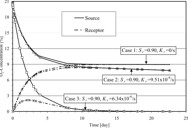
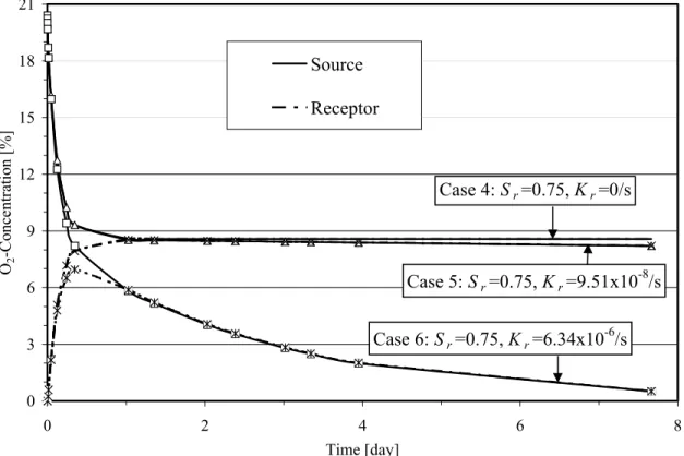
Figures 4 and 5 show the temporal evolution of the oxygen concentration (in %) in the source and receptor reservoirs, as obtained from calculations performed with POLLUTE. The influence of oxygen consumption on the concentration values is particularly well illustrated with these results. For non reactive materials (cases 1 and 4), an equilibrium (no gradient) state is reached after a relatively short time; this time is smaller when Sr is reduced. For slightly reactive materials (cases

2 and 5), a pseudo-steady state is approached, but oxygen consumption decreases the concentration continuously. For a large reactivity (cases 3 and 6), the influence of oxidation is very significant and equilibrium occurs only when all the available oxygen has been consumed.

0 3 6 9 12 15 18 21 0 5 10 15 20 25 Time [day] O2 -Concentration [%] Source Receptor Case 1: Sr=0.90, Kr=0/s Case 2: Sr=0.90, Kr=9.51x10-8/s Case 3: S_r=0.90, K_r=6.34x10-6/s

Figure 4. Temporal evolution of concentration in the source and receptor reservoirs, obtained numerically with POLLUTE, for typical testing conditions (cases 1 to 3 in Table 1).

0 3 6 9 12 15 18 21 0 2 4 6 8 Time [day] O2 -Concentration [%] Source Receptor Case 4: Sr=0.75, Kr=0/s Case 5: Sr=0.75, Kr=9.51x10-8/s Case 6: Sr=0.75, Kr=6.34x10-6/s

Figure 5. Temporal evolution of concentration in the source and receptor reservoirs, obtained numerically with POLLUTE, for typical testing conditions (cases 4 to 6 in Table 1).

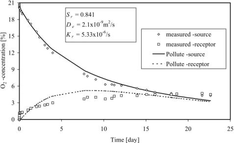
The proposed measuring approach and corresponding interpretation were used to determine the actual oxygen diffusion coefficient De and reaction rate coefficient Kr of two reactive tailings

(from sites SC and LTA located in Québec). The curves with the back calculated values of De

and Kr for which concentration profile approximately match the experimental data are shown in

Figures 6 and 7. In these two cases, the De and Kr values are fairly close to estimated values

obtained from the semi-empirical solutions given above. The results show in particular that the tailings from site LTA are highly reactive (Kr=5.33x10-6/s, or 168 /year). This site has been

covered with a layered system.

The measurement approach presented here for laboratory tests can also be adapted to in situ conditions (e.g. Aubertin et al. 2000a; Mbonimpa et al. 2000), but this aspect is not presented here.

0 3 6 9 12 15 18 21 0 5 10 15 20 25 Time [day] O2 -concentration [%] measured -source measured -receptor Pollute -source Pollute -receptor S_r = 0.841 De = 2.1x10-9m2/s Kr = 5.33x10-6/s

Figure 6. Estimates of De and Kr by comparison of the concentration values evaluated with

POLLUTE and measured in lab tests on SC tailings (height of sample = 47.1 mm, height of source reservoir = 31.9 mm, height of receptor reservoir = 30.8 mm, and n=0.455).

0 3 6 9 12 15 18 21 0 5 10 15 20 25 30 35 40 45 Time [day] O2 -concentration [%] measured -source measured -receptor Pollute -source Pollute -receptor Sr = 0.902 D_e = 3.4x10-10_m2_/s Kr = 5.42x10-7/s

Figure 7. Estimates of De and Kr by comparison of the concentration values evaluated with

POLLUTE and measured in lab tests on LTA tailings (height of sample = 48.2 mm, height of source reservoir = 27.8 mm, height of receptor reservoir = 30.8 mm, and n=0.480).

4. TYPICAL APPLICATIONS

4.1 Reference systems and basic calculations

The analytical equations presented above are now used to estimate the oxygen fluxes at the base and at the surface of a partly saturated, reactive or non-reactive, cover material. To validate the proposed equations, the resulting solutions are first compared to those obtained from numerical calculations. Various cases have been investigated, and some of the most relevant results are presented in the following. More emphasis is placed on the oxygen flux at the base of the cover (eq. 14) than at the cover surface (eq. 17), because the former is more relevant for the evaluation of cover efficiency.

The system being investigated here is a CCBE made of 3 layers: sand/silt/sand (layers C-D-E in Figure 1). It is similar to covers installed at the LTA site (McMullen et al. 1997; Ricard et al. 1997, 1999) and at the Lorraine site (Dagenais et al. 2001). Three cases (A, B and C) have been considered for these oxygen flux calculations. In all cases, an artificial silt (tailing) has been used for the water retention layer (see Table 2). The tailings in the cover for cases A and B are non-reactive (Kr = 0), while those of case C are slightly reactive (but non acid generating). It should

be recalled here that such type of cover has been investigated thoroughly for unsaturated flow and water distribution using instrumented column tests (Aubertin et al. 1995, 1997c; Aachib 1997), inclined layered systems (Aubertin et al. 1997b; Bussière 1999; Bussière et al. 2000), and in situ experimental cells (Aubertin et al. 1997a, 1999). Field work has also been performed on an actual CCBE made with a slightly reactive tailing (Aubertin et al. 2000a).

For the calculations presented below, the values of De were obtained from equations 18-23, for

situations representing worst case scenarios in terms of the degree of saturation (i.e. a long drought period).

Table 2. Material characteristics defined for the three-layer covers investigated (see Figures 8, 9, 10, and 23). Material L (cm) n (-) e (-) γd (g/cm3) Sr (%) θeq (-) De (m2/s) D* (m2/s) eq

θ

Sand 30 0.29 0.41 2.04 13.5 0.2520 2.28E-06 9.05E-06

A Tailings 60 0.46 0.87 1.69 83.1 0.0890 2.42E-08 2.72E-07 0.0914 5.64E-07 0

Sand 40 0.29 0.40 2.05 28.3 0.2104 1.27E-06 6.04E-06

Sand 25 0.33 0.48 2.05 8.9 0.3015 3.10E-06 1.03E-05

B Tailings 30 0.44 0.80 1.56 95.2 0.0338 5.34E-10 1.59E-08 0.0336 5.29E-07 0

Sand 45 0.30 0.42 2.05 24.6 0.2284 1.54E-06 6.75E-06

Sand 30 0.33 0.49 5.0 0.3140 3.56E-06 1.13E-05

C Tailings 80 0.44 0.80 85.0 0.0770 1.61E-08 2.09E-07 0.0783 4.10E-07 3 values1

Sand 50 0.40 0.67 15.0 0.3418 3.12E-06 9.14E-06

1 _{Three different K}

The actual boundary conditions in the field correspond fairly well to those presented above for the analytical solutions (equations 9 and 14). Above the cover and in the top sand layer (which is easily drained), the oxygen concentration C(z=0, t≥0) is C0 = 0.276 kg/m3. Below the cover, it

has been considered that concentration CL (z ≥ L, t>0)=0, which is a conservative (pessimistic)

condition that corresponds to a rapid oxygen consumption by the reactive tailings under the cover. This condition provides the upper bound value of the concentration gradient between the top and bottom part of the cover, and thus the upper bound value of the available oxygen flux (all other factors being equal).

For the situations of interest, POLLUTE does not directly calculate the flux F at the bottom and surface of the cover (or of the water retention layer). It rather provides a concentration profile over time and the total amount Q of the substance diffusing through the cover at a given depth z and time ta (i.e. =

∫

a t 0 dt ) t, z ( F

Q , where ta is the active diffusion period). The flux can

nevertheless be obtained by either differentiation the Q-t relation (δQ/δt) or simply by using equation 1 and the concentration of two adjacent points C(z, and z-δz) at time t (Aubertin et al. 1999; Joanes 1999).

For the sample calculations shown here, it is assumed that material and moisture distribution in each layer are uniform, and that parameters θeq, De and Kr take a constant value for the

calculation period. With POLLUTE, these simplifications are not required as it is possible to work with parameters varying in space (by dividing the layer in sublayers) and over the time (by integrating for different conditions). The examples shown here nevertheless help to illustrate the calculation process, and to validate the analytical solutions.

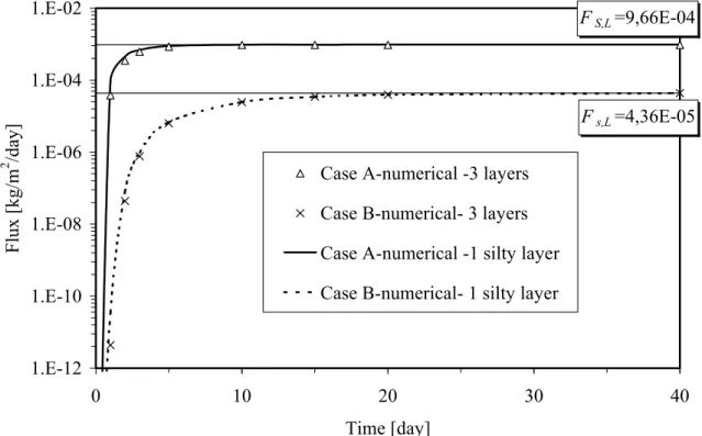
In a 3 layer–system (sand/silt/sand), it has been demonstrated previously that during a drought, the two drained sand layers have the same O2-concentration as the adjacent media because of their high De compared to the silt, hence, C0 =0.276 kg/m3 in the top sand layer and CL=0 in the

bottom sand layer (Aachib et al. 1993). The calculation procedure, with equations 9 and 14, can then be applied to the water retention layer only. It is shown in Figure 8, from calculations made

with POLLUTE, that neglecting the presence of the two sand layers when evaluating the oxygen flux provides essentially the same results as when incorporating them in the calculations. The limitation to this approach is further addressed below.

FS,L=9,66E-04 Fs,L=4,36E-05 1.E-12 1.E-10 1.E-08 1.E-06 1.E-04 1.E-02 0 10 20 30 40 Time [day] Flux [kg/m 2 /day]

Case A-numerical -3 layers Case B-numerical- 3 layers Case A-numerical -1 silty layer Case B-numerical- 1 silty layer

Figure 8. Comparison of temporal evolution of the oxygen bottom flux obtained by numerical solution for the three-layered systems A and B described in Table 2, and for the moisture retention (silty) layer alone; Fs,L is the steady state flux given by eq. 10.

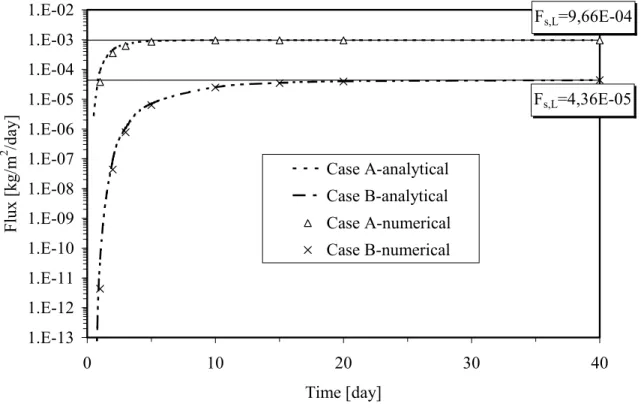
Figure 9 makes a comparison between the flux at the base of the cover (or the water retention layer) obtained from equation 9 and with POLLUTE, for cases A (low saturation) and B (high saturation), with a non reactive material (i.e. water retention layer). The results obtained by both approaches show an excellent agreement. In these two cases, a steady state flux is reached after about 7 days (case A) and 30 days (case B), as was predicted by equation 10. This Figure shows the influence of the cover characteristics on the flux. The total amount Q of oxygen reaching the tailings is provided by the surface below the curve for the given period. Knowing beforehand the

amount of time required to reach steady state, starting with F = 0 after the freezing winter months, is very important to obtain Q for the final design configuration.

F_s,L=9,66E-04 Fs,L=4,36E-05 1.E-13 1.E-12 1.E-11 1.E-10 1.E-09 1.E-08 1.E-07 1.E-06 1.E-05 1.E-04 1.E-03 1.E-02 0 10 20 30 40 Time [day] Flux [kg/m 2 /day] Case A-analytical Case B-analytical Case A-numerical Case B-numerical

Figure 9. Comparison of the temporal evolution of the oxygen bottom flux obtained by analytical and numerical solutions on structure A and B (see Table 2) built with non reactive materials; the analytical solutions are applied to the moisture retention layer alone; Fs,L is the steady state flux

given by eq. 10

When the silt (water retaining) layer contains some small amount of reactive minerals (i.e. sulphides in tailings), it consumes part of the oxygen that diffuses through it. As stated above, this can be helpful in reducing the amount of O2 that reaches the reactive tailings underneath. Figure 10 shows a comparison between the proposed analytical solution (equation 14) for system C (Table 2) and the solution obtained from POLLUTE. Three values of the reaction rate parameter Kr have been considered: Kr = 3.17x10-8, 1.59x10-7, and 4.76x10-7 per second (or 1, 5,

also presented in the Figure to illustrate the effect of cover material reactivity on the flux. From Figure 10, it can be concluded that the analytical solution is in excellent agreement with the numerical solution. It also shows that increasing Kr of the cover material can significantly reduce

the amount of oxygen reaching the reactive material.

0.E+00 1.E-04 2.E-04 3.E-04 4.E-04 5.E-04 0 10 20 30 40 Time [day] Flux [kg/m 2 /day] Steady state(non-reactive) Analytical solution Analytical solution Analytical solution Analytical solution Numerical solution Numerical solution Numerica solution Numerical solution K_r = 0/s Kr = 3.17x10-8/s K_r = 1.59x10-7/s K_r = 4.76x10-7/s

Figure 10. Temporal evolution of the oxygen flux at the base obtained by analytical and numerical solutions, in the case of a reactive moisture retention material layer for various Kr

values (system C in Table 2); the analytical solutions are applied to the moisture retention layer alone.

Relatively to the temporal evolution of the surface flux entering the cover, analytical results obtained with equation 17 have also been validated with POLLUTE (results not shown here). Such surface fluxes and those reaching the base of the cover are shown in Figure 11, in the case of a water retention material layer with a thickness of 0.8 m, a porosity of 0.44, a degree of saturation of 0.85, and a diffusion coefficient estimated with equations 18–23.

F_ss=9.71E-04 Fss=2.72E-04 F_ss=2.08E-03 F_ss=5.36E-05 F_s,L=4.79E-04 1.E-08 1.E-07 1.E-06 1.E-05 1.E-04 1.E-03 1.E-02 1.E-01 1.E+00 0.1 1 10 100 Time (day) Flux (kg/m 2 /day) n = 0.44 Sr= 0.85 s-surface b-base 1-K_r=0/s 2-Kr=9.51x10-8/s 3-Kr=4.76x10-7/s s1 s2 s3 b1 b2 b3

Figure 11. Temporal evolution of the base and surface fluxes obtained from analytical solutions (eqs. 14 and 16 respectively) in the case of a reactive material layer with a porosity of 0.44 and a degree of saturation of 0.85 (the diffusion coefficient is estimated with relations 18 –23), with three different reaction rate coefficients; Fs,L and Fss are the steady state fluxes (calculated with

eqs. 15 and 17 respectively).

The influence of oxygen consumption is also seen from Figure 11, where three different reaction rate coefficients Kr (0, 9.51x10-8, and 4.76x10-7/s or 0, 3, and 15/year) have been considered. The

surface flux entering the cover decreases over time while the flux reaching the base of the cover increases. These fluxes eventually reach a steady state (when the boundary conditions don’t change). For reactive materials, the base and surface steady state fluxes given by equations 15 and 17 are different. The smaller the value of Kr, the smaller is the difference between the two

steady state fluxes. This difference corresponds to the amount of oxygen being consumed by the cover material. In the case of a non-reactive material (Kr=0/s), the steady state flux established is

obtained with equation 10; it is the same for surface and base fluxes (see curves s1 and b1 in Figure 11).