Approximate Policy Iteration for Closed-Loop
Learning of Visual Tasks
S´ebastien Jodogne, Cyril Briquet, and Justus H. Piater
University of Li`ege — Montefiore Institute (B28) B-4000 Li`ege, Belgium
{S.Jodogne,C.Briquet,Justus.Piater}@ULg.ac.be
Abstract. Approximate Policy Iteration (API) is a reinforcement learn-ing paradigm that is able to solve high-dimensional, continuous control problems. We propose to exploit API for the closed-loop learning of map-pings from images to actions. This approach requires a family of function approximators that maps visual percepts to a real-valued function. For this purpose, we use Regression Extra-Trees, a fast, yet accurate and versatile machine learning algorithm. The inputs of the Extra-Trees con-sist of a set of visual features that digest the informative patterns in the visual signal. We also show how to parallelize the Extra-Tree learn-ing process to further reduce the computational expense, which is often essential in visual tasks. Experimental results on real-world images are given that indicate that the combination of API with Extra-Trees is a promising framework for the interactive learning of visual tasks.
1
Introduction
Since the rise of embedded CCD sensors, many robots are nowadays equipped with cameras and, as such, face input spaces that are extremely high-dimensional and potentially very noisy. Therefore, though real-world visual tasks can often be solved by directly connecting the visual space to the action space (i.e. by learning a direct image-to-action mapping), such mappings are especially hard to derive by hand and should be learned by the robotic agent. The latter class of problems is commonly referred to as Vision-for-Action. A breakthrough in modern AI would be to design an artificial system that would acquire object or scene recognition skills using only its interactions with the environment.
In this paper, an algorithm is introduced for closed-loop learning of image-to-action mappings. Our algorithm is defined within the biologically-inspired framework of reinforcement learning (RL) [1]. RL models an agent that learns a percept-to-action mapping through its interactions with the environment: It is only implicitly guided through a reinforcement signal , which is generally delayed. RL is an attractive framework for Vision-for-Action problems. Unfortunately, basic RL algorithms are highly sensitive to the noise and to the dimensionality of the percepts, which forbids their direct use when solving visual tasks. We have previously proposed an algorithm that adaptively discretizes the visual space into a small number of visual classes [2]. Schematically, a decision tree is
progressively built that tests, at each of its nodes, the presence of one highly informative image pattern (a visual feature). The tree is incrementally refined in a sequence of attempts to remove perceptual aliasing. This dramatically reduces the size of the input space, so that standard RL algorithms become usable.
One might wonder, however, whether the feature selection process is actually desirable, as it might introduce a high variance in the computed image classi-fiers, just as in the case of incremental learning of decision trees [3]. Furthermore, selecting visual features requires the introduction of an equivalence relation be-tween the features. This relation is difficult to define. Often, a fixed threshold on a metric in feature space is used. However, modifying this threshold can lead to significant changes in the learned image-to-action mapping.
We describe a method that uses the whole set of visual features, without taking decisions involving a subset of informative features, and without relying on a similarity measure between them. In other words, we exploit the raw visual features. As visual data can be sampled only sparsely, we resort to the embedding of function approximators inside the RL process. Among the RL algorithms that use function approximators, we use Approximate Policy Iteration (API) [1]. API together with a linear approximation architecture has already been proposed in the context of continuous state spaces, giving rise to the Least-Squares Policy Iteration algorithm [4].
The Visual Approximate Policy Iteration (V-API) is defined, which is an in-stance of API designed to work in visual spaces. V-API uses Regression Extra-Trees, a family of nonparametric function approximators. This choice is moti-vated by the low bias and variance, as well as the good performance in generaliza-tion of the Extra-Trees [3]. Furthermore, Classificageneraliza-tion Extra-Trees are successful for solving image classification tasks [5]. To the best of our knowledge, this makes of V-API the first application of API to high-dimensional discrete spaces. Thus, V-API is potentially of major interest, as it proves that fully automatic, non-parametric RL methods can succeed in visual tasks. Likewise, the embedding of Extra-Trees in API is novel, and should also be useful in continuous state spaces. Even if the computational expense of Extra-Trees is small with respect to other machine learning algorithms, the complexity of visual spaces still prevents their direct use in V-API. An additional contribution is to parallelize the Extra-Trees learning algorithm, which greatly reduces the execution time of V-API.
The paper is organized as follows. Firstly, we discuss the three important tools that are used inside V-API, namely the Modified Policy Iteration algorithm, the extraction of visual features and the Regression Extra-Trees. Then, we formally describe V-API and the distributed learning of Extra-Trees. Finally, we conclude with experimental results on a complex, visual navigation task.
2
Theoretical Background
2.1 Modified Policy Iteration
V-API is defined in the framework of Reinforcement Learning (RL). In RL, the environment is traditionally modeled as a Markov Decision Process (MDP). An
MDP is a quadruple hS, A, T , Ri, where S is a finite set of states or percepts1,
A is a finite set of actions, T is a probabilistic transition function from S × A to S, and R is a reinforcement signal from S × A to R. An MDP obeys the following discrete-time dynamics: If at time t, the agent takes the action at while the environment lies in a state st, the agent perceives a numerical
reinforcement rt+1 = R(st, at), then reaches some state st+1 with probability
T (st, at, st+1). Therefore, from the point of view of the agent, an interaction
with the environment is summarized as a quadruple hst, at, rt+1, st+1i.
A (deterministic) percept-to-action mapping (or, equivalently, a control pol-icy) is a fixed function π : S 7→ A from percepts to actions. Each control policy π is associated with a state-action value function Qπ(s, a) that gives, for each state s ∈ S and each action a ∈ A, the expected discounted return obtained by starting from state s, taking action a, and thereafter following π:
Qπ(s, a) = Eπ (∞ X t=0 γtrt+1| s0= s, a0= a ) , (1)
where γ ∈ [0, 1[ is the discount factor that gives the current value of the future reinforcements, and where Eπ denotes the expected value if the agent follows
the mapping π. Theory shows that all the optimal policies for a given MDP share the same Q function, denoted Q∗and called the optimal state-action value function, that always exists. Once the optimal state-action value function Q∗ is known, an optimal percept-to-action mapping π∗ is easily derived by choosing:
π∗(s) = argmax
a∈A
Q∗(s, a), for each s ∈ S. (2) Dynamic Programming (DP) is a set of algorithmic methods for solving MDPs. DP algorithms assume the knowledge of the transition function T and of the reinforcement signal R. The well-known Modified Policy Iteration (MPI) [6] is an important DP algorithm that will be useful in the sequel. Starting with an initial, arbitrary percept-to-action mapping π0, MPI builds a sequence of
increasingly better policies π1, π2, . . . by relying on two interleaved learning
pro-cesses: (1) policy estimation (the critic component), which computes the Qπk
state-action value function of the current policy πk; and (2) policy improvement
(the actor component), which uses Qπk to generate an improved policy π
k+1.
The algorithm stops when there is no change between successive policies. Here is a brief description of the two processes:
Policy estimation: Qπk is computed by building a sequence of state-action
value functions Q0, Q1, . . . until convergence using the update rule:
Qi+1(s, a) = R(s, a) + γ
X
s0∈S
T (s, a, s0)Qi(s0, π(s0)). (3)
After convergence, Bellman’s theorem [1] shows that Qik = Q
πk. Q
0 can be
chosen freely (generally, Q0(s, a) = 0 for each s ∈ S and a ∈ A).
1
MDP assumes the full observability of the environment, which allows us to talk indifferently about states and percepts. In visual tasks, S is a set of images.
Policy improvement: At each state s ∈ S, πk(s) is replaced by the action with
the best state-action value (as computed by the policy estimation process): πk+1(s) = argmax
a∈A
Qπk(s, a). (4)
Finally, reinforcement learning is defined as the counterpart of DP when the transition function T and the reinforcement signal R are unknown. The input of RL algorithms is basically a database of interactions hst, at, rt+1, st+1i.
2.2 Extraction of Visual Features
Because standard RL algorithms rely on a tabular representation of the value functions, they quickly become impractical as the number of possible percepts increases. This is evidently a problem in visual tasks, as images are high-dimen-sional and noisy. Similar problems often arise in many fields of Computer Vision. For this purpose, the popular, highly successful local-appearance methods have been introduced [7, 8]. They postulate that, to take the right decision in a visual problem, it is often sufficient to focus one’s attention only on a few interesting patterns occurring in the images. They summarize the images as a set of visual features, that are vectors of real numbers. Formally, they introduce a feature transform F : S 7→ P(Rn), where S is the set of images and P denotes the power set. For an image s ∈ S, F (s) typically contains between 10 and 1000 visual features. Most feature transforms have in common that (1) they select in-terest points in the image (e.g. by detecting discontinuities in the visual signal), and (2) they compute a local description of the neighborhood of the interest points. As an illustration, here are two possible choices of feature transforms:
1. “Traditional” feature transforms, that use a standard interest point detector (Harris, Harris-affine, Hessian-Laplace,. . . ) [7] in conjunction with a stan-dard local descriptor (steerable filters, local jet, SIFT,. . . ) [8].
2. Randomized feature transforms. They randomly select a fixed number of subwindows in the image (a subwindow is a rectangle that has an arbitrary position, scale and orientation). Then, the subwindows are downscaled to a patch of fixed size (typically 11 × 11), in a fixed colorspace (graylevel, RGB or HSV). This simple approach is very fast, as well as highly successful [5]. V-API uses such methods to digest an image into a set of raw visual features.
2.3 Regression Extra-Trees
As discussed in the Introduction, V-API rely on Extra-Trees [3]. We restrict our study of Extra-Trees to the case where all attributes (both the inputs and the output) are numerical. An Extra-Tree model is constituted by a forest of M independent decision trees. Each of their internal nodes is labeled by a threshold on one of the input attributes, that is to be tested in that node. The leaves are labeled by a regression output. The regression response for a sample is ob-tained by computing the response of each subtree. This is achieved by starting
at the root node, then progressing down the tree according to the result of the thresholding tests found during the descent, until a leaf is reached. By doing so, each subtree votes for a regression output. Finally, the mean of these outputs is assigned to the sample.
The subtrees are built in a top-down fashion, by successively splitting the leaf nodes where the output variable varies. For each input variable, the algorithm computes its variation bounds and uniformly chooses one random threshold be-tween those bounds. Once a threshold has been chosen for every input variable, the split that gives the best score on the regression output is kept. The tree con-struction is stopped when the output is constant in the leaf. This will guarantee that learning bias is small, as well as learning variance thanks to the aggregation of a sufficient number of randomized trees.
Algorithms 1 and 2 describe how to build an Extra-Tree model. In this pseudo-code, xi ∈ Rn contains the input attributes of the ith sample in the
learning set and yi ∈ R is the observed regression output for this sample. We
assume the existence of a function score({hxi, yii}, v, t) that returns the score
of the threshold t on the variable v in the database {hxi, yii}. In our
implemen-tation, variance reduction was used as the score function. These algorithms are identical to those presented by Geurts et al. [3] and are restated here to com-plement the description of our distributed algorithms (cf. Section 3.5). We refer the reader to Geurts et al. [3] for a complete and thorough treatment.
3
Visual Approximate Policy Iteration
3.1 Nonparametric Approximate Policy Iteration
In the next sections, a general, nonparametric RL version of Approximate Policy Iteration (API) is described. Nonparametric API is a generalization of MPI that can use any kind of nonparametric function approximators. This is in contrast to Least-Squares Policy Iteration [4] that explicitly targets continuous state spaces and uses linear approximation. The two components of MPI (policy estimation and improvement) are adapted so as to compute the state-action value function of a policy without relying on any knowledge of the underlying MDP.
The existence of an oracle called learn is assumed, as we are concerned with nonparametric function approximators. Given a database of samples hst, at, vti,
where stis a state, atis an action and vtis a real number, learn builds a function
approximator that represents a state-action value function Q : S ×A 7→ R that is the closest possible to the given sample distribution. For instance, Algorithm 1 constitutes one possible oracle that is suitable for problems with continuous state space. An oracle for visual spaces will be introduced in Section 3.4.
3.2 Representation of the Generated Policies
Nonparametric API relies on the state-of-the-art principle that was proposed in Least-Squares Policy Iteration [4]: Any state-action value function Q(s, a)
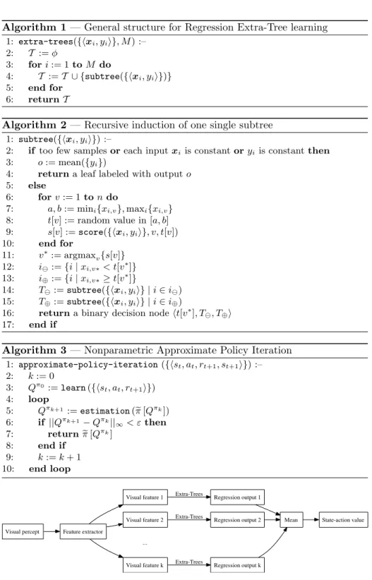
Algorithm 1 — General structure for Regression Extra-Tree learning 1: extra-trees({hxi, yii}, M ) :– 2: T := φ 3: for i := 1 to M do 4: T := T ∪ {subtree({hxi, yii})} 5: end for 6: return T
Algorithm 2 — Recursive induction of one single subtree
1: subtree({hxi, yii}) :–
2: if too few samples or each input xiis constant or yiis constant then
3: o := mean({yi})
4: return a leaf labeled with output o 5: else
6: for v := 1 to n do
7: a, b := mini{xi,v}, maxi{xi,v}
8: t[v] := random value in [a, b] 9: s[v] := score({hxi, yii}, v, t[v]) 10: end for 11: v∗:= argmaxv{s[v]} 12: i := {i | xi,v∗< t[v∗]} 13: i⊕:= {i | xi,v∗≥ t[v∗]} 14: T := subtree({hxi, yii} | i ∈ i ) 15: T⊕:= subtree({hxi, yii} | i ∈ i⊕)
16: return a binary decision node ht[v∗], T , T⊕i
17: end if
Algorithm 3 — Nonparametric Approximate Policy Iteration
1: approximate-policy-iteration ({hst, at, rt+1, st+1i}) :– 2: k := 0 3: Qπ0:= learn ({hs t, at, rt+1i}) 4: loop 5: Qπk+1:= estimation ( e π [Qπk]) 6: if ||Qπk+1− Qπk||∞< ε then 7: returneπ [Qπk] 8: end if 9: k := k + 1 10: end loop
Visual percept Feature extractor
Visual feature 1 Visual feature 2 ... Visual feature k Regression output 1 Extra-Trees Regression output 2 Extra-Trees Regression output k Extra-Trees
Mean State-action value
induces a greedy policy eπ [Q] that always selects the action maximizing Q:
e
π [Q] (s) = argmax
a∈A
Q(s, a), for each s ∈ S.2 (5)
This property enables us to deal only with state-action value functions, and never directly with policies. So, there is no need of a separate representation system for policies. In terms of the notation of Section 2.1, nonparametric API does not keep track of πk = eπ [Q
πk−1], but only of Qπk. The policy π
k is evaluated on
demand from Qπk−1 through Equation 5. Thanks to this implicit representation
of the policies, the policy improvement step becomes trivial: It is sufficient to define Qπk+1as the state-action value function of the greedy policy with respect
to Qπk, that is computed by the policy estimation component.
Algorithm 3 summarizes the backbone of nonparametric API. The input of the algorithm is a database of interactions hst, at, rt+1, st+1i, which makes of
nonparametric API an off-policy, model-free RL algorithm. The third line builds an initial policy π0 that maximizes immediate reinforcements. The algorithm
stops when the difference between two successive Qπk drops below a threshold.
3.3 Nonparametric Approximate Policy Estimation
The estimation component in Algorithm 3 computes the state-action value function Qπk+1 of a policy
e
π [Qπk] given the input database of interactions
hst, at, rt+1, st+1i. To this end, a sequence of state-action value functions Qi(s, a)
is generated. This is done according to the principle of Modified Policy Iteration, but the functions Qi are now function approximators that are built through the
learn oracle. As the underlying MDP is unknown, the update rule of Equation 3 cannot be used. Instead, we use the stochastic version of this equation:
Qi+1(s, a) = R(s, a) + γ Qi(δ(s, a),π [Qe πk] (δ(s, a))) . (6)
Hence, the update rule that is induced by the database of interactions is: Qi+1:= learn ({hst, at, rt+1+ γ Qi(st+1,eπ [Qπk] (st+1))i}) . (7)
A new Extra-tree model is learned through each application of this update rule. This learning process stops when the difference between two successive Qidrops
below a threshold. Q0can be chosen freely. In practice, Q0is set to Qπk. This is
a starting point that reduces the number of iterations before convergence, as the policyπ [Qe πk+1] generally shares common decisions with
e
π [Qπk]. This algorithm
can be motivated similarly than Fitted Q Iteration [9]: The stochastic aspect of the environment will eventually be captured by the function approximators.
3.4 Visual State-Action Value Function Approximators
So far, we have not defined a family of function approximators that is suitable for visual tasks. As motivated in the Introduction, we propose to take advantage
2
of the raw visual features. Therefore, Regression Extra-Trees cannot be used directly, for two reasons: (1) The action input is discrete, and cannot be fed into a Regression Extra-Tree model as defined in Section 2.3; and (2) feature transforms map one visual percept to many visual features (cf. Section 2.2).
The solution to the first problem is straightforward: The single Extra-Tree model Q(s, a) is replaced by |A| Extra-Tree models Qa(s), one for each possible
action a ∈ A. The latter problem is more fundamental, and is solved by applying the Extra-Trees model independently on each visual feature in the input image. This process generates one regression output per visual feature. Then the value of the function approximator is defined as the mean of these regression out-puts. This approach is depicted in Figure 1, and is directly inspired by recent, successful results about image classification through Extra-Trees [5].
The learn oracle for this type of function approximators is now defined formally. Given a database of samples hst, at, vti (where st are images), the
Extra-Trees model Qa that corresponds to the action a ∈ A is defined as:
Qa(s) := extra-trees ({hxi, yii | (∃t ∈ Ta)(xi∈ F (st) ∧ yi= vt)}; M ) , (8)
where F is the used feature transform, and Ta = {t | at= a} is the set of time
stamps for the interactions that are labeled with the action a. Intuitively, for each sample hst, at, vti, all the visual features in the image stare associated with
the value vtin the database that is used to train the Extra-Tree model Qat.
Nonparametric API along with such a family of function approximators will be referred to as the Visual Approximate Policy Iteration (V-API) algorithm.
3.5 Parallelizing Extra-Trees
V-API applies Regression Extra-Trees on large databases. This induces a high computational cost for the learning of Extra-Trees. We propose to reduce this computational expense by taking advantage of the extremely parallelizable na-ture of Algorithm 1: Each execution of Algorithm 2 is totally independent of other instances of the same algorithm, and each subtree can be computed in a separate computational task. In other words, the learning of Extra-Tree models can be formulated as a so-called bag of tasks, where tasks are independent and can be processed on separate computer nodes. Once all the tasks are completed, it is straightforward to merge all the subtrees to generate the Extra-Tree model. Our implementation of Regression Extra-Trees follows this principle. The resulting speedup is huge: If N homogeneous hosts are used, the computation time roughly equals dM/N eT + U , where M is the parameter of Algorithm 1, T is the mean amount of time for building one single subtree, and U corresponds to the distribution time of the database among all the hosts.
Note that if no attention is paid, the transmission overhead U can quickly become a bottleneck. Indeed, the same large database has to be sent to N hosts by the central task manager, which causes both reduction of bandwidth and augmentation of network congestion effects. One possible solution is to rely on the use of UDP multicast. Unfortunately, due to the lack of flow control in UDP, slow hosts will be overwhelmed by the massive amount of data they receive.
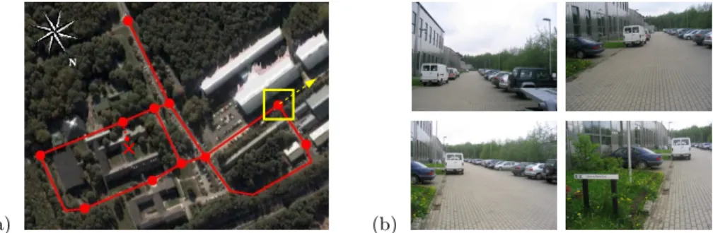
(a)
N
(b)
Fig. 2. (a) Navigation around Montefiore Institute. Red spots corresponds to the places between which the agent moves. The agent can only follow the links between the different spots. On this map, Montefiore Institute is labeled by a red cross. (b) The percepts of the agent. Four different percepts are shown that correspond to the location and viewing direction marked in yellow on the map on the left.
We have therefore used the peer-to-peer BitTorrent protocol [10] to distribute the databases. Schematically, in BitTorrent, each host becomes part of a swarm that grabs all the pieces of a file. Whenever a host acquires a piece, this piece is made available for download to the other hosts. A distinguished host, the tracker , is used to keep track of the hosts that belong to the swarm. This approach for file distribution is elegant and scalable, and indeed highly reduces the transmission overhead U , making it roughly independent of the number of hosts in the cluster. Our solution should be useful in many other distributed computing applications, and especially in the context of distributed data mining and Grid computing.
4
Experimental Results
We have applied the V-API to a simulated navigation task. In this task, the agent moves between 11 distinct locations of our campus (cf. Figure 2 (a)). Every time the agent is at one of the 11 locations, its body can aim at 4 possible orientations: North, South, West, East. It can take 3 different actions: Turn left, turn right, go forward. Its goal is to enter the Montefiore Institute, where it gets a reward of 100. Turning left or right induces a penalty of −5, and moving forward, a penalty of −10. The discount factor γ was set to 0.8.
The agent does not have access to its position and its orientation. Rather, it only perceives a picture of the area that is in front of it. So, the agent has to connect images directly to the appropriate reactions without knowing the under-lying physical structure of the task. For each possible location and each possible viewing direction, a database of 24 images of size 1024 × 768 with viewpoint changes was collected. Those 44 databases were divided into a learning set of 18 images and a test set of 6 images (cf. Figure 2 (b)). V-API has been applied on a static database of 10,000 interactions that has been collected using a fully randomized exploration policy. The same database is used throughout the entire V-API algorithm, and only contains images that belong to the learning set.
In our experiments, we have used traditional feature transforms with the SIFT descriptors (whose dimension is n = 128) [11]. This choice is mostly arbi-trary. Randomized feature transforms are promising, and will be investigated in future work. The parallel implementation of Regression Extra-Trees runs on a testbed cluster of N = 67 heterogeneous ix86 machines. It consists of a set of 27 AMD Athlon 1800+, 27 Intel Celeron 2.4Ghz, and 13 Intel Pentium IV 2.8Ghz CPUs. They are interconnected via a switched 100Mbps Ethernet network.
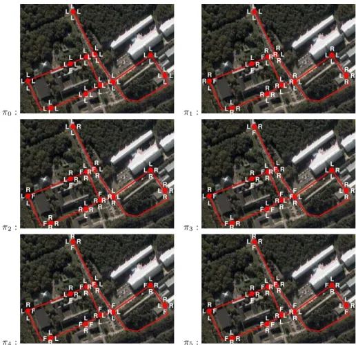
Figure 3 shows the sequence of policies that is generated by V-API. The algorithm stops after 6 iterations, which is a surprisingly small number. A total of 147 Extra-Tree models were generated that correspond to 49 = 147/|A| visual state-action value functions (as defined in Section 3.4). The overall running time was about 98 hours. This shows the interest of taking advantage of the intrinsic parallelism of Extra-Trees, as this has divided the running time by about fifty. Statistics about the generated policies are given in Figure 4. The error of the last policy in the generated sequence was 1.6% on the learning set and 6.6% on the test set, with respect to the optimal policy when the agent has direct access to its position and viewing direction. These error rates are better than those obtained through RLVC (2% on the learning and 14% on the test set) [12].
The advantage of using BitTorrent is clear: In optimal conditions, if m Extra-Tree models (as discussed above, m = 147) are to be built from databases of typical size S = 80MB, the transmission overhead corresponding to FTP would roughly equal U ≈ m × N × S[MB]/100[Mbps] = 17 hours. Using BitTorrent, this time is approximately reduced to U ≈ m × S[MB]/100[Mbps] = 16 minutes.
5
Conclusions
We have introduced the Visual Approximate Policy Iteration (V-API) algorithm. V-API is designed for the closed-loop solution of visual control problems. It ex-tensively relies on the use of Regression Extra-Trees as function approximators. The embedding of Extra-Trees inside the framework of API is a first important contribution of this paper. Experiments indicate that the algorithm is sound and applicable to non-trivial visual tasks. V-API outperforms RLVC in terms of performance in generalization over the test set. Future work will demonstrate that the proposed combination of nonparametric API with Extra-Trees is a con-venient choice for RL in high-dimensional, continuous state spaces.
We have also shown how to take advantage of the highly parallelizable nature of the induction of Extra-Trees by distributing the construction of the subtrees over a cluster of computers. This allows us to greatly reduce the computational time, which is often an important issue with visual spaces. Of course, other fields of application of Extra-Trees, such as supervised learning [3], image classifica-tion [5] and the Fitted Q Iteraclassifica-tion algorithm [9], will directly benefit from this new economical advantage. Finally, the peer-to-peer BitTorrent protocol was shown to be an effective tool for reducing the database distribution expense.
Unfortunately, even when taking advantage of a cluster of computers, the running time of the algorithm is still relatively long. A compromise seems to
π0: L L L L L L L L L L LL L F L L L LL L L L L L L LL LL L L L L L L L L L L L L L L L π1: L L L L L L F L L L L L L L L L L L L L L L R R F R R R F R R R R R R R RR R R R R R R π2: L L L F L L L L L L L R F RFR R R R R R R R R R R R F L R R L R L F R R L R L R R R F π 3: L L L F L L L L L R F RF RR R R R R R R R F L R R L L F R R L R F L R L F F F L F F L π4: L F L L L L R F RFRR R R R R R F L R R L L F L R F L L F F F L F R L R L L R F R F L π5: L F L L L L R F RF RR R R R R F L R R L L F R L R F L L F F F L F R R L R F F R R R L
Fig. 3. The sequence of policies πkgenerated by V-API. At each location, 4 letters from
the set {F, L, R} are written, one for each viewing direction. Each letter represents the action (go Forward, turn Left, turn Right) that receives the majority of votes in the learning set, for the corresponding pair location / viewing direction.
0 0.05 0.1 0.15 0.2 0.25 0.3 0.35 0.4 0.45 0.5 0 1 2 3 4 5 0 0.05 0.1 0.15 0.2 0.25 0.3 0.35 0.4 0.45 0.5 Learning set Test set
Fig. 4. Policy error as a function of the step counter k. The solid (resp. dashed) plot corresponds to the error rate of the policy πk on the learning (resp. test) set.
exist between the requirement of an equivalence relation among visual features, as in the algorithm RLVC [2], and the use of raw visual features, as in V-API. RLVC runs faster, does not require a cluster of computers, and can be used to generate higher-level visual features [13]. On the other hand, V-API benefits from the full discriminative power of the visual features, exhibits the low variance and bias of Extra-Trees, and requires less parameter tuning. Therefore, V-API and RLVC constitute two complementary techniques. An interesting open question is whether the advantages of these two techniques can be combined.
Acknowledgments. We kindly acknowledge P. Geurts and the pepite s.a. team (http://www.pepite.be/) for providing us with an implementation of the Extra-Trees, which has inspired our parallel implementation. We also wish to thank Prof. L. We-henkel for helpful comments on a preliminary version of this paper, and S. Martin for his valuable help regarding network programming and BitTorrent’s protocol.
References
1. Bertsekas, D., Tsitsiklis, J.: Neuro-Dynamic Programming. Athena Scientific (1996)
2. Jodogne, S., Piater, J.: Interactive learning of mappings from visual percepts to actions. In De Raedt, L., Wrobel, S., eds.: Proc. of the 22nd International Conference on Machine Learning (ICML), Bonn (Germany), ACM (2005) 393–400 3. Geurts, P., Ernst, D., Wehenkel, L.: Extremely randomized trees. Machine
Learn-ing 36(1) (2006) 3–42
4. Lagoudakis, M., Parr, R.: Least-squares policy iteration. Journal of Machine Learning Research 4 (2003) 1107–1149
5. Mar´ee, R., Geurts, P., Piater, J., Wehenkel, L.: Random subwindows for robust image classification. In: IEEE Conference on Computer Vision and Pattern Recog-nition. Volume 1., San Diego (CA, USA) (2005) 34–40
6. Puterman, M., Shin, M.: Modified policy iteration algorithms for discounted Markov decision problems. Management Science 24 (1978) 1127–1137
7. Schmid, C., Mohr, R., Bauckhage, C.: Evaluation of interest point detectors. In-ternational Journal of Computer Vision 37(2) (2000) 151–172
8. Mikolajczyk, K., Schmid, C.: A performance evaluation of local descriptors. In: Proc. of the IEEE Conference on Computer Vision and Pattern Recognition. Vol-ume 2., Madison (WI, USA) (2003) 257–263
9. Ernst, D., Geurts, P., Wehenkel, L.: Tree-based batch mode reinforcement learning. Journal of Machine Learning Research 6 (2005) 503–556
10. Cohen, B.: Incentives build robustness in BitTorrent. In: Proc. of the Workshop on Economics of Peer-to-Peer Systems. (2003)
11. Lowe, D.: Distinctive image features from scale-invariant keypoints. International Journal of Computer Vision 60(2) (2004) 91–110
12. Jodogne, S., Piater, J.: Learning, then compacting visual policies (extended ab-stract). In: Proc. of the 7th European Workshop on Reinforcement Learning (EWRL), Napoli (Italy)(2005) 8–10
13. Jodogne, S., Scalzo, F., Piater, J.: Task-driven learning of spatial combinations of visual features. In: Proc. of the IEEE Workshop on Learning in Computer Vision and Pattern Recognition, San Diego (CA, USA), IEEE (2005)