Closed-Loop Learning of
Visual Control Policies
Ann´ee acad´emique 2006 - 2007
Th`ese de doctorat pr´esent´ee par S´ebastien Jodogne
en vue de l’obtention du grade de Docteur en Sciences (orientation Informatique)
In this dissertation, I introduce a general, flexible framework for learning direct mappings from images to actions in an agent that interacts with its surrounding environment. This work is motivated by the paradigm of purposive vision. The original contributions consist in the design of reinforcement learning algorithms that are applicable to visual spaces. Inspired by the paradigm of local-appearance vision, these algorithms exploit specialized visual features that can be detected in the visual signal.
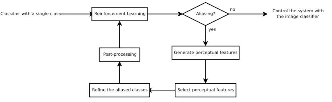
Two different ways to use the visual features are described. Firstly, I introduce adaptive-resolution methods for discretizing the visual space into a manageable num-ber of perceptual classes. To this end, a percept classifier that tests the presence or absence of few highly informative visual features is incrementally refined. New discriminant visual features are selected in a sequence of attempts to remove percep-tual aliasing. Any standard reinforcement learning algorithm can then be used to extract an optimal visual control policy. The resulting algorithm is called Reinforce-ment Learning of Visual Classes. Secondly, I propose to exploit the raw content of the visual features, without ever considering an equivalence relation on the visual feature space. Technically, feature regression models that associate visual features with a real-valued utility are introduced within the Approximate Policy Iteration architecture. This is done by means of a general, abstract version of Approximate Policy Iteration. This results in the Visual Approximate Policy Iteration algorithm. Another major contribution of this dissertation is the design of adaptive-resolu-tion techniques that can be applied to complex, high-dimensional and/or continuous action spaces, simultaneously to visual spaces. The Reinforcement Learning of Joint Classes algorithm produces a non-uniform discretization of the joint space of per-cepts and actions. This is a brand new, general approach to adaptive-resolution methods in reinforcement learning that can deal with arbitrary, hybrid state-action spaces.
Throughout this dissertation, emphasis is also put on the design of general al-gorithms that can be used in non-visual (e.g. continuous) perceptual spaces. The applicability of the proposed algorithms is demonstrated by solving several visual navigation tasks.
Tout d’abord, je souhaite exprimer toute ma gratitude envers Monsieur J. Piater, promoteur de cette th`ese, qui m’a accueilli et m’a propos´e un sujet riche et pas-sionnant. Je lui suis notamment extrˆemement reconnaissant pour toute la confiance qu’il m’a t´emoign´ee en me donnant une grande libert´e dans mes recherches. Qu’il soit aussi remerci´e pour sa gentillesse, pour ses id´ees pr´ecieuses, pour son respect et bien sˆur pour l’encadrement scientifique apport´e au cours de ces trois ann´ees.
Je remercie Messieurs V. Charvillat, R. Munos, L. Paletta, J. Verly et L. Wehenkel, membres du jury, pour avoir accept´e de consacrer du temps `a la lecture et `a l’´evaluation de ce document.
Je suis ´egalement extrˆemement reconnaissant envers le FNRS et Monsieur P.-A. de Marneffe pour m’avoir fourni le support financier n´ecessaire `a la r´ealisation de mon doctorat.
Un de mes plus proches amis m´erite une place toute particuli`ere dans ces remer-ciements. Il s’agit de Cyril Briquet. Qu’il soit bien sˆur remerci´e pour tout le temps pass´e `a la relecture de cette th`ese, pour tous les pr´ecieux conseils prodigu´es et pour notre publication commune. Mais en outre, je lui serai toujours reconnaissant pour le coaching psychologique diablement efficace dont j’ai pu b´en´eficier. Merci aussi `a Elisabeth Spilman pour sa relecture de l’introduction, ce qui lui a donn´e plus de consonances anglophones.
Je tiens ´egalement `a remercier l’ensemble du personnel acad´emique, scientifique, technique et ouvrier de Montefiore qui m’a permis de construire mon doctorat dans une ambiance conviviale et agr´eable. Je ne connais pas la moiti´e d’entre vous `a moiti´e autant que je le voudrais. Mes plus vifs remerciements vont notamment `
a Olivier Barnich, Axel Bodart, Danielle Borsu, Christophe Burnotte, Re-naud Dardenne, Fabien Defays, G´erard Dethier, Damien Ernst, Jean-Marc Franc¸ois, Simon Franc¸ois, Christophe Germay, Pierre et Ibtissam Geurts, Xavier Hainaut, Jean-Bernard Hayet, Fr´ed´eric Herbreteau, Benoˆıt Jaspart, Axel Legay, Jean Lepropre, Rapha¨el Mar´ee, Sylvain Martin, Fabien Scalzo, Hugues Smeets, Guy-Bart Stan et C´edric Thiernesse. Chacun de vous a con-tribu´e, sans doute sans s’en apercevoir, `a bien des lignes de cette th`ese, que ce soit
de tous les ´etudiants de Montefiore pour les cycles CPU goulˆument vol´es par mes calculs distribu´es, ainsi qu’aupr`es des switches du SEGI pour les souffrances sans nom qu’ils ont dˆu endurer par ma faute.
Durant ces cinq ann´ees, j’ai pu compter sur l’affection et l’attention de nombreux amis. Je citerai notamment Raffaele et Amandine Brancaleoni, Manuel G´erard, Pierre et Lisiane Holzemer, Fabian et Laurence Lapierre, Michel et Florence Pr´egardien et Lara Vigneron. D’un point de vue personnel, le soutien et l’´ecoute de l’´equipe d’animation de Dalhem ont ´et´e capitaux dans certains moments plus difficiles. Merci tout particuli`erement `a C´eline Lambrecht, Dominique Olivier, Maurice Simons et Benoˆıt Vanhulst. Je pense aussi `a l’ensemble de notre ´equipe de cheminement Amour et Engagement , ainsi qu’`a l’´equipe d’animation de Vis´e pour la pr´eparation au mariage. Merci `a vous. . . et, bien sˆur, merci `a tous ceux que j’ai oubli´e de remercier ! Qu’ils m’en excusent ;-)
Ce travail n’aurait pas non plus ´et´e possible sans la pr´esence `a mes cˆot´es de ma famille et de ma belle-famille. Je pense aujourd’hui tout particuli`erement `a mon grand-p`ere, qui m’a ouvert `a la curiosit´e et au questionnement scientifiques et qui m’a initi´e `a l’informatique.
Enfin, tout mon amour et toute ma tendresse reviennent `a mon ´epouse Delphine pour ses encouragements, sa patience et sa pr´esence tout au long de mes (longues) ´etudes. Je t’aime !. . .
Abstract iii
Acknowledgments v
Contents ix
List of Figures xiii
List of Algorithms xv
Abbreviations and Notation xvii
1 Introduction 1
1.1 Vision-for-Action . . . 1
1.1.1 Reconstructionist Vision . . . 2
1.1.2 Human Visual Learning . . . 3
1.1.3 Purposive Vision . . . 4
1.2 Objectives . . . 5
1.3 Closed-Loop Learning of Visual Policies . . . 6
1.3.1 Motivation . . . 7
1.3.2 Related Work . . . 8
1.3.3 Extraction of Visual Features . . . 9
1.3.4 Task-Driven Exploitation of Visual Features . . . 10
1.4 Outline of the Dissertation . . . 11
2 Reinforcement Learning 15 2.1 Markov Decision Processes . . . 16
2.1.1 Dynamics of the Environment . . . 16
2.1.2 Reinforcement Signal . . . 17
2.1.3 Histories and Returns . . . 17
2.1.4 Control Policies . . . 19
2.1.5 Value Functions . . . 20
2.2 Dynamic Programming . . . 21 ix
2.2.3 State-Action Value Functions . . . 24
2.2.4 Value Iteration . . . 26
2.2.5 Policy Iteration . . . 26
2.3 Generic Framework of Reinforcement Learning . . . 29
2.4 Reinforcement Learning in Finite Domains . . . 30
2.4.1 Model-Based Algorithms . . . 31
2.4.2 Q-Learning . . . 32
2.4.3 Survey of Other Algorithms . . . 35
2.5 Successful Applications . . . 38
2.6 Summary . . . 39
3 Appearance-Based Vision 41 3.1 Mid-Level Representation of Images . . . 41
3.1.1 Visual Feature Generators . . . 42
3.1.2 Appearance-Based Vision . . . 43 3.2 Global-Appearance Methods . . . 44 3.2.1 Normalized Images . . . 44 3.2.2 Eigen-Patches . . . 45 3.2.3 Histograms . . . 45 3.3 Local-Appearance Methods . . . 46
3.3.1 Harris Corner Detector . . . 47
3.3.2 Interest Point Detectors . . . 50
3.3.3 Local Descriptors . . . 59
3.3.4 Local-Appearance Feature Generators. . . 63
3.4 Exploiting Visual Features . . . 63
3.5 Summary . . . 65
4 Reinforcement Learning of Visual Classes 67 4.1 Features in the Perceptual Space . . . 67
4.1.1 Visual Features Exhibited by Images . . . 68
4.1.2 General Perceptual Features . . . 68
4.1.3 Perceptual Feature Generators . . . 70
4.2 Learning Architecture . . . 71
4.3 Related Work . . . 72
4.3.1 Factored Representations of MDPs . . . 73
4.3.2 Perceptual Aliasing . . . 74
4.3.3 Adaptive Resolution in Finite Perceptual Spaces . . . 74
4.3.4 Adaptive Resolution in Continuous Perceptual Spaces . . . 76
4.3.5 Discussion . . . 77
4.4 Adaptive Discretization of the Perceptual Space . . . 78
4.4.1 Mapping an MDP through a Percept Classifier . . . 80
4.4.2 Measuring Aliasing . . . 81
4.6.1 Details of Implementation . . . 87
4.6.2 Illustration on Visual Gridworld Tasks . . . 89
4.6.3 Illustration on a Continuous Navigation Task . . . 91
4.7 Summary . . . 94
5 Extensions to RLVC 97 5.1 Compacting the Percept Classifiers . . . 97
5.1.1 Equivalence Relations in Markov Decision Processes . . . 98
5.1.2 Decision Trees are not Expressive Enough . . . 98
5.1.3 An Excursion into Computer-Aided Verification . . . 99
5.1.4 Embedding BDDs inside RLVC . . . 102
5.1.5 Navigation around Montefiore Institute . . . 105
5.1.6 Discussion . . . 110
5.2 Learning Hierarchies of Visual Features . . . 110
5.2.1 Related Work . . . 111
5.2.2 An Unbounded Hierarchy of Spatial Relationships . . . 111
5.2.3 Closed-Loop Generation of Composite Components . . . 113
5.2.4 Experimental Results . . . 115
5.3 Summary . . . 120
6 Function Approximators for Purposive Vision 121 6.1 Feature Vectors . . . 121
6.2 Related Work . . . 122
6.2.1 Linear Approximation Schemes . . . 123
6.2.2 Non-Linear Approximation Schemes . . . 124
6.2.3 Function Approximation in Reinforcement Learning . . . 125
6.3 Approximate Policy Iteration . . . 128
6.3.1 Nonparametric Approximate Policy Iteration . . . 129
6.3.2 Implicit Representation of the Generated Policies . . . 131
6.3.3 Main Algorithm . . . 131
6.3.4 Modified Policy Evaluation in Nonparametric API . . . 132
6.4 Extremely Randomized Trees . . . 134
6.4.1 Extra-Tree Induction . . . 134
6.4.2 Applications of Extra-Trees . . . 135
6.5 Visual Approximate Policy Iteration . . . 138
6.6 Distributed Implementation of Extra-Trees . . . 140
6.6.1 Building Extra-Trees in a Cluster of Computers . . . 141
6.6.2 The Database Distribution Problem . . . 141
6.7 Experimental Results . . . 143
6.8 Summary . . . 143
7 Reinforcement Learning of Joint Classes 147 7.1 Adaptive Resolution in the Joint Space . . . 148
7.3.1 Features in the Action Space . . . 150
7.3.2 Features for Continuous Action Spaces . . . 150
7.3.3 Features for Cartesian Action Spaces . . . 151
7.3.4 Joint Feature Detectors and Generators . . . 151
7.4 Reinforcement Learning of Joint Classes . . . 152
7.4.1 Learning Architecture . . . 152
7.4.2 Computing a Greedy Action . . . 154
7.4.3 Reinforcement Learning through Joint Classifiers . . . 157
7.4.4 Detecting and Removing Aliasing in the Joint Space . . . 159
7.5 Experimental Results . . . 161
7.6 Summary . . . 163
8 Conclusions and Perspectives 167 8.1 Summary of the Contributions . . . 167
8.2 Future Work . . . 170
8.2.1 Non-Visual Control Problems . . . 170
8.2.2 Implementation in Real Learning Robots . . . 171
8.2.3 Enhancing the Proposed Algorithms . . . 172
8.2.4 Towards Better Visual Features . . . 172
Bibliography 175
1.1 Synoptic view of this dissertation. . . 12
3.1 Basic idea of the Harris detector. . . 48
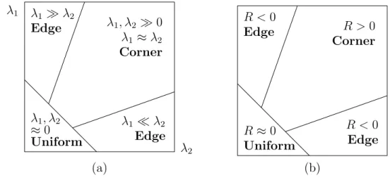
3.2 Analysis of cornerness in the Harris detector. . . 50
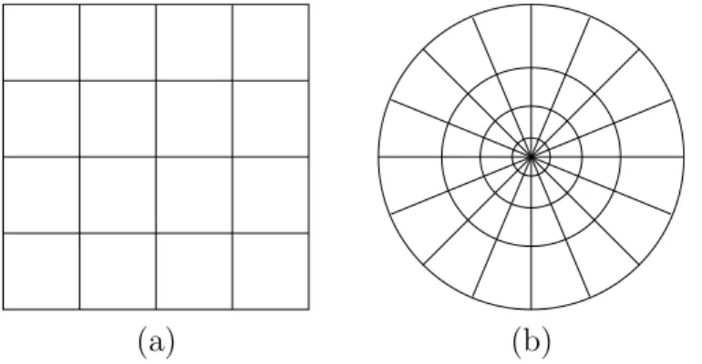
3.3 Commonly used support window spaces. . . 51
3.4 Example of interest point detection. . . 53
3.5 Hierarchical decomposition of an object at several scales. . . 55
3.6 Illustration of the computation of the intrinsic scale for blob features. 55 3.7 Two views of the same object under viewpoint changes. . . 57
3.8 The Gaussian derivatives up to second order. . . 60
3.9 Decompositions of the neighborhood used by SIFT and Shape Context. 61 4.1 Sketch of the learning architecture of RLVC. . . 72
4.2 A percept classifier and its effects on the perceptual space. . . 78
4.3 The different components of the RLVC algorithm. . . 79
4.4 The Binary Gridworld Application. . . 85
4.5 The percept classifier that is obtained at the end of the RLVC process. 86 4.6 Results of RLVC on the Binary Gridworld application. . . 87
4.7 Small visual Gridworld topology. . . 90
4.8 Resolution of the small visual Gridworld by RLVC. . . 90
4.9 Large visual Gridworld topology (with 47 empty cells). . . 91
4.10 A visual, continuous, noisy navigation task. . . 92
4.11 The resulting image-to-action mapping. . . 93
4.12 Representation of the optimal value function. . . 94
4.13 A navigation task with a real-world image. . . 95
5.1 A truth table that defines a mapping f : B4 7→ B. . . . 100
5.2 The Shannon decomposition of a truth table. . . 100
5.3 Normalization of a Shannon decomposition, which produces a BDD. . 101
5.4 The Montefiore campus in Li`ege. . . 106
5.5 An optimal control policy for the Montefiore navigation task. . . 107
5.6 The percepts of the agent. . . 108
5.7 Statistics of RLVC as a function of the step counter k. . . 109
5.8 Statistics of the extended version of RLVC. . . 109 xiii
5.11 The optimal value function that is obtained by RLVC. . . 118
5.12 Two composite components that were generated.. . . 118
5.13 Evolution of the number of times the goal was missed. . . 119
5.14 Evolution of the mean lengths of the successful trials. . . 119
6.1 Assigning a class to an image using a Classification Extra-Tree model. 137 6.2 Computing the state-action utility of a raw percept for a fixed action. 139 6.3 Software architecture for the distributed learning of Extra-Trees. . . . 142
6.4 The sequence of policies πk that are generated by V-API. . . 144
6.5 Error on the generated image-to-action mappings. . . 145
7.1 Illustration of the discretization process of (a) RLVC, and (b) RLJC. 148 7.2 The joint classes that are compatible with a given percept. . . 155
7.3 A path from the root node to an optimal compatible joint class. . . . 157
7.4 A visual, continuous, noisy navigation task with continuous actions. . 162
7.5 The resulting image-to-action mapping. . . 164
4.1 General structure of RLVC . . . 81
4.2 Aliasing Criterion of RLVC . . . 83
4.3 Feature selection process . . . 84
5.1 Refining a BDD-based percept classifier . . . 103
5.2 Compacting a BDD-based percept classifier. . . 104
5.3 Detecting occurrences of visual components . . . 113
5.4 Generation of composite components . . . 114
6.1 Nonparametric Approximate Policy Iteration . . . 131
6.2 Comparison of two state-action value function approximators . . . 132
6.3 Evaluation of a greedy policy in Nonparametric API . . . 133
6.4 General structure for Regression Extra-Tree learning . . . 135
6.5 Recursive induction of a single subtree . . . 135
6.6 Learning oracle for RETQ approximators . . . 140
7.1 General structure of RLJC . . . 154
7.2 Computing the utility of a percept s ∈ S in RLJC . . . 154
7.3 Computing the greedy action π[Q] (s) for some percept s ∈ S . . . 156
7.4 Action seeker for continuous action spaces . . . 158
7.5 Learning a state-action value function that is constrained by Jk . . . 160
7.6 Aliasing Criterion of RLJC . . . 160
7.7 Feature selection process of RLJC . . . 161
Acronyms and abbreviations:
API Approximate Policy Iteration BDD Binary Decision Diagram [Bry92]
DoG Difference of Gaussians (interest point detector) [Low99] LSPI Least-Squares Policy Iteration [LP03]
MDP Markov Decision Process
FMDP Finite Markov Decision Process (state and action spaces are finite) RL Reinforcement Learning [BT96, KLM96, SB98]
RLJC Reinforcement Learning of Joint Classes [JP06] RLVC Reinforcement Learning of Visual Classes [JP05c]
SIFT Scale-Invariant Feature Transform (local descriptor) [Low04] TD Temporal Difference [Sut88]
V-API Visual Approximate Policy Iteration [JBP06]
RETQ Raw Extra-Tree state-action value function approximator General notation:
· 7→ Π(·) probabilistic relation B = {true, false} set of Boolean numbers
G(µ, σ) Gaussian law of mean µ and standard deviation σ
P(·) power set
N set of positive integers
R set of real numbers
R+ set of positive real numbers
R+0 set of positive, non-zero real numbers
x vector
π : S 7→ Π(A) percept-to-action mapping (i.e. probabilistic, Markovian, stationary control policy)
π∗ optimal percept-to-action mapping
A action space (also known as control space)
H Bellman backup operator (cf. Equation 2.26)
Hπ Bellman backup operator for control policy π Qπ(s, a) : S × A 7→ R state-action value function of policy π
Q∗(s, a) : S × A 7→ R optimal state-action value function R(s, a) : S × A 7→ R reinforcement signal
S state space, possibly a set of images
hS, A, T , Ri Markov Decision Process hst, at, rt+1, st+1i interaction
T (s, a, s0) : S × A 7→ Π(S) probabilistic transition relation
T Bellman backup operator (cf. Equation 2.11)
Tπ Bellman backup operator for control policy π Vπ(s) : S 7→ R value function of control policy π
V∗(s) : S 7→ R optimal value function Notation for computer vision:
d(x, y) metric over the visual feature space DL: S 7→ P(R2× W ) interest point detector (cf. Definition 3.3) GL: S × (R2× W ) 7→ V local descriptor generator (cf. Definition 3.5) GV : S 7→ P(V ) visual feature generator (cf. Definition 3.1) Ix (resp. Iy) gradient over the x-axis (resp. y-axis)
of an image I smoothed by a Gaussian
Ixx, Ixy, Iyy second-order derivatives of a smoothed image V visual feature space (usually corresponds to Rn) W support window space (cf. Definition 3.3)
∆t Bellman residual, also known as the
temporal difference at time t (cf. Equation 2.44) A : P(FA) × P(FA) 7→ A action seeker (cf. Definition 7.8)
B b
application of a BDD B to a vector of Booleans b
B(n) family of BDDs with n Boolean inputs
c(k)i perceptual or joint class induced by Ck or by Jk Ck space of joint classes induced by Jk
Ck : S 7→ Sk percept classifier (cf. Definition 4.6) D : (S × A) × F 7→ B joint feature detector
DA: A × FA7→ B action feature detector (cf. Definition 7.1) DV : S × V 7→ B visual feature detector (cf. Definition 4.3) DS : S × FS 7→ B perceptual feature detector (cf. Definition 4.4) F class of state-action value function approximators F = FS∪ FA joint feature space
FA action feature space
FS perceptual feature space
G : P(S × A) 7→ P(F ) joint feature generator
GA: P(A) 7→ P(FA) action feature generator (cf. Definition 7.2) GR: S 7→ P(Rn) raw feature generator (cf. Definition 6.1)
GS : P(S) 7→ P(FS) perceptual feature generator (cf. Definition 4.5) Jk : S × A 7→ Jk joint classifier (cf. Definition 7.6)
L : P(S × A × R) 7→ F learning oracle (cf. Definition 6.3)
ONE
Introduction
Designing robotic controllers rapidly proves to be a challenging problem. Indeed, such controllers (1) face a huge number of possible inputs that can be noisy, (2) must select actions among a continuous set, and (3) should be able to automatically adapt themselves to evolving or stochastic environmental conditions. Although a real-world robotic task can often be solved by directly connecting the perceptual space to the action space through a given computational mechanism, such mappings are usually hard to derive by hand, especially when the perceptual space contains im-ages. Thus, automatic methods for generating image-to-action mappings are highly desirable because many robots are nowadays equipped with CCD sensors.
This class of problems is commonly referred to as vision-for-action. Living beings face vision-for-action problems everyday and learn how to solve them effortlessly and robustly. Despite roughly three decades of research, vision-for-action is still a major challenge in both computer vision and artificial intelligence. A potentially fruitful research path for learning visual control policies1 would therefore be to mimic natural
learning strategies. This dissertation introduces a general framework that is suitable for building image-to-action mappings using fully automatic and flexible learning protocols that resort to reinforcement learning.
1.1
Vision-for-Action
In this dissertation, I am interested in reactive systems that learn to couple visual perceptions and actions inside a dynamic world so as to act reasonably. This coupling is known as a visual (control) policy. This wide category of problems will be called vision-for-action tasks (or simply visual tasks). Despite about fifty years years of active research in artificial intelligence, robotic agents are still largely unable to solve many real-world visuomotor tasks that are easily performed by humans and even by animals. Such vision-for-action tasks notably include grasping, vision-guided navigation and manipulation of objects so as to achieve a goal.
1The terms “visual control policy” and “image-to-action mapping” are used indistinctly.
1.1.1
Reconstructionist Vision
The traditional reconstructionist approach to computer vision is often taken into consideration when solving visual tasks. This paradigm consists in generating a complete, detailed, symbolic 3D model of the surrounding environment [Mar82a]. According to this paradigm, originally proposed by Marr, a computer vision system is a hierarchy of bottom-up processes. Each module in this hierarchy transforms information from an abstraction level into information belonging to a higher ab-straction level. Each abab-straction level comes with its own representation system for encoding the information. The bottom level (the primal sketch) takes raw pixels as input, and generally consists either in the segmentation of the image into regions of interest or in the extraction of visual features (cf. Chapter 3). The top level ulti-mately uses the symbolic representation of the environment so as to choose how to react.
Reconstructionist vision had and still has a great influence on research in com-puter vision. However, it has also been the subject of important criticism:
1. In practice, it is impossible to reconstruct a fully elaborated representation of a visual scene, notably because the projection of a 3D scene into a 2D image causes information loss.
2. Reconstructionist vision systems are rigid, to wit, they are often limited by design to one particular visual task. Moreover, most systems are designed to operate on a fixed set of scenes or objects.
3. The performed task does not weigh in the way the high-level symbolic repre-sentation is built. Thus, even when the model of the environment is computed, a decision making process that may be complex is still needed to choose the optimal reaction.
4. The tasks to be solved are explicitly coded inside the system. Such a task specification is generally difficult to express formally and unambiguously. 5. Many reconstructionist systems are hard-wired and/or do not take lessons
from their prior history, making them unable to improve over time or to adapt to novel situations that were not anticipated by their designers. Many sys-tems also operate under highly controlled conditions and in a fixed context (e.g. exclusively indoor or outdoor, with a known background, and/or without clutter).
These criticisms have motivated the development of alternatives to the reconstruc-tionist paradigm [CRS94]. These alternatives are based on a study of the neuropsy-chological development of the human visual system. The development of sensory-motor coordination of newborns, especially during the first year of life, is indeed a fruitful starting point for biologically-inspired approaches to vision-for-action. Sev-eral facts about this development are outlined in the next section.
1.1.2
Human Visual Learning
An infant is not born perceiving the world as an adult would: The perceptual abilities develop over time. During the first months of life, many cognitive components are either non-functional or not yet fully developed. For example, the control of the ex-tremities is still limited [KBTD95] and the neural growth is not completed [O’L92]. Now, strong neuropsychological evidence suggests that newborns learn to extract useful information from visual data in an interactive fashion, without any external supervisor [GS83]. By evaluating the consequences of their actions on the environ-ment, infants learn to pay attention to visual cues that are behaviorally important for solving their tasks. When they grasp objects, smile or try and reproduce heard sounds, they become aware of the dynamics of the outside world and try to analyze the effects of their reactions in order to improve their behavior.
To this end, the behavior of newborns is optimized for gathering new experi-ences: It favors learning through the collection of data rather than the immediate efficiency of the reactions. Such exploratory behaviors are notably supported by reflexes [PW03]. Even noise can contribute to long-term performance by helping newborns to focus on robust, highly discriminative visual cues. In this manner, as they interact with the outside world, newborns gain more and more expertise on commonplace tasks. Moreover, human visual skills do not remain rigid after child-hood: The visual system continues to evolve throughout life so as to solve unseen visual tasks, and continues to acquire expertise even on well-known tasks [TC03]. Thus, the human visual system is eminently general and adaptive.
Of course, getting representative data for acting efficiently can take a very long time depending on how vast the state space is. This can be particularly problematic in the case of visual tasks. Therefore, infants cannot settle for exploring the environ-ment, but must at some point use the knowledge they have compiled to indeed solve the task. This issue is generally called the exploration-exploitation trade-off [SB98]. Obviously, the process of learning to act in presence of a visual stimulus is task-driven, since different visual tasks do not necessarily need to make the same dis-tinctions [SR97]. As an example, consider the task of grasping objects. It has been shown that, between about five to nine months of age, infants learn to pre-shape their hands using their vision before they reach the object to grasp [MCA+01]. Once
the contact is made, the hand often occludes the observed object so that tactile feed-back is used to locally optimize the grasp. In this context, it is clear that the haptic and the visual sensory modalities ideally complement one another. For this grasp-ing procedure to succeed, infants have to learn to distgrasp-inguish between objects that require different hand shapes. Thus, infants learn to recognize objects according to the needs of the grasping task.
Churchland et al. provide further psychological, anatomical and neuropsycholog-ical evidence for these properties of human visual learning [CRS94]. The lessons above lead to several important conclusions about the criticisms of reconstructionist vision that were drawn at the beginning of this section:
elabo-rated high-level representation of the observed scene. Gathering only a subset of this model might be sufficient for taking optimal decisions in a given visuo-motor task. Human beings build a partial representation of the scene in which only information that is relevant to the performed task is represented.
2. The human visual system is generic and versatile. Its capabilities are not lim-ited by design, but they are generated and augmented as needed: Throughout its entire life, the visual system evolves to acquire additional visual skills. 3. The human visual system is task-dependent , which means that it shortcuts
the visual interpretation process by delivering exactly the information that is needed for solving a given task. In this way, the task directs what information is embedded in the high-level symbolic representations in order to ease the decision making process.
4. The goal of a living being is only implicitly defined (e.g. feeding, fleeing, fight-ing, seeking novelty, experiencing discovery or the survival of the species). This definition partly resorts to pain or pleasure signals that have been hard-wired during the course of evolution.
5. The human visual system is robust and adaptive. These characteristics are closely related to the versatility of human vision. Adaptivity means that ac-quired visual skills are continuously tuned and improved through learning from past experience. This contributes to the improvement of performance, even on well-practiced tasks. This phenomenon is also responsible for the gain in expertise of human vision [TC03]. Expertise rules the recognition of objects at different levels of specificity based on previous experience (e.g. a biologist is able to distinguish between a monkey and a macaque).
Furthermore, it has been argued that the following important properties are inher-ently present in the human visual learning process:
• The learning is interactive, as the consequences of the reactions drive what is learned.
• The learning is exploratory and faces the exploration-exploitation trade-off.
1.1.3
Purposive Vision
Following from the above discussion, a breakthrough in modern artificial intelligence would be to design an artificial system that would acquire object or scene recognition skills based only on its experience with the surrounding environment. To state it in more general terms, an important research direction would be to design a robotic agent that could autonomously acquire visual skills from its interactions with an uncommitted environment in order to achieve some set of goals. Learning new visual skills in a dynamic, task-driven fashion so as to complete an a priori unknown visual task is known as the purposive vision paradigm [Alo90].
Purposive vision is essentially orthogonal to reconstructionist vision. It empha-sizes the fact that vision is task-oriented and that the performing agent should focus its attention only on the parts of the environment that are relevant to its task. For example, if an agent has to move across a maze, it only needs to spot several interesting landmarks; It does not need to be able to recognize all the objects in the environment [Deu04]. Therefore, it is not required to obtain a complete model of the environment. Purposive vision stresses the dependency between action and perception: Selecting actions becomes the inherent goal of the visual sensing pro-cess. This paradigm often leads to the breakdown of the visual task into several sub-problems that are managed by a supervision module that ultimately selects the suitable reactions [Tso94].
The terminology “purposive vision” is somewhat confusing. Purposive vision is indeed very close to active vision [AWB88, BY92, FA95], and these concepts are sometimes used interchangeably. Just like purposive vision, active vision criticizes the passive point of view of reconstructionist vision, and it argues that visual per-ception is an exploratory activity. However, active vision is essentially interested in experimental setups where the position of the visual sensors can be governed by the effectors. This approach is evidently inspired by human vision, for which muscles can orientate the head, the eyes and the pupils. By learning to control such effectors, the agent can acquire better information and resolve ambiguities in the visual data, for example by acquiring images of a scene from different viewpoints. Some ill-posed problems in computer vision become well-posed by employing active vision. An in-stance of an active vision paradigm is Westelius’ robotic arm [Wes95], which uses a focus-of-attention mechanism based on stereo vision. Active vision has also been used in visual navigation for a robot with a stereo active head [Dav98]. However, the paradigm of active vision essentially confines interactivity to the positioning of visual sensors. Thus, purposive vision is more general. Other related paradigms include active perception [Baj88] and animate vision [BB92].
1.2
Objectives
This dissertation attempts to design a general computational framework for purpo-sive vision. More precisely, given the discussion above, my aim is to design machine learning algorithms that can cope with vision-for-action tasks, and that have the following key properties:
• Closed-loop (interactive). The agent should autonomously learn its task by interacting with the environment, without any help from an external teacher or from a supervisory training signal. It should be able to predict the effects of its actions, and to improve them with growing experience.
• Task-driven. The task to be solved should drive which visual skills are learned. • Minimalist. The visual control policies that are learned should not use a complete model of the environment as in reconstructionist vision, but should
rather learn to select discriminative visual cues for the task.
• Integration of time. An action can have a long-term effect on the environment, which must be taken into account when taking a decision. In other words, dynamic environments are considered.
• Versatile. The algorithms should apply to a broad class of vision-for-action problems, should not be tuned for one particular task, and should make few prior assumptions about the tasks and the environment. The same algorithms should be applicable in a variety of environments.
• Implicit formulation of the goal. The objective of the agent should not be hard wired (e.g. in a programming language), but should instead be learned from implicit environmental cues.
This research topic lies at the border between machine learning, computer vision and artificial intelligence. As discussed in the previous section, it can also be mo-tivated from observations of visual neuroscience. The objectives above follow from Piater’s doctoral dissertation [Pia01]. Piater indeed writes:
“Autonomous robots that perform nontrivial sensorimotor tasks in the real world must be able to learn in both sensory and motor do-mains. A well-established research community is addressing issues in motor learning, which has resulted in learning algorithms that allow an artificial agent to improve its actions based on sensory feedback. Little work is being conducted in sensory learning, here understood as the prob-lem of improving an agent’s perceptual skills with growing experience. The sophistication of perceptual capabilities must ultimately be mea-sured in terms of their value to the agent in executing its task.” [Pia01] However, Piater essentially focuses on environments in which an action does not have an impact on the long term. Every time the agent has performed an action, the system is reset, which leads to independent episodes that consists of single decisions. This category of problems is referred to as evaluative feedback by Sutton and Barto [SB98]. Moreover, Piater considers binary tasks, to wit, tasks in which a decision is either correct or wrong. In the framework of this dissertation, there exists a whole continuum in the appropriateness of actions, precisely because the dynamic aspect of the environment is taken into account. Just like in a chess game, a decision with immediate negative consequences (e.g. a sacrifice) may nonetheless later lead to the exploration of highly advantageous parts of the reward space (e.g. winning the game). This general problem that is inherent to dynamic environments is known as the delayed reward problem [SB98].
1.3
Closed-Loop Learning of Visual Policies
One plausible framework to deal with vision-for-action tasks according to purpo-sive vision is Reinforcement Learning (RL) [BT96, KLM96, SB98]. Reinforcement
learning is a biologically-inspired computational framework that can generate nearly optimal control policies in an automatic way, by interacting with the environment2.
RL is founded on the analysis of a so-called reinforcement signal . Whenever the agent takes a decision, it receives as feedback a real number that evaluates the relevance of this decision. From a biological perspective, when this signal becomes positive, the agent experiences pleasure, and we can talk about a reward . Conversely, a negative reinforcement implies a sensation of pain, which corresponds to a punish-ment . Now, RL algorithms are able to map every possible perception to an action that maximizes the reinforcement signal over time. In this framework, the agent is never told what the optimal action is when facing a given percept, nor whether one of its decisions was optimal. Rather, the agent has to discover by itself what the most promising actions are by constituting a representative database of interactions, and by understanding the influence of its decisions on future reinforcements.
1.3.1
Motivation
Reinforcement learning is an especially attractive, well-suited paradigm for closed-loop learning of visual control policies. It is fully automatic, and it fulfills all the six objectives that were stated in Section 1.2 (interactivity, task-driven, minimalism, integration of time, versatility and implicit goal).
Indeed, RL is by definition closed-loop as an optimal visual control policy can be extracted only from a sequence of interactions. It is also task-driven because the learned policy maximizes the reinforcement signal over time, and this signal is of course task-dependent. The generated policies are minimalist as they directly connect a percept to a suitable reaction. The dynamic aspect of the environments is captured since RL does not maximize the immediate rewards, but rather balances immediate rewards with long-term rewards. This is the delayed reward problem that was mentioned at the end of Section 1.2. Reinforcement learning is also a highly versatile paradigm, as it imposes weak constraints on the environment. It can indeed cope with any problem that can be formulated in the framework of Markov Decision Problems. This generic category of problems will be investigated in detail in Chapter2. Intuitively, it corresponds to dynamic environments in which the probability of reaching a state after taking an action is independent of the entire history of the system. Finally, the goal of the agent is only implicitly encoded as a reinforcement signal that the agent struggles to maximize.
Theoretically, it seems natural to directly incorporate image information as the perceptual information of a reinforcement learning algorithm. But this is a diffi-cult task. Directly generating states from image results in huge state spaces, whose size exponentially grows with the size of the perceived images. As a consequence, even standard RL algorithms based on value function approximation (cf. Chapter6) cannot deal with them without making prior assumptions on the structure of the images. Images also often contain noise and irrelevant data, which further
com-2As argued by Sutton [Sut04], the links between RL and Pavlovian conditioning are widely acknowledged [SB90].
plicates state construction. Furthermore, in such huge and noisy state spaces, the reinforcement signal tends to dilute. Because the perceptual space can only be very sparsely sampled, it indeed quickly becomes difficult to guess what is the property of an image that leads to high or low reinforcement. This is the well-known Bellman curse of dimensionality, which makes standard RL algorithms inapplicable to direct closed-loop learning of visual control policies.
The key technical contribution of this dissertation consists in the introduction of reinforcement learning algorithms that can be used when the perceptual space contains images. The algorithms that are developed do not rely on a task-specific pre-treatment. As a consequence, they can be used in any vision-for-action task that can be formalized as a Markov Decision Problem.
It should be noted that in this research, I will take an approach that may seem extremely minimalist. Indeed, no model of the environment will be built at all, and the decisions will only be taken by analyzing the visual stimulus. Thus, the proposed algorithms will learn image-to-action mappings that directly connect an image to the appropriate reaction. This is a direct consequence of the reinforcement learning framework.
1.3.2
Related Work
There exists a variety of work in RL about solving specific robotic problems in-volving a perceptual space that contains images. For instance, Schaal uses visual feedback for solving a pole-balancing task [Sch97]. RL has been used to control a vision-guided underwater robotic vehicle [WGZ99]. More recently, Kwok and Fox have demonstrated the applicability of RL for learning sensing strategies using Aibo robots [KF04]. Paletta et al. learn sequential attention models through reinforcement learning [PFS05]. I also mention the use of reinforcement learning in other vision-guided tasks such as ball shooting [ANTH94], ball acquisition [TTA99], visual ser-voing [GFZ00], robot docking [WWZ04, MMD05] and obstacle avoidance [MSN05]. Interestingly enough, RL is also used as a way to tune the high-level parameters of image-processing applications. For example, Peng and Bhanu introduce RL algo-rithms for image segmentation [PB98], whereas Yin proposes algorithms for multi-level image thresholding, and uses entropy as a reinforcement signal [Yin02].
All of these applications preprocess the images to extract some high-level infor-mation about the observed scene that is directly relevant to the task to be solved and that feeds the RL algorithm. This requires making prior assumptions about the images that will be perceived by the sensors of the agent. The preprocessing step is task-specific and is performed by hand. This contrasts with my objectives, which consist in introducing algorithms able to learn how to directly connect the visual space to the action space, without using manually written code and without relying on a priori knowledge about the task to be solved.
A noticeable exception is the work by Iida et al. who apply RL to seek and reach targets [ISS02], and to push boxes [SI03] with real robots. In this work, raw visual signals directly feed a neural network, and an actor-critic architecture is used to
train the neural network. In these examples, the visual signal is downscaled and averaged into a monochrome (i.e. two-colors) image of 64 × 24 = 1536 pixels. The output of four infrared sensors are also added to this perceptual input. While the approach is effective for the specific tasks, this process can only be used in a highly controlled environment. Real-world images are much richer and could not undergo such a strong reduction in size. Trying to apply this approach to larger images would be fruitless because of the Bellman curse of dimensionality.
In a similar spirit, Ernst et al. have very recently shown the applicability of a novel reinforcement learning algorithm (Fitted Q Iteration [EGW05]) in conjunction with a powerful supervised learning algorithm (Extra-Trees [GEW06]) for closed-loop learning of visual policies when raw image pixels are directly used as the perceptual input [EMW06]. In their experimental setup, an image contains 30 × 30 = 900 grayscale pixels. This method is very close to the algorithm Visual Approximate Policy Iteration (V-API) that will be introduced in Chapter 6, but it has been developed independently and almost simultaneously [JBP06]. Contrarily to V-API, this experimental setup lacks an evaluation on real-world, full-sized images.
Another important, distinct step in the direction of my objectives was achieved by Piater et al., who have considered the aforementioned task of grasping objects by a dexterous manipulator [Pia01, CPG01, PG02]. Starting with the fact that only few pieces of work in robotics combine haptic and visual feedback for grasp-ing [All84,GL86], Piater et al. propose to insert a visual recognition system in front of a grasp controller. This controller, which was initially designed by Coelho and Grupen [CJG97], is purely local and minimizes the wrench residual. The visual recognition system is aimed, given prior haptic experience, at planning an initial grasp that is close enough to the optimal grasp. This initial grasp will be opti-mized through the local controller. In other words, visual feedback ensures the convergence towards an optimum in the space of possible finger configurations. The mappings from images to successful finger configurations are learned through an on-line, incremental protocol [Pia01, Chapter 6]. This process generates discriminative combinations of basic visual features (edgels, texels and salient points), and each of these combinations votes for one configuration of the hand. A Bayesian network is trained to choose the best configuration from these votes. Unfortunately, as men-tioned earlier, this algorithm is only applicable to tasks with two outcomes (the grasp is either successful or not) and in which two successive actions are indepen-dent. This application is therefore inherently closer to supervised learning than to reinforcement learning.
1.3.3
Extraction of Visual Features
The proposed algorithms resort to the extraction of visual features as a way to achieve more compact state spaces that can be used as an input to traditional RL algorithms. Indeed, buried in the noise and in the confusion of visual cues, images contain hints of regularity. Such regularities are captured by the important notion of visual features. Loosely speaking, a visual feature is a representation of some aspect
of local appearance, e.g. a corner formed by two intensity edges, a spatially localized texture signature, or a color. Therefore, to analyze images, it is often sufficient for a computer program to extract only useful information from the visual signal, by focusing its attention on robust and highly informative patterns in the percepts. The program should thereafter seek the characteristic appearance of the observed scenes or objects.
This is actually the basic postulate behind appearance-based vision that has had much success in computer vision applications such as image matching, image re-trieval and object recognition [SM97, Low04]. Appearance-based vision relies on the detection of stable discontinuities in the visual signal thanks to interest point detectors [SMB00,MTS+05]. Similarities in images are thereafter identified using a
local description of the neighborhood around the interest points [MS03, MS05]. If two images share a sufficient number of matching local descriptors, they are con-sidered as belonging to the same visual class. Appearance-based vision is at the same time powerful and flexible as it is robust to partial occlusions and does not require segmentation or 3D models of the scenes. Mikolajczyk et al. provide a list of successful applications of appearance-based vision [MS05].
Intuitively, appearance-based vision allows the extraction of a maximum amount of relevant information from the images, while keeping the amount of data man-ageable. Interestingly enough, Paletta et al. have also exploited visual features in the context of reinforcement learning for optimizing sensorimotor behavior in the context of active vision [PRB05, PFS05].
1.3.4
Task-Driven Exploitation of Visual Features
It seems therefore promising to use the visual feature space instead of the raw images as the input to the reinforcement learning algorithms. Indeed, visual features are vectors that are composed of about a hundred components, which contrasts with the typical images that contain hundreds of thousands of pixels. Thus, reinforcement learning seems easier to carry out in this visual feature space. Nevertheless, many features can be extracted from a single image. In other words, the extraction of visual features from an image is a one-to-many mapping. Thus, the main challenge of the algorithms that will be developed is to determine which, among the many visual features it perceives, are the ones relevant to the reward or punishment.
In this dissertation, two ways to deal with this abundance of visual features are investigated. The first possibility is to select the visual features that are the most discriminative for the performed task . This basic idea has already been investigated by McCallum’s U Tree algorithm [McC96]. This algorithm will be adapted to visual tasks in the Reinforcement Learning of Visual Classes algorithm. The name of the algorithm comes from the fact that the visual space is discretized into a small set of visual classes by testing the presence of those highly discriminative visual features. The second possibility is to use the whole set of raw visual features, without selecting the most discriminative ones. This is motivated by the fact that even less discriminative features can have an impact on the optimal decisions. Instead
of creating a set of visual classes, low-level vectors of real numbers that encode the visual features are directly used. As visual data can be sampled only sparsely, function approximators will be embedded inside the RL process. These ideas will lead to the development of the Visual Approximate Policy Iteration algorithm.
It is important to realize that the visual feature space can be composed of raw pixels. Indeed, the extraction of visual features can consist in the selection of infor-mative patches in the image and in the description of each of those patches as the set of raw pixels they contain. Furthermore, the extraction of visual features can gener-ate a single visual feature for each image. Therefore, the introduced framework can deal with the same perceptual spaces as those considered by Iida et al. [ISS02,SI03] and Ernst et al. [EGW05] (cf. Section 1.3.2).
1.4
Outline of the Dissertation
This dissertation targets the development of algorithms that make reinforcement learning computationally tractable on complex, high-dimensional visual tasks. In a nutshell, the basic idea is to take advantage, in an automatic way, of visual features that are borrowed from appearance-based vision. The results of this dissertation unify those appearing in previous publications [JP04,JP05a,JP05b,JP05c,JP05d,
JP05e, JSP05, JBP06,JP07, JP06].
Each algorithm that will be introduced in the sequel comes from a practical consideration that was guided by the experiments. Ideas from experiments and programming influenced the theoretical development, and vice versa. This goal-driven approach turned out to be very fruitful. The development of software in the C and in the C++ programming languages forms a major part of my work. The main developments were: (a) a core object-oriented library for reinforcement learning that supports vision-for-action tasks and that is used throughout the experiments; (b) a library for the learning of classification and regression trees, and notably Extra-Trees [GEW06]; (c) a library for distributed computing of bag-of-tasks on a cluster of computers; and (d) the data distribution of a database through the BitTorrent protocol [Coh03].
This dissertation is organized as depicted in Figure 1.1. Because the topic of this research work is at the crossroads of computer vision and machine learning, this dissertation begins with two background chapters that present the state of the art of the two main theoretical tools that will be used:
• In Chapter 2, the basic results from the theory of reinforcement learning are presented. The formalism that is used throughout this dissertation is in-troduced. Theoretical foundations of RL are discussed, as well as standard algorithms. This chapter makes no assumptions abouth the state and ac-tion spaces, except that they must both be finite. Visual state spaces are not considered in this part of the dissertation. People from the computer vi-sion community might find this an useful introduction to the vivi-sion-for-action paradigm.
Purposive vision Vision-for-action
(Chapter 1)
Reinforcement learning
(Chapter 2) Appearance-based vision(Chapter 3)
Nonparametric Approximate Policy Iteration (Chapter 6.3) Reinforcement Learning of Visual Classes (Chapter 4) Visual Approximate Policy Iteration (Chapter 6.5) Reinforcement Learning of Joint Classes (Chapter 7) Function approximators (Chapter 6.2) Distributed implementation of Extra-Trees (Chapters 6.4 and 6.6) continuous actions Closed-loop learning of
hierarchies of visual features (Chapter 5.2) Fighting overfitting
in RLVC (Chapter 5.1)
Figure 1.1: Synoptic view of this dissertation. Arrows represent the dependencies between the various concepts that are introduced in the chapters. My personal contributions are highlighted in green. The Extra-Trees learning algorithms result from research work by Geurts et al. [GEW06], but the distributed implementation of Extra-Trees is a personal contribution.
• Chapter3introduces appearance-based vision along with visual features. The central notion of a visual feature generator is introduced. Then, global-ap-pearance methods and local-apglobal-ap-pearance methods are both discussed, the latter being defined as the conjunction of an interest point detector with a local description generator . This introductory chapter concludes by showing how visual features are used in typical computer vision applications. Some precise insight on how visual features could be used when solving vision-for-action tasks are also given. This discussion should be mostly helpful to people from the machine learning community.
After these two background chapters, the remaining chapters constitute the heart of this dissertation. These technical chapters share the same general structure: The precise problem and the proposed solution are stated, the related work is discussed, novel algorithms are formally derived, experimental results are presented, and a discussion concludes. The validity of the proposed methods are demonstrated on vision-guided navigation tasks. Here are the contributions that will be described:
• The Reinforcement Learning of Visual Classes (RLVC) algorithm is derived in Chapter 4 by building on the visual feature space defined in the preceding chapter. As mentioned earlier, this algorithm selects highly informative visual features in an incremental process.
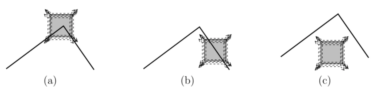
• Chapter 5 presents two extensions to RLVC. The first extension consists in reducing the overfitting that is inherent to RLVC by resorting to techniques borrowed from computer-aided verification. Although this process is more resource consuming, it is useful to ensure better convergence properties. The second extension is closely related to Scalzo’s research work [SP05,SP06], and proposes algorithms to generate a hierarchy of spatial combinations of visual features that are more and more discriminative. This process proves to be useful when individual features are not informative enough to solve a vision-for-action task. This is illustrated on a visual version of a classical control problem (the car-on-the-hill task).
• The Visual Approximate Policy Iteration (V-API) algorithm is introduced in Chapter 6. As mentioned earlier, this algorithm uses the raw visual features through a function approximation scheme. This chapter notably introduces the Nonparametric Approximate Policy Iteration algorithm, that is a generic version of the Least-Squares Policy Iteration algorithm [LP03]. The supervised learning of Extra-Trees [GEW06] is also described, as it is a main component of V-API. This chapter also shows how to distribute the generation of Extra-trees among a cluster of computers so as to dramatically reduce the computational requirements.
• All the algorithms from the previous chapters are defined on finite action spaces. Chapter 7 generalizes RLVC to continuous action spaces, leading to the more general Reinforcement Learning of Joint Classes (RLJC) algorithm.
This is useful, as robotic controllers often interact with their environment through a set of continuously-valued actions (position, velocity, torque. . . ). RLJC adaptively discretizes the joint space of visual percepts and continuous actions, which is in essence a novel approach.
Finally, Chapter8 concludes this dissertation with a summary of the main con-tributions and with a discussion of possible future directions.
TWO
Reinforcement Learning
Reinforcement Learning (RL) is concerned with the closed-loop learning of a task within an a priori unknown environment. The learning agent takes lessons from a sequence of trial-and-error interactions with the surrounding environment. In RL, the task to be solved is not directly specified. Instead, whenever the agent takes a decision, it feels either pain or pleasure. This so-called reinforcement signal implicitly defines the task. The goal of the agent is to learn to act rationally, that is, to learn how to maximize its expected rewards over time. RL algorithms achieve this objective by constructing control policies that directly connect the percepts of the agent to the suitable reaction when facing these percepts.
The agent is never told the best reaction when facing a given situation, neither whether it could reach better performance than the one it currently achieves. As a consequence, RL schematically lies between supervised learning and unsupervised learning. Indeed, in supervised learning, an external teacher always gives the correct reaction to the agent and the agent has to learn to reproduce the given input-output relation. On the other hand, the unsupervised learning protocol gives strictly no clue about the goodness of the decisions: The agent has to structure its percepts without getting feedback. The major advantages of the RL protocol are that it is fully automatic, and that it imposes only weak constraints on the environment.
As a consequence, RL can be distinguished from other learning paradigms by three main characteristics:
1. the implicit definition of a goal through reinforcements,
2. the temporal aspect of the task (a decision can have a long-term impact, both on the system dynamics and on the earned rewards), and
3. the trial-and-error learning protocol (which contrasts with supervised and un-supervised learning).
In this chapter, RL is introduced. Note that many textbooks present a more thorough coverage of the fields of reinforcement learning and its relation to the theory of dynamic programming [KLM96, BT96, SB98].
2.1
Markov Decision Processes
Reinforcement learning is traditionally defined in the framework of Markov Deci-sion Processes (MDP). Bellman founded the theory of MDPs [Bel57a, Bel57b] by unifying previous work about sequential analysis [Wal47], statistical decision func-tions [Wal50], and two-person dynamic game models [Sha53].
The current section presents a self-contained introduction to finite Markov de-cision processes. The theorems that are useful in reinforcement learning for finite state-action spaces will be formally derived. The only statement that will not be proved is the Bellman optimality theorem (Theorem2.15). Our aim is to emphasize how the main results about MDPs can be derived starting from the latter theorem. The components that make up an MDP are rigorously defined in the subse-quent sections. Notation that is similar, but not identical to that of Sutton and Barto [SB98], will be used.
2.1.1
Dynamics of the Environment
A Markov decision process is a stochastic control system whose state changes over time according to discrete-time dynamics, and whose evolution can be controlled by taking a sequence of decisions. Therefore, the trajectory that is followed by the system depends on the interactions between the “laws of motion” of the system and the decisions that are chosen over time.
At any time t = 0, 1, . . ., the system can be observed and classified into one state st of a set of states S. At any time t, the learning agent influences its environment by taking one action at of a set of actions A, hereby controlling the system. The laws of motion of the MDPs are assumed to be governed by a time-invariant set of transition probabilities. The probability of reaching a state st+1 after applying the action at in the state st does not depend on the entire history of the system, but only on the current st and at:
P st+1 = s | s0, a0, s1, a1, . . . , st, at | {z }
history of the system
= P{st+1= s | st, at}. (2.1)
This strong assumption on the system dynamics is generally known as the Markov hypothesis. Thus, the dynamics of MDPs can be entirely specified by defining a probabilistic relation T that links st, at and st+1:
T (s, a, s0) = P{st+1= s0 | st= s, at= a}. (2.2) Of course, the Markov hypothesis has many interesting implications that will be investigated in the next sections. Note however that despite the Markov hypothesis, an action can have a long-term impact on the trajectory of the system, and that the outcome of a decision is generally not perfectly predictable, because of the stochastic aspect of T .
2.1.2
Reinforcement Signal
In MDPs, the control law that has to be learned is not directly specified. Rather, it is defined implicitly through a reinforcement signal that provides a quantitative evaluation of the reactions of the learning agent. Every time it takes a decision, the agent receives either a reward or a punishment, depending on its performance. So, the reinforcement signal tells which task is to be solved, but not how to solve the task. From a biological perspective, the reinforcement signal corresponds to pleasure or pain feelings that living beings may perceive while learning to achieve a task.
Concretely, at each time stamp t, the agent receives a real number rt+1 = R(st, at), that is called the reinforcement at time t + 1 and that depends on the state st and on the action at that was performed in this state. In this framework, costs can be encoded as negative rewards.
Markov Decision Processes can now be formally defined as the assembly of a Markovian dynamics with a reinforcement signal:
Definition 2.1. A Markov Decision Process (MDP) is a quadruple hS, A, T , Ri, where:
• S is a set of states, • A is a set of actions,
• T : S × A 7→ Π(S) is a probabilistic transition relation from the state-action pairs to the states, and
• R : S × A 7→ R is the reinforcement signal that maps a state-action pair to a real number.
Remark 2.2. In this definition, the notation R : E 7→ Π(F ) is employed to desig-nate a probabilistic relation R that maps a set E to a set F . Thus, R is a probability density function over the Cartesian product E × F . 2
A very important subclass of Markov decision processes is constituted by those MDPs whose set S of states and set A of actions are both finite:
Definition 2.3. A Finite Markov Decision Process (FMDP) is a Markov decision process hS, A, T , Ri such that S and A are finite sets.
2.1.3
Histories and Returns
As the agent interacts with its environment, the MDP describes a trajectory in the set of states. This trajectory depends on the actions that are chosen by the agent. So, the whole history of an MDP is a sequence of state-action pairs that is composed of the states that have been visited so far and of the previous actions that have been chosen when facing these states:
Definition 2.4. The history of an MDP up to time stamp t ≥ 0 is a sequence ht= (s0, a0, s1, a1, . . . , st−1, at−1, st). The set Ht of possible histories up to t is:
Ht = (S × A)t× S, (2.3)
and the set H of all possible histories is: H = [ t∈N Ht = [ t∈N (S × A)t× S. (2.4)
To each history ht ∈ Ht corresponds a sequence r0, r1, . . . , rt−1 of earned rein-forcements, where rk = R(sk, ak) for all k < t. Importantly, the immediate reward or punishment can be the consequence of decisions that were made long before. In other words, the reinforcements can be delayed . Therefore, the actions cannot be viewed independently of each other, and the agent may face a dilemma: Taking a less immediately attractive action can enable the agent to reach parts of the state space of the MDP where it can get higher future reinforcements. This makes for example particular sense when modeling two-person games such as chess, in which sacrificing a piece might lead to an advantage later in the game, or when modeling robotic tasks, in which each elapsed period of time induces a cost. Thus, the agent must balance its propensity for acquiring high immediate reinforcements with the possibility of earning higher rewards afterward.
Consequently, the concept of returns is introduced, that embodies this trade-off the learning agent has to make between present and future reinforcements. Given an infinite history h ∈ H∞ of the interactions of the agent with the MDP, the corresponding return is the cumulative sum of reinforcements over time:
Definition 2.5. The (discounted) return R(h) that is collected during an infinite history h ∈ H∞ is: R(h) = ∞ X t=0 γtR(st, at), (2.5)
where γ ∈ [0, 1[ is the discount factor . Such a series always converges.
The temporal discount factor γ gives the current value of the future reinforcements. From a financial point of view, γ corresponds to the time value money, that is one of the basic concepts of finance: Money received today is more valuable than money received in the future by the amount of revenues it could yield. As it is assumed that γ < 1, the effect of distant future reinforcements becomes negligible. To intuitively paraphrase this definition, as future decisions influence the benefits of the current decision, the definition of discounted return stresses the short-term rewards, without totally neglecting the long-term consequences.
Note that as γ tends to 1, the agent takes long-term consequences more strongly into account. Conversely, if γ = 0, the agent is myopic and only tries to maximize its immediate reinforcements1
2.1.4
Control Policies
The agent interacts with the MDP through its effectors by taking actions. Whenever the agent faces some state, it must choose a suitable action according to the history of the system. The internal process of choosing actions is captured by the notion of decision rule:
Definition 2.6. A decision rule δ : H 7→ Π(A) is a probabilistic mapping from the set of possible histories to the set of actions.
A decision rule δ(ht, at) tells the agent the probability with which it should choose an action at ∈ A if the history of the system is ht∈ Ht at a given time stamp t. To control the system over time, a sequence of such decision rules must be used, one for each time stamp:
Definition 2.7. A general control policy π is an infinite sequence of decision rules: π = (δ0, δ1, . . . , δt, . . .).
The primary objective of the theory of MDPs is to find general control policies that are optimal for a given MDP, in a sense that remains to be defined.
Three very important subclasses of general control policies are now discussed. Firstly, a general control policy is Markovian if the decision rules do not depend on the whole history of the system, but only on the current state st:
Definition 2.8. A general control policy π = (δ0, δ1, . . . , δt. . .) is Markovian (or memoryless) if, for each time stamp t, there exists a probabilistic mapping δt0 : S 7→ Π(A) such that δt(h) = δt0(st) for all h = (s0, a0, . . . , st) ∈ Ht.
Markovian control policies are particularly attractive, as the agent is not required to memorize the entire history of its interactions with the environment to choose the dictated action. Intuitively, it seems natural to only consider Markovian control policies when solving MDPs because the dynamics of MDPs is itself Markovian. This insight will be confirmed later.
Secondly, if the same decision rule is used at each time stamp, the general control policy is called stationary:
Definition 2.9. A general control policy π = (δ0, δ1, . . . , δt, . . .) is stationary (or time invariant ) if δi = δj for all i, j ∈ N.
Evidently, any decision rule δ can be extended to a control policy π = (δ, δ, . . . , δ, . . .). Finally, if each decision rule defines a single-valued transform from the states to the actions, the general control policy is called deterministic:
Definition 2.10. A general control policy π = (δ0, δ1, . . . , δt. . .) is deterministic if, for each time stamp t and each possible history ht ∈ Ht, there exists one action at such that δt(ht, at) = 1.
As a shorthand, if π is deterministic, the notation δt(ht) will refer to the action that is selected with probability 1 by the decision rule δtif faced with the history ht∈ Ht.
Remark 2.11. If a policy π is at the same time Markovian and stationary, the policy collapses to a probabilistic mapping S 7→ Π(A) from the states to the actions. In such case, π(s, a) will designate the probability of choosing action a ∈ A when facing some state s ∈ S. If π is moreover deterministic, π(s) will refer to the action that is selected with probability 1. 2
2.1.5
Value Functions
Suppose that, starting in a particular state, actions are taken following a fixed control policy. Then the expected sum of rewards over time is called the value function of the policy that is followed. More precisely, each general control policy π is associated with a value function Vπ(s), that gives for each state s ∈ S the expected discounted return obtained when starting from state s and thereafter following the policy π: Definition 2.12. The value function Vπ : S 7→ R of a general control policy π for any state s ∈ S is:
Vπ(s) = Eπ{R(h) | s0 = s} = Eπ ( ∞ X t=0 γtR(st, at) | s0 = s ) , (2.6)
where Eπ denotes the expected value if the agent follows π, starting with an history h0 that only contains s. Vπ(s) is called the utility or the value of the state s under the policy π.
Evidently, the value function for a given general control policy is by definition unique. It is now proved that value functions of Markovian, stationary control policies satisfy a very specific recursive relation in finite MDPs. This property expresses a relationship between the value of a state and the values of its successor states:
Theorem 2.13 (Bellman equation). Let π be a Markovian, stationary control policy for a finite MDP hS, A, T , Ri. Using the notation from Remark2.11, we get:
Vπ(s) =X a∈A π(s, a) R(s, a) + γX s0∈S T (s, a, s0)Vπ(s0) ! , for each s ∈ S. (2.7)
Proof. The proof is given in AppendixA. 2
If the considered policy is also deterministic, this theorem can be readily special-ized as:
Corollary 2.14. If π is a Markovian, stationary, deterministic control policy in a finite MDP, then:
Vπ(s) = R(s, π(s)) + γX s0∈S
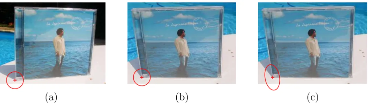
![Figure 3.4: Example of interest point detection. (a) An illustrative image that is taken from the database that has been collected for this research work [Jod05].](https://thumb-eu.123doks.com/thumbv2/123doknet/6205744.160276/73.893.225.681.167.945/figure-example-point-detection-illustrative-database-collected-research.webp)
![Figure 4.2: A percept classifier and its effects on the perceptual space. (This illus- illus-tration is strongly inspired by Pyeatt and Howe [PH01].)](https://thumb-eu.123doks.com/thumbv2/123doknet/6205744.160276/98.893.232.649.144.459/figure-percept-classifier-effects-perceptual-tration-strongly-inspired.webp)
![Figure 4.4: On the left, Sutton’s Gridworld [Sut90]. Filled squares are walls, and the exit is indicated by an asterisk](https://thumb-eu.123doks.com/thumbv2/123doknet/6205744.160276/105.893.130.761.157.305/figure-sutton-gridworld-filled-squares-walls-indicated-asterisk.webp)

