HAL Id: pastel-00785349
https://pastel.archives-ouvertes.fr/pastel-00785349
Submitted on 6 Feb 2013
HAL is a multi-disciplinary open access archive for the deposit and dissemination of sci-entific research documents, whether they are pub-lished or not. The documents may come from teaching and research institutions in France or abroad, or from public or private research centers.
L’archive ouverte pluridisciplinaire HAL, est destinée au dépôt et à la diffusion de documents scientifiques de niveau recherche, publiés ou non, émanant des établissements d’enseignement et de recherche français ou étrangers, des laboratoires publics ou privés.
Study of the diffusion, rheology and microrheology of
complex mixtures of bacteria and particles under flow
confined in thin channels.
Gaston Miño
To cite this version:
Gaston Miño. Study of the diffusion, rheology and microrheology of complex mixtures of bacteria and particles under flow confined in thin channels.. Soft Condensed Matter [cond-mat.soft]. Université Pierre et Marie Curie - Paris VI, 2012. English. �pastel-00785349�
DOCTORAL THESIS
UNIVERSITE PIERRE ET MARIE CURIE
Speciality: Physique
Doctoral School: "ED P2MC 389"
made in
École supérieure de physique et de chimie industrielles
Physique et Mécanique des Milieux Hétérogènes
presented by
Gastón Leonardo MIÑO
to obtain the degree of
DOCTOR FROM PIERRE AND MARIE CURIE UNIVERSITY
title of the thesis
Study of the diffusion, rheology and microrheology of
complex mixtures of bacteria and particles under flow
confined in thin channels.
Presented 10 February 2012, Paris.jury composed by:
Pr. Wilson Poon Referee
Pr. Hartmut Löwen Referee
Pr. Jean-Francois Joanny Examiner
Pr. Philippe Peyla Examiner
Résumé
Pour ma thèse, j’ai étudié trois problèmes autour des propriétés de transport des sus-pensions actives. J’ai utilisé principalement des sussus-pensions de bactéries Escherichia Coli mais aussi des systèmes de nageurs artificiels auto-propulsés.
En premier lieu, j’ai étudié l’activation du mouvement Brownien de particules passives dans une suspension de bactéries, près d’une surface. En utilisant diverses solutions et diverses conditions expérimentales permettant de changer les conditions de nage des bactéries et le confinement, j’ai montré que la diffusivité des traceurs pas-sifs augmente linéairement avec ce que j’ai défini comme le flux actif de la suspension; c’est à dire la concentration de nageurs actifs multipliée par leur vitesse moyenne de nage. De manière générale, le confinement entre deux parois ou par rapprochement d’une paroi, montre un meilleur transfert de la quantité de mouvement qui a pour conséquence une augmentation du facteur de couplage entre diffusivité et fluide ac-tif. Le remplacement des bactéries par des nageurs artificiels comme des bâtonnets bi-métalliques en condition réductrice produit des résultats identiques.
Deuxièmement, j’ai étudie la modification de la viscosité d’un fluide produite par la présence d’entités autopropulsées. Il a été montré théoriquement que la présence de nageurs du type "pousseurs" comme les bactéries, réduit la viscosité de la suspension à une valeur inférieure de celle du fluide porteur. Le manque de résultats expérimen-taux qui mettent en évidence cet effet au sein d’une suspension (cela été montré pour des films liquides minces), nous a poussé à fabriquer un rhéomètre microfluidique en forme d’Y permettant d’étudier la réponse rhéologique d’une suspension d’E. Coli. Des résultats préliminaires révèlent un comportement non Newtonien de la suspen-sion active avec une baisse de viscosité du liquide aux faibles taux de cisaillement et aux faibles fractions volumiques.
Troisièmement, j’ai propose d’étudier les effets de dispersion et de transport de solutions E. Coli dans un micro canal rectangulaire possédant une constriction en
son centre. Dans un tel milieu confiné, les interactions avec les parois ainsi que la géométrie du canal jouent un rôle essentiel sur les propriétés de transport. Mes ré-sultats, de façon inattendue, montrent que l’écoulement dans un canal produit une re-concentration en bactéries après la constriction et que cet effet est contrôlé par l’écoulement même.
Abstract
In my thesis, I studied three problems involving E. Coli bacterial suspensions.
Firstly, I focused on the Brownian motion of passive tracers in this particular ac-tive suspension close to a surface. Buoyancy and non-buoyancy swimming solutions were tested, revealing a linear increase of the passive tracer diffusion with the "active flux", obtained by the active concentration of bacteria multiplied by the mean veloc-ity. Boundary confinements were also explored in buoyancy conditions, showing a better momentum transfer of the active bacteria as the height of the confinement gets smaller. The use of artificial swimmers instead of bacteria also leads to similar results in the enhancement of the diffusion.
Secondly, I considered the modification of the fluid viscosity caused by the pres-ence of these self-propelling entities. It is known that for pusher swimmers as bacteria the viscosity can even be smaller than that of the suspending fluid viscosity. The lack of experimental result showing this effect in the bulk inspired us to build a Y shape micro-fluidic channel in order to study the rheology of wild type E. Coli suspension. Preliminary results show a non-Newtonian behavior of active solution with a decrease of the liquid viscosity at low volume fractions and low shear rates.
Thirdly, I proposed to address the question of dispersion and transport of E. Coli suspensions flowing in a micro-channel with a constriction. Here, in a confined en-vironment , the interactions with the boundaries and the geometry of the channels play an essential role. Surprisingly, my results show that the flow in a channel can produce a re-concentration of bacteria after passing through the constriction and this can be controlled by the flow.
Acknowledgement
It took me three years to reach this point in my life and to achieve this goal. Several persons have been involved in this process.
First and foremost, I owe a lot to my supervisor Eric Clément who has given me the opportunity to work with him. I thank him for his stimulating suggestions and encouragement. He has helped me immensely during the research for and the writing of this thesis. I also would like to express my gratitude to Dr Annie Rousselet and thank her for sharing her knowledge and for supervising my work. Without her guidance and help this work would not have been possible. I would like to thank Dr José Eduardo Wesfreid for being the "bridge" that brought me to PMMH.
I also want to thank Mr. Jérémie Gachelin, Ing. Thierry Darnige, Dr. Mauricio Hoyos , Hélène Berthet, and Dr. Anke Lindner. These PMMH co-workers have had an active participation during these three years, have helped me and I have had enriching discussions with them. I would like to thank the staff of PMMH and all my colleagues for making my stay comfortable and for making me feel welcome.
Gracias Ms Jocelyn Dunstan and Pr Rodrigo Soto from the Chile University for all the scientific discussions, support and also for the warm welcome received every time that I visited their lab in Chile. Gracias to Pr. Ernesto Altshuler from the Uni-versity of Havana for working with me and for sharing many hours of discussion and laboratory work. I would like to thank Pr Thomas Mallouk from Penn State who helped me during his sabbatical at the École Normale Supérieure in 2009-2010 with the realization of part of my work presented in this thesis.
This thesis would not have been possible without the financial support of Founda-tion Pierre-Gilles de Gennes.
I want to express my profound gratitude to a college and very good friend, Dr Veronica Raspa. I thank her for being at my side, for encouraging and supporting me, especially at the last stages of this thesis.
Because they are with me for each step that I take, they support me and are by my side no matter the distance, I want to express my gratitude and love to my Family and Friends in Paraná, Argentina.
Finally, I want to thank someone very important to me and on whom I can count whenever I need to: Thank you Jochen.
Contents
1 Introduction 5
I
Active Brownian motion
15
I.1 Methodology and Protocol 16
I.1.1 Experimental Setup . . . 17
I.1.1.1 Hydrodynamic trapping at the walls . . . 21
I.1.2 Experimental characterization of bacteria trajectories at the walls . . . . 25
I.1.2.1 Bacteria Detection . . . 25
I.1.2.2 Bacteria Tracking and Trajectory Analysis . . . 27
I.1.2.3 Population Motility Characterization . . . 32
I.1.3 Motion of Passive Tracers . . . 37
I.2 Diffusion enhancement 44 I.2.1 Diffusion enhancement in non-buoyant condition . . . 45
I.2.2 Diffusion enhancement in buoyant condition . . . 47
I.2.2.1 Varying the swimmer velocity . . . 48
I.2.2.2 Varying the wall confinement . . . 49
I.2.3 Artificial Swimmers . . . 52
II
Swimmers in a flux
59
II.1Active viscosity of E. Coli suspensions 60 II.1.1 Operation principles . . . 61II.1.2 Methodology and Protocol . . . 63
CONTENTS 2
II.1.2.1 Experimental Setup . . . 63
II.1.2.2 Image Analysis . . . 65
II.1.3 Quality test of the channel . . . 66
II.1.4 Experimental results . . . 68
II.1.4.1 Passive Particles . . . 68
II.1.4.2 Bacterial Suspension: Dead Bacteria . . . 70
II.1.4.3 Bacterial Suspension: Living Bacteria . . . 71
II.2Anomalous dispersion of a confined bacterial flow 76 II.2.1 Methodology and Protocols . . . 77
II.2.1.1 The micro-fluidic funnel . . . 77
II.2.1.2 Experimental setup and procedure . . . 78
II.2.2 Experimental results . . . 80
II.2.2.1 Flow induced symmetry breaking . . . 80
II.2.2.2 Effect of flow reversal on symmetry breaking . . . 83
II.2.2.3 Evidence of long range anomalous dispersion . . . 84
II.2.2.4 Qualitative scenario for symmetry breaking . . . 87
II.2.2.5 Trapping/untrapping at the lateral walls . . . 88
General Conclusion 92
Appendix 99
List of Figures
1.1 Eschericha Coli scheme. . . 6
1.2 Puller and Pusher effect in the surrounding fluid. . . 7
1.3 Puller and Pusher effect in the surrounding fluid. . . 8
1.4 Mean Square Displacement (MSD) of passive tracer in a bacterial sus-pension film. . . 9
1.5 Active contribution in the fluid viscosity presented by Saintillan (2010). 10 1.6 Active contribution in the fluid viscosity presented by Ryan et al. (2011). 10 1.7 Effect on the viscosity for pusher-like swimmers. . . 11
1.8 Effect on the viscosity for puller-like swimmers. . . 11
1.9 Active density control presented by Galadja et al. (2007). . . 12
1.10 Sorting device presented by Hulme et al. (2008). . . 13
I.1.1 Experimental Setup for Passive Particles Activation . . . 18
I.1.2 Bacterial profile in a buoyancy and "non-buoyancy" conditions. . . 19
LIST OF FIGURES 1
I.1.4 Two-sphere model for bacteria. . . 22
I.1.5 Behaviors in a Two-sphere model. . . 23
I.1.6 Bacteria visualization at different height . . . 25
I.1.7 Image processing to recognize bacterial positions . . . 26
I.1.8 Bacterial Trajectories . . . 27
I.1.9 Definition of θ that will give the mean persistence angle | <θ >| for the trajectory. . . 28
I.1.10 Definition of L for both type of motion. . . 28
I.1.11 Density probability of the observed bacterial tracks . . . 30
I.1.12 Identification of the bacterial population . . . 31
I.1.13 MSD calculated for bacteria . . . 32
I.1.14 Diffusion Distribution for random bacteria . . . 33
I.1.15 Velocity and Diffusion Distribution for Bacteria . . . 34
I.1.16 Relation between the active swimmer’s mean velocity VA and φA . . . 35
I.1.17 Circular Trajectory Fitting . . . 36
I.1.18 Radius distribution . . . 36
I.1.19 Radius as function of the velocity . . . 37
I.1.20 Image analysis for passive tracers . . . 38
I.1.21 Passive Tracer Trajectories. . . 38
I.1.22 Means Square Displacement (MSD) of a passive particle . . . 39
LIST OF FIGURES 2
I.1.24 Passive Tracer trajectories under a drift. . . 41
I.1.25 Passive Tracer Diffusivity computed using the six different methods. 42 I.2.1 Enhanced diffusivity DP of passive tracers as a function of JAin non-buoyancy conditions. . . 46
I.2.2 Effect of the pH in mean velocity VA of the active population using MMA solution. . . 48
I.2.3 Enhanced diffusivity DPof passive tracers as a function of JAin buoy-ancy conditions . . . 49
I.2.4 Schematic of the chamber used to vary the distance between bottom and top walls. . . 50
I.2.5 Effect of confinement on the Brownian diffusion of passive tracers. . . 50
I.2.6 Effect of the confinement in the β1/4 value. . . 51
I.2.7 Scheme of Au/Pt rod and its field emission scanning electron mi-croscopy image. . . 53
I.2.8 Scheme of the setup used in the Au/Pt rod experiments. . . 54
I.2.9 Two experiment using a mixture of Au rods and Au/Pt rods. . . 55
I.2.10 Velocity and diffusion distribution for active and random rods . . . . 56
I.2.11 Relation between mean velocity of active swimmer VAand active frac-tion φA for Au-Pt rods. . . 57
I.2.12 Enhance diffusion in suspensions of Au-Pt rods. . . 58
II.1.1 Experimental setup in the Y-Shape experiment. . . 62
LIST OF FIGURES 3
II.1.3 Image analysis for the interface determination in a Y-shaped channel. 65
II.1.4 Quality test of the Y-shape Viscosimeter at a flow equal to 1 nl/s. . . 66
II.1.5 Quality test of the Y-shape Viscosimeter at a flow equal to 10 nl/s. . . 67
II.1.6 Quadratic width σ2 of the fitting er f function for different volume fractions. . . 69
II.1.7 Viscosity results in a suspension of passive particles using Y-shape microchannel. . . 70
II.1.8 Relative shear stress (Σr) as a function of the mean shear rate ( ˙γ). . . 71
II.1.9 Relative viscosity as a function of volume fractions using dead bacteria. 72 II.1.10 Channel images at the different shear rates for alive bacteria . . . 73
II.1.11 Rheology measurement for living bacteria suspensions. . . 74
II.2.1 Scheme of the experimental setup using a funnel. . . 77
II.2.2 Photography of the microchannel developed by soft Lithography. . . 78
II.2.3 Definition of the areas at both sides of the constriction. . . 80
II.2.4 Flow-controlled symmetry breaking in the concentration of E. Coli. . 81
II.2.5 Trajectory tracks of 1 second duration at different mean fluid velocities. 82 II.2.6 Time evolution of n(t). . . 84
II.2.7 Different moments in the flow reversibility . . . 85
II.2.8 Spatial extension of symmetry breaking effect. . . 86
II.2.9 Hand tracking trajectories in the funnel . . . 87
LIST OF FIGURES 4
II.2.11 Bacterial flows from and to the lateral walls. . . 90
1 Diffusion of 2 µm passive tracers in the bulk. . . . 94
2 Enhancement of random bacteria diffusion under the effect of active bacteria close to the wall, in buoyant condition. . . 95
3 Dipolar model of a swimmer interacting with a particle. . . 96
1 Minimal Motility Medium viscosity at different pH . . . 101
2 Electron microscope image of Percoll particles. . . 101
3 MMA-Percoll viscosity at different pH . . . 102
4 Mask developed for the fabrication of the microchannel . . . 108
5 Spin coating time diagram . . . 109
1
Introduction
6
An active suspension is a fluid containing autonomous swimmers such a bacteria, algae or artificial selfpropelled entities. When a microscopic cell swims in a fluid, usually viscous forces dominates the inertial terms. The comparison between this two magnitudes is made by the Reynolds number Re:
Re = ρV L
η (1.1)
where V is a typical velocity, L a typical length, ρ and η are the density and the dynamic viscosity of the fluid, respectively. Swimmers with a typical length of 1µm,
and a propulsion velocity V = 30µm swimming in water (ρ = 1g/cm3 and η =
10−2g/cm), leads to a Reynolds number in the order of 10−5 (Purcell, 1977).
Under this conditions, autonomic propulsion is assured only if the time reversibil-ity is broken during the motion (Purcell, 1977; and Golestanian et al. 2008). In nature, different way of motions in viscous fluid can be mentioned such as spermatozoid (Gaffney et al., 2011; Gray and Hancok, 1955), bacteria (Dombrowski et al., 2004; and Chen et al., 2007) or algae (Ringo, 1967; Leptos et al., 2009; and Rafaï et al., 2010).
Escherichia Coli (Berg, 2004) represent a good example of self-propelled swimmer. This widely studied bacteria will represent the main active component in the solution studied in this thesis. E. Coli is a ellipsoidal-shape cell with 1 µm diameter and 2 µm length. The motion is the consequence of the rotation of several helicoidal flagella.
Figure 1.1: A) Eschericha Coli diagram (adapted from Eisenbach, 2001). Bacterial sizes, rotating frequencies and a typical swimming velocity near a surface, are also indicated. B) Flagellar motor scheme in comparison with electron microscope image (from Berg, 2003).
7
Figure 1.2: Physics of drag-based thrust acting under a segment of flagella (Lauga and Pow-ers, 2009). The drag anisotropy for slender filaments provides a means to generate forces perpendicular~fprop to the direction of the local velocity~u.
Each flagellum is linked to the cell membrane by a nanoscale motor (Fig. 1.1). When all the motors turn in a counterclockwise (CCW) direction, the flagella rotates in a bundle and this pushes the cell steadily forward (what is called "run"). When the motor rotation switches to clockwise (CW), the cell can change direction (known as a "tumble" process). The mean run interval is typically 1 s, whereas the mean tumble interval is around 0.1 s (Berg, 2000). The ratio between tumble and run depends upon the chemotaxis signals and also the molecular machinery that modulates the rotation direction.
The rotation of helicoidal flagella allows the motion of the E. Coli at low Reynolds number and it is caused by the drag anisotropy (Lauga and Powers, 2009). If we consider the motion of a flagella segment, a propulsion force will appears in the direction perpendicular to the rotating velocity (See fig. 1.2).
Since the swimming motion is autonomous at large distances, no external force or torque can be exerted on the fluid. Therefore, the leading long range hydrodynamics should be governed at most by a dipole force. As a consequence, depending on the dipole polarity, many micro-organisms can be classified under two categories: "push-ers" and "pull"push-ers" (Hernandez-Ortiz, 2005; Saintillan, 2007; Baskaran and Marchetti, 2009). From this point of view, Escherichia Coli or Bacillus Subtilis can be classified as pushers, algae such as Chlamydomonas Reinhardtii as pullers (See fig. 1.3). From an experimental point of view, the presence of active cells or swimmers in the solution
8
Figure 1.3: Flow patterns induced by a two spheres model acting as active swimmers. A) Represent the active forces that a single puller exerts on the surrounding fluid. B) shows the pusher effect. The colors denote the amplitude of the flow that decreases at large distances. The arrows indicate the direction of the flow. From Baskaran and Marchetti, 2009.
offers a wide scenario to be explored. Here the coupling between the micro to macro scale remains unclear and it reveals the necessity of new studies in order to better un-derstand the problem. Note that, these two categories do not fully cover all the pos-sibilities of propulsion at low Reynolds numbers. Finally, in recent years, progresses have been made on the synthesis of colloids (using Janus-like reactive properties at their surface), that move autonomously. For this artificial system, the classification in terms of long range hydrodynamics is not clearly established (Dreyfus et al., 2005; Wang et al., 2006; Palacci et al., 2010; and Wheat et al., 2010).
In general, the presence of active swimmers changes the mechanical picture usu-ally considered for passive suspension problems. When an organism swims, it inter-acts with the surrounding medium (i. e., the suspending fluid, other swimmers in the fluid and, also the boundaries of the system). Consequently, balances of momentum and energy as well the constitutive transport properties, are deeply modified by the momentum sources distributed in the bulk.
Active Diffusion
The seminal work addressing the effect of active suspension on the enhancement of passive tracers Brownian diffusivity, was presented by Wu and Libschaber in 2000. They conducted an interesting experiment, wild-type E. Coli as well as 4.5 and 10 µm
9
Figure 1.4: (A) Means Square Displacement for 4.5 (squares) and 10 (cirles) µm diameter beads, followed during 3 min. α represents the time exponent. (B) Means Square Displacement of 10 µm diameter particles at different bacterial concentration. From Wu and Libchaber (2000).
diameter particles were trapped in a thin film. They showed the diffusion effect of these two different particles caused by a given bacterial concentration in the film (see fig.1.4). They found the presence of super-diffusion for t < tc and normal diffusion for t >tc, where tc is a characteristic time representing the lifetime of coherent struc-tures in the sample. They also studied the influence of the bacterial concentration in the diffusion of 10 µm diameter particles, showing the diffusion of these particles in-creases linearly with the bacterial concentration. They suggested that this effect could be related to the spontaneous formation of swirls in the bacterial bath.
In 2009, Leptos et al. studied the enhancement of the tracer diffusion into an aqueous medium, for a puller puller type. They used Chlamydomonas Reinhardtii as the active component of the solution, and 2 µm diameter beads as passive tracers. Their observation was performed far from the wall and they show a linear increase of the tracers diffusion with the volume fraction φ. They defined an effective diffusivity De f f for the passive tracers: De f f = DB+αφ, where DB is the Brownian diffusion value in the bulk (without swimmers) and, α can be defined (from dimensional analysis) as α =
U2τ = Ul (where U, τ and l represent a characteristic advective velocity, encounter
time, and advective length, respectively). In a recent work presented by Wilson et al. (2011), Differential Dynamic Microscopy (DDM) was applied to characterized the bacterial motion in E. Coli suspensions. They show that the diffusion of non-motile
10
Figure 1.5: (A) Rheology of a suspension of smooth slender swimmers (no tumbling). (B) Effect of tumbling on the rheology of slender swimmers. From Saintillan (2010).
bacteria enhances with the active fraction, given by the proportion of active swimmers, also establishing a linear relationship between these two quantities.
Active viscosity
Active suspensions can also collectively acquire original constitutive properties. Recently, Saintillan (2010) studied theoretically and numerically the rheology of a suspension of autonomous swimmers using a simple kinetic model for diluted active suspension. He found that active suspensions display a non-newtonian behavior with a posible negative contribution on the viscosity for the "pusher" case (see fig.1.5). Also, Ryan et al. (2011) investigated the effect on the viscosity of the pusher-like swimming
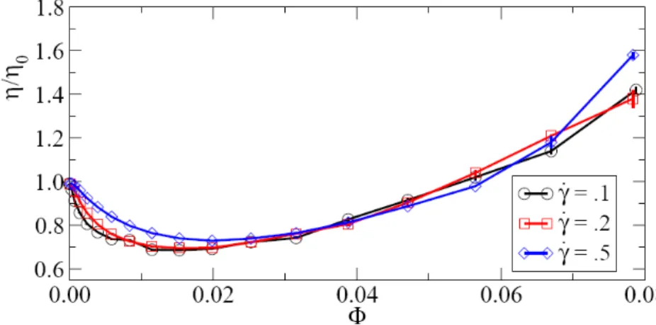
Figure 1.6: Relative Viscosity as function of the volume fraction Φ at different strain rates ˙γ for a "pusher" model. From Ryan et al. (2011).
11
Figure 1.7: (A) Experimental setup of Sokolov and Aranson (2009), using a thin liquid film of bacteria suspension between four movable fibers. (B) Relative viscosity for 6 different concentrations.
bacteria suspension both analytically and numerically (see fig.1.6). They studied the influence of the hydrodynamic interactions on the effective viscosity, showing that this interaction produces an viscosity reduction and, also, that no tumbling is needed to obtain this effect.
From an experimental point of view, there are few studies on viscosity of active suspensions. In 2007, Chen et al. studied nonequilibrium properties of E. Coli bacterial
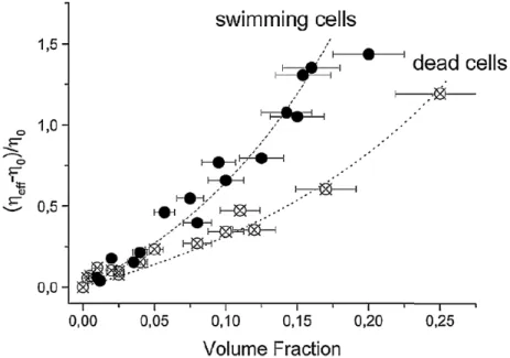
Figure 1.8: Relative viscosity as function of the Chlamydomonas Reinhardtii concentration for a shear rate of 5 s−1. Rafaï et al. (2010).
12
bath through measurements of correlations of passive tracer particles. Sokolov and Aranson in 2009 studied effective viscosity of Bacilus Subtilis ("pusher" type) suspen-sions. The study was performed in a film where a controlled vortex is applied and the viscosity is measured through the relaxation characteristic time (see fig.1.7). They showed a strong reduction of the viscosity (up to 7 times) for concentrations ranging between 1 to 3×10¹⁰Bacteria/cm3). In 2010, Rafaï et al. studied the viscosity varia-tion on Chlamydomonas Reinhardtii algae suspensions. They showed an increase of the viscosity with the volume fraction. This effect was stronger for living algae than for the dead ones (see fig.1.8).
Collective behavior
Moreover, in the case of dense suspension, the presence of living entities offers the possibility to move collectively, organized and synchronized at a mesoscopic level (Koch, 2011). These collective effects can have two origins; either from short range in-teractions and dipolar orientation such as in flocks and herds models (Gregoire, 2004) or, via long range hydrodynamic coupling as in semi-diluted particulate fluids (Sain-tillan, 2007). A primary consequence of this organization will be to yield anomalous statistical behavior either in the spatial distribution of swimmers or in their velocity correlations. These mesoscopic organization properties will have a strong influence on the macroscopic constitutive relations and can be at the origin of complex dy-namical patterns. The situation of long range hydrodynamic coupling is certainly the least studied theoretically, essentially due to the difficulty to solve the full N-body
Figure 1.9: (A) Scanning electron micrograph of the device for the interaction of bacteria with the suitable wall. (B) Uniform distribution after injection. (C) Steady-state distribution after 80 min. (Galadja et al., 2007).
13
hydrodynamic interactions; a question that remains timely also in the case of passive suspensions.
Active density control
It was shown recently that E. Coli bacteria show very singular spatial distributions when they are confined in specific geometries. If the volume is split in two by setting a wall of suitable design, the concentration at both sides of this boundary will be dif-ferent due to the interaction of bacteria with the wall. In 2007 Galajda et al. presented a chamber with a splitting microfabricated wall of funnel-shaped openings that traps alive bacteria (see fig.1.9). Hulme et al. (2008) presented a channel of suitable shape that directs the motion of E. Coli due to their interaction with walls. No external flow is involved and bacteria moves in a very confined system (1.5 µm height) made by PDMS lateral and top walls and a bottom wall made of Agar (see fig.1.10). These
Figure 1.10: Ratchets were design in order to direct the motion of the bacteria. Several trajec-tories are shown after the cell in the left side of the channel (from 1 to 5) and how the cell is reoriented when it gets in in the "wrong side" (from 6 to 10). Bacteria re-concentration after passing by successive ratchets. The arrow indicates the direction in which the ratchet guided cells. (Hulme et al., 2008).
14
results open the possibility to play with the geometrical shape to controlled and sort the population of active swimmers.
In this thesis, the protocoles and large parte of the practical study using E. Coli were defined in close interaction with Dr Annie Rousselet, biologist at the PMMH.
In the first part of the thesis I investigate the Brownian motion of passive trac-ers activated by different active suspension conditions. The Brownian diffusivity was monitored in different environments changing the buoyancy of the suspension as well as the wall confinement. This Part also contains a simple model of the bacte-ria interacting with a wall, developed in collaboration with J. Dunstan and R. Soto from University of Chile. Furthermore we explored a different type of swimmer us-ing synthetic micro-rods in collaboration with Pr Thomas Mallouk from Penn-State University.
The second part includes two experiments on bacteria in a flow. We investigate both: the active viscosity of active suspensions and the anomalous dispersion of a confined bacterial flow. The first topic was addressed in colaboration with Jérémie Gachelin in the framework of his Master’s thesis. From the design by Guillot (2006), we developed, tested and used a viscometer suitable for W wild type E. Coli suspen-sions in the dilute and semi-dilute limits. In Chapter II.2, I conducted experiments in collaboration with Pr Ernesto Altshuler from the University of La Havana at the occa-sion of his sabbatical at the PMMH in 2010-2011. Bacterial suspenocca-sions of E. Coli were transported through an specially designed micro-fluidic channel. The design includes a constriction placed at the middle of the device, called hereafter, the funnel. The in-fluence of geometry and confinement on both the dispersion and transport properties of a bacterial flow, was studied using this simple but archetypal configuration.
Part I
I.1
Methodology and Protocol
I.1.1 Experimental Setup 17
From the perspective of providing a fully consistent treatment of active hydro-dynamics, with important applications in clarifying bacterial transfer in biological micro-vessels, microfluidic devices or the formation of bio-films, a reliable descrip-tion of fluid activity in the vicinity of a solid surface is strongly needed. As described in the introductory chapter for bacteria such as E. Coli, in the presence of a solid boundary due to the head contra-rotation in lubrication interaction with the solid boundary, most trajectories are circle-like and the run time increases significantly. To tackle this open and timely question, I studied the effect of enhanced diffusion pro-duced by a wild type E. Coli on a passive tracer, close to a solid surface. This study follows the pioneering work of Wu and Libchaber (2000), who provide evidence of an activated Brownian motion for bacteria suspensions trapped in a thin film. This is in fact a measurement of the fluid activity. In the experiments presented in this part of my thesis, the activated Brownian motion was monitored in various confined environments, changing the buoyancy (distance to the bottom wall) and exploring another boundary condition (approach of a top surface). In addition, to investigate the influence of a swimming mode significantly different from a biological one, we also compare to the results of an artificial self-propelling system.
I.1.1
Experimental Setup
The setups used in all the experiments presented in this thesis, have several elements in common. Each chapter will be provided with specific setup details, however gen-erally to conduct the observations on the bacterial suspension, I used a Z1 inverted microscope from Zeiss-Observer. Images and videos were captured using a Pixelink PL-A741-E CCD digital camera, connected to and controlled by a computer which stores the images that will be post-processed. The CCD chip has a maximum resolu-tion of 1024×1280 pixels2 and can run at 10 f rames/s full frame. However to gain speed of acquisition, I usually reduced the visualization field to work at 600×800 at a rate of 20 f rames/s.
For the experiments on activated Brownian motion, the principle is to follow the motion of passive particles in a bacterial suspension, in the vicinity of a solid bound-ary. These tracers are Beckman-Coulter latex beads (see Appendix A for details) with a size of either 1 or 2 µm. A 10 µl drop of the following containing the W wild-type E.
I.1.1 Experimental Setup 18
Figure I.1.1: (A) Sketch showing a general view of the chamber used in the experiments. (B) shows a lateral view of the chamber observed on the microscope. For these experiments a 40X objective (Aperture number AN 0.65) was used, given a visualization field of 96×128 µm2. Observation are performed in the center of the drop far away from the drop border.
Coli bacteria (see Archer et al.,2011) and the tracer latex beads, are placed in a trans-parent chamber on the visualization stage of the microscope. A sketch of the chamber is shown in fig. I.1.1. The chamber is made of two cover-slips separated by a typical distance h of 110 µm (achieved by using two cover-slips N◦0 as spacers).
The choice of the ambient medium is always a difficult issue as it may modify strongly the bacteria behaviour in terms of chemotaxis, ambient fluid viscosity or re-sponse to pH. In the literature, several preparation protocols were designed to be able to achieve different goals. For example, for E. Coli, Berg and Brown (1972) defined an specific protocol to study the chemotaxic effects of amino-acids in the bacterial response. A different protocol was chosen by Lowe et al. (1987) as they seeked to change the viscosity of the suspending medium to study the rotation of flagella bundles with Streptococcus. Note that in general, the biological conditions impose a very narrow window of parameters and in practice it is always difficult to conduct experiments that change one parameter at a time as soon as a set of working condi-tions is established. In the present study, to change buoyancy and swimming speed, I will consider two different solutions as a swimming medium: (i) a Minimal Motil-ity Medium (MMA) alone and (ii) a (1 vol/1 vol) mixture of MMA and Percoll (a nanoparticles suspension see Laurent et a.l, 1980) which achieve non-buoyant condi-tions (see Appendix A).
- The use of MMA as swimming solution has several advantages. First, it con-tains a sufficient amount of nutritional elements to preserve the bacteria metabolism (essentially lactose), but cell division is strongly reduced, thus allowing to control density of the bacterial population and limiting the influence of chemotaxis. Second,
I.1.1 Experimental Setup 19
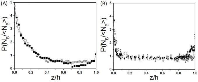
Figure I.1.2: (A) Distribution profile as function of height in buoyancy solution (Mini-mal Motility Medium at pH 7) for two bacterial concentration n (4.5×10⁸bact/ml and 7×10⁸bact/ml) corresponding to optical densities OD 0.7 and 1, respectively. (B) Same exper-iment non-buoyant solution for four bacterial concentration n ranging from 3.8×10⁸bact/ml (OD=0.4) to 7×10⁸bact/ml (OD=1) (mixture of MMA-Percoll at pH 6.9) . z/h=0 and z/h=1 correspond to the bottom and top glass walls of the chamber, respectively.
this medium allows to change the bacteria velocity by modifying the pH of the so-lution, thus acting directly on the molecular proton motor that activates the flagella rotation (see Minamino et al., 2003). A third advantage is that for different values of pH, the MMA solution keeps physical properties similar to water as far a density and viscosity are concerned (See appendix A).
- The MMA-Percoll mixture gives optimal condition to work at different buoyancy. The use of a nanoparticle suspension has a decisive advantage to suppress the risk of a cellular osmotic shock. The bacteria and the latex particles are slightly denser than the MMA solution. Regarding the bacteria density, literature does not provide specific values but it is usually larger than MMA. For the beads, the data-sheet by the manufacturer specifies a value of ρ = 1.027g/ml. In order to reach a density similar of the one of the latex beads I chose to mix in equal proportion these two solutions, obtaining a relative density matching of about 1 % at 25◦C for the tracers. However, contrary to MMA as such, this solution has the disadvantage that pH modifies the mixture viscosity (a factor 2 for pH varying from 6 to 8). For this specific reason, I decided to perform the experiments in quasi isodense conditions at a fixed pH value of 6.9 that provides optimal swimming conditions for the bacteria (for details see
I.1.1 Experimental Setup 20
appendix A).
In all these experiments, special attention was given to avoid the adhesion of latex beads and bacteria on the surface. This was achieved by adding 0.005 % in volume of Polyvinylpyrrolidone (PVP 40 from Sigma Aldrich) to the solution, a protocol used by Berke et al. (2008). Note that glass surfaces were also coated with PVP. Protocol details can also be found in appendix A.
Given this specific preparation protocol, once the chamber is placed under the microscope, a steady distribution of bacteria in the z direction is reached very rapidly. I checked explicitly for the isodense suspension, that in less than 1 minute the bacteria concentration at the center of the chamber reached a steady value. The measurements typically starts a few minutes after the chamber is placed under the microscope. Note that for experiments with MMA alone one has to wait few minutes more in order to let the latex beads sediment. On figures I.1.2.(A) and (B), I display bacteria concentration profiles in the vertical direction for the two types of solutions used (i.e. MMA in (A) and MMA+percoll in (B)) at different mean concentrations.
In the first case (MMA alone), due to buoyancy, there is as accumulation of bacteria at the bottom wall (z/h =0). This is in contrast with the second case (MMA-Percoll), where the bacterial concentration is constant in the center of the chamber and in-creases when it gets close to the walls (within 10 µm (z/h ∼0.1) distance). Note that due to a slight residual density mismatch, one still observes a small sedimentation effect for the MMA-Percoll experiments visualized as an asymmetry in concentration at the wall (see figure I.1.2.(B)). The attraction effect is due to the fact that from the hydrodynamic point of view the surfaces act as traps for the bacterial motion. We discuss this important point in the next section.
Note that in order to monitor the global concentration of bacteria in our prepa-ration procedures, we use a spectrophotometer Hitachi U-2000, which provides the absorption of the suspension at a wavelength of 595 nm. From the optical density (OD) a calibration curve was established to obtain mean bacteria concentrations up to 1.3×10⁹ bact/ml (OD=1.5).
The mean density of bacteria was adjusted to reach densities at the surface that could be described as a “dilute regime" i.e. corresponding to figure I.1.3.(A) (OD <
I.1.1 Experimental Setup 21
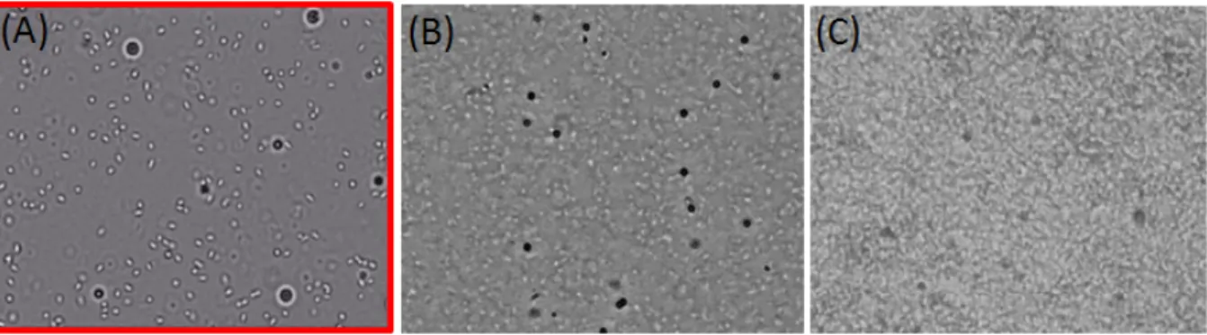
Figure I.1.3: A) Dilute Bacterial suspensions. B) Semi-Dilute Bacterial suspensions C) Concen-trated Bacterial Suspension. Biofilm formation.
1.5). The central figure, I.1.3.(B), could correspond to a semi-dilute regime (1.5 <
OD < 2). At higher concentrations a bio-film would be formed rapidly. The main focus of this thesis is on the first regime.
I.1.1.1
Hydrodynamic trapping at the walls
The accumulation of bacteria like E.Coli (pusher swimmers) at a solid surface was reported and measured quantitatively by Berke et al. (2008). A qualitative explana-tion was given by the same authors, and involves the attractive character of a force dipole in hydrodynamic interaction with its image. Actually this effect should exist in principle but should be very small indeed unless the dipole comes very close to the surface. It is then very likely that in this case, other forces will play an important role such as lubrication forces and also the effects of body and flagellar rotations. All these complications in the hydrodynamic interactions will keep the bacteria very close to the wall. This is why it is possibly preferable to describe the phenomenon like a trapping effect rather than an attraction effect.
From a theoretical and simulation point of view, many authors have been con-cerned about the problem of swimming cells interacting with boundaries. The first numerical work dealing with this subject was presented by Ramia et al. (1993). A bacterium is modelled as a sphere with an helical filament, and the velocity field generated by the swimmer in presence of a wall was computed using a boundary element method. They considered a distribution of punctual forces applied on the surface of the object. The magnitude of the forces was obtained by solving an integral
I.1.1 Experimental Setup 22
Figure I.1.4: Two spheres of different radii connected by a dragless rod, which exerts equal and opposite torques ±τB. Over the T-sphere, a propulsion force f0n is applied by the fluid to mimic the effect of the rotating flagella.
equation for the distribution. The simulation revealed that bacteria swim close to the surface in circles with a radius of the order of the cell length (10µm). The circular motion is clockwise when viewed from the top as observed experimentally. Lauga et al. (2006) approached this problem differently. The same model of swimmers was considered (sphere and helical tail), but the interaction with the wall was taken into account through a resistance matrix which relates the angular and linear velocities with the torques and forces acting on the bacterium. The distance between the swim-mer and the wall is an adjustable parameter of the model and was fixed in the matrix. The effect of the bacterium approaching the wall and the azimuthal stability were not explored. Di Leonardo et al. (2011) studied the interaction between swimming cells (modeled as rod-shaped bodies with an helical flagellum) and a liquid-air inter-face. They considered hydrodynamic interactions of a bacterium with its own mirror image swimming on the opposite side of a perfect-slip boundary. They found that, contrary to solid boundary conditions, the circular rotation is in the other direction (counter-clockwise).
In 2010, Gyrya et al. presented a simplified model of E. Coli introduced by Hernandez-Ortiz et al. in 2005, consisting of two spheres and a punctual force connected by a dragless rod. The interaction between swimmers was investigated.
In collaboration with Rodrigo Soto’s group from the University of Chile and for the master’s thesis of Jocelyn Dunstan, we developed a two sphere E. Coli model interacting with a non-slip surface, inspired by the work of Gyrya et al. (see Fig. I.1.4). Our aim was to investigate the dynamics of swimmers approaching the wall and also
I.1.1 Experimental Setup 23
Figure I.1.5: A) Initial condition for the swimmer: the orientational angle with respect to the surface is α(0), and the position of the center of sphere H is z(0). The geometrical parameters are aH =1µm, aT =0.5µm, L=2µm, and the gap size is set to e=0.01µm. B) Phase diagram of the initial conditions. Three situations are observed: (I) swimming in circles in contact with the wall, (II) swimming parallel to the wall at a finite distance, and (III) swimming away from the wall. The upper left corner is forbidden by the condition that the T sphere must be above the surface. C) Sketch of the three final regimes.
the hydrodynamic possibilities of escapism of the swimmers far from the wall. Both spheres have a different diameter and they are linked by a dragless rod. In figure I.1.4, the model is sketched. The bigger sphere is considered to be the head and the smaller one the tail on which a propulsion force was imposed in order to mimic the effect of flagella. Opposite torques exerted by the rod over the spheres were introduced to consider the axial rotation of the cell. The hydrodynamic forces and torques on each sphere are computed by taking into account the full interaction with the wall surface using the complete resistance matrix. The hydrodynamic interactions between the spheres was computed by superposing the effect that both spheres have on each other. The details of the calculations are presented at the end of the manuscript, in the paper Dunstan et al. (2012) accepted to be published in Physics of fluids.
We investigated for a given geometry of the bacterium, the final trajectories under-taken by the swimmer, by means of two control parameters: the initial distance to the wall z(0) and α(0), the initial angle between the bacterium director and the surface (see fig. I.1.5.A). We chose the model parameters to match the experimental observa-tions of E.Coli swimming. Considering only hydrodynamic interacobserva-tions and an initial condition where the swimmer starts to move with it’s head pointing towards to the surface, we found a family of trajectories for which the swimmer stops its motion
I.1.1 Experimental Setup 24
after reaching the wall.
To remove this singularity, we had to introduce a gap size e (smaller than the bac-terium scale), which cuts off the hydrodynamic forces and would account for the re-ality of surface roughness or any other physical-chemical interaction (like Derjaguin-Landau-Verwey-Overbeek (DLVO) potential) that could overcome at some distance, the hydrodynamic forces. Experiments using the TIRF technique have shown for a Caulobacter Crescentus bacterium, that the minimal distance of approach can be 10 nm (Li et al., 2008). We found three different behaviours, depending on the initial condi-tions. These results are summarized on Fig. I.1.5.(B). If the motion starts with an angle pointing significantly towards the surface, the swimmer will approach the wall until contact with both spheres. Once the system reaches this state, the swimmer starts a circular motion at constant speed and with a radius of curvature in the range of 8-50
µm, depending upon the value used to regularize the resistances (consistently with
experimental data). In the framework of the present model, the swimmer remains in this state forever (domain I on Fig. I.1.5.(B)). A second regime can be reached for intermediate range of height and angle (domain II). In this case it approaches the sur-face without touching it, swimming parallel to it, keeping a gap of approximately half a micron. The trajectory is also circular and the radius is similar, but it swims faster. At last, if the swimmer is initially placed far enough from the wall, and pointing up-wards, it will be able to escape from the surface. Details can be seen in Dunstan et al. (2010 and 2012).
In the previous picture, the dwelling time of a bacterium at a surface when it reaches it is infinite, which makes it a perfect trap. However, it is expected that surface accidents, thermal noise, velocity agitations or the tumbling mechanism can allow the swimmer to exit the region near the wall. In a recent contribution Drescher et al. (2011) investigated in detail this issue from an experimental, a theoretical and a numerical point of views. They measured for E.Coli a dwelling time at a surface that can be as large as a minute. They argued that this dwelling time in this imperfect hydrodynamic trap is indeed sensitive to the rotation diffusion in the azimuthal direction.
As a consequence, in the perspective of developing a reliable hydrodynamic model for bacterial fluids there is a big interest to understand in great details the role of surfaces as boundary conditions and in particular to measure consequences of the
I.1.2 Experimental characterization of bacteria trajectories at the walls 25
hydrodynamic fluctuations caused by autonomous swimmers present at a surface. This is the purpose of the next sections.
I.1.2
Experimental characterization of bacteria
trajecto-ries at the walls
Now I studied the motion of bacteria and passive tracers close to the wall. The fol-lowing sections will describe the procedure used to monitor their motion. I will start presenting the method used to recognize and characterize the bacterial population in terms of motion at the surface. Then I will continue with the explanation of the procedure used to compute the diffusion of passive tracers.
I.1.2.1
Bacteria Detection
For all experiments described in the following section, I used a 40X magnification objective (NA =0.65) using a direct illumination. I positioned the focal plane at a constant and reproducible height of about 2.5±0.5 µm above the surface to identify the bacteria below the focal plane as a bright spot.
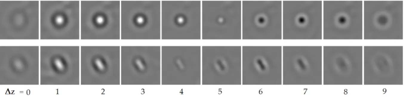
Figure I.1.6 displays a sequence of images for two kinds of bacteria stuck at the solid surface, taken every 1 µm (for the microscope Z-stage position). Note that in
Figure I.1.6: Two different bacterium stuck to the surface are shown at different height from the bacteria focal plane. When a bacterium is in focus, a dark body with a halo appears in the image. The first image (left one) was taken far above the focal plane. Each images was taken with a∆z equal to 1 µm.
I.1.2 Experimental characterization of bacteria trajectories at the walls 26
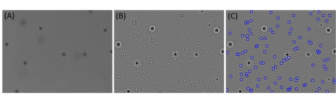
Figure I.1.7: (A) Unprocessed image of E. Coli solution containing passive tracers close to the bottom surface. Bacteria appear as a bright object and it is difficult to distinguish. (B) Same image after the analysis processing. It can be notice that the contrast has been increased. (C) The blue circles represent the position of the bacteria, drawing using a 10 pixels diameter circle.
order to get the actual position in the fluid, one has to multiply by the index of refraction n ≈ 1.3. We see indeed that the bacteria below the focal plane display a bright core surrounded by a dark ring. I always managed to identify a bacterium close to the surface (there is a small fraction of them stuck on the glass slide) and adjust the vertical position in an intermediate position that corresponding typically to ∆z =2 on fig. I.1.6. Note also that we have then an observation field (in the fluid) of approximately 5 µm. This value will be important to calculate the concentration close to the surface.
Interestingly, note that on this picture I displayed two cells with different shapes. They actually correspond to cells at different stages of the division cycle. The top one is quite circular and is a bacterium emerging from the fission. We call it a “baby cell" and in the literature it is currently referred as a 1N bacterium. The one on the second line is more elongated and it corresponds to a bacterium at a later stage that has duplicated its DNA, it is called a 2N bacterium.
To identify the bacteria, videos of 20 seconds were recorded at 20 frames per sec-ond (sequences of 400 images). Each image stored in Tiff format, was post-processed using a macro program developed on ImageJ. Figure I.1.7.(A) shows for a typical ex-periment, an image of the bacteria and the particles at the bottom surface. It can be noticed that bacteria and latex beads appear in the image as bright and dark bodies, respectively. The main idea of the image processing is to distinguish automatically bacteria from passive tracers and to determine their positions. Generally speaking,
I.1.2 Experimental characterization of bacteria trajectories at the walls 27
each image was processed using 3 kinds of filters (Fourier low pass band, Gaus-sian and Unsharp Mask ) and then the maximal levels of gray were searched using quadratic fits in order to find the particle positions. For details on how images are processed, refer to appendix B. Figure I.1.7.(B) shows the corresponding post pro-cessed image, after the filtering. Fig. I.1.7.(C) illustrates the bacteria detected by the macro program.
I.1.2.2
Bacteria Tracking and Trajectory Analysis
Once the particles positions are found, the individual trajectories are reconstructed using a tracking program developed in C++. This program was developed by Thierry Darnige at PMMH lab (see Appendix B). This program provides a collection of tracks starting when a bacterium is detected until it disappears. Note that a problem may occur when eventually two bacteria come in close contact, the tracking program can either confuse the individuals of loose track. This is an issue which may create sys-tematic detection problems of the paths at higher density. We operated in densities
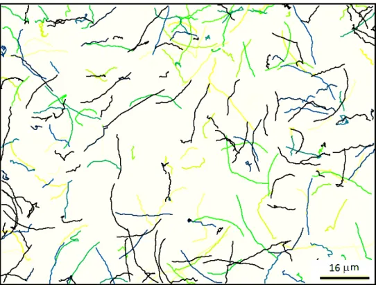
Figure I.1.8: Different bacterial trajectories. Each color represents a different bacterium and the duration of the trajectories displayed is 1.5 seconds.
I.1.2 Experimental characterization of bacteria trajectories at the walls 28
Figure I.1.9: Definition of θ that will give the mean persistence angle | < θ > | for the
trajectory.
low enough so that the track persistence is high and the bacteria can still be followed for more than 10 s.
For the wild-type bacteria, we actually noticed that two different kinds of motion can be observed close to the wall. The first one corresponds to smooth trajectories such as circles or lines. The second type looks more like a random motion (different from a run and tumble motion usually found in the literature (Fig. I.1.8)). This is why I developed a program suited to clearly distinguish these two types of “populations" which may have a different influence on the fluid activity. Actually, I do not exactly know if the diffusive bacteria are with broken flagella or temporally inactive but for a given preparation, I was usually left with a ratio of them which was for a large part unpredictable (in spite of many attempts to do so). For each experiment, the images were processed to extract all the possible bacteria tracks. From each trajectory, I measured two structural parameters: the mean persistence angle (| < θ > |) of the
walk and the Nc ratio representing the track "compactness".
- The persistence angle is defined based upon the positions of a bacterium taken at three successive images (see fig. I.1.9). The average is performed over all the steps
I.1.2 Experimental characterization of bacteria trajectories at the walls 29
in the trajectory. Note as an illustration that for a random walk and a linear trajectory one would obtain respectively the values:
|<θ>|→π/2 (random walk)
|<θ>|→0 (straight line)
- The Nc ratio represents the ratio between the maximal exploration distance of the track L (see figure I.1.10 for an illustration) and the total length of the line. Its definition is:
Nc = L/T
<dr >/δt (I.1.1)
were L is maximal exploration distance of the track, T is the trajectory duration,
< dr > is the mean absolute value of the displacement and δt, the acquisition time (1/20 s).
With this definition when the trajectory is a straight line NC tends to 1. In this case the value L/T and < dr > /dt can be interpreted as the mean and the instanta-neous velocity, respectively. For a diffusive process NC tends to 0 for large trajectory durations.
Therefore, each track is associated with these two numbers (Nc, <θ >), defining a
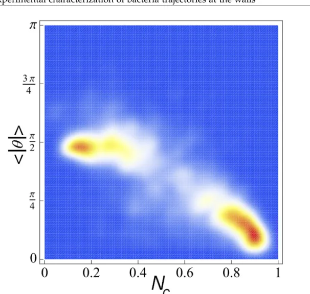
point in a 2D space of parameters. On figure I.1.11, I display the map of the probability density obtained for 1000 bacterial tracks extracted from 4 experiments at the same mean concentration and obtained in similar conditions. The color map goes from blue (vanishing probability) to red (maximum probability). The four experiments were chosen as they seemed to show different behaviour in terms of the type of motion that bacteria may undergo. And indeed, one observes two distinct clusters in the (Nc, < θ >) space, that can be identified as a clear separation between what we
will call from now : "active swimmers" and "random swimmers". Since this method does not predict the swimming behaviour for short or interrupted trajectories, tracks shorter than 10 steps were systematically discarded. In practice I chose to separate the behaviour by the line represented on the figure (line of equation : y=2.44x).
I.1.2 Experimental characterization of bacteria trajectories at the walls 30
Figure I.1.11: Density probability of the observed bacterial tracks in the (Nc,|<θ>|) space. The color map goes from blue for vanishing probability to red for high probability. Two clusters are identified, centred at (0.9, 0.3) and (0.17; /2), corresponding, respectively, to the active and random swimmers.
Therefore, now we are able to classify the motions into two major groups and to define at each time, a number of active swimmers NA(t). The mean fraction of active bacteria φA is then defined as the mean number of active bacteria (time averaged) divided by the mean number of bacteria (time averaged). Fig. I.1.12 shows two examples of bacterial populations that differs in φAbut have about the same bacterial concentration. Active trajectories are colored in red and the random ones, in blue.
I.1.2 Experimental characterization of bacteria trajectories at the walls 31
Figure I.1.12: Identification of the swimmer populations by tracking active swimmers (red tracks) and random swimmers (blue tracks), φA is the corresponding fraction of active swim-mers.
I.1.2 Experimental characterization of bacteria trajectories at the walls 32
Figure I.1.13: Mean Square Displacement computed with the trajectories of bacteria that are classified as random swimmers in isodense conditions. Thick black line corresponds to the average curve. 4DR represents the slope of the curve, and from the linear fitting, DR = 0.34µm/s.
I.1.2.3
Population Motility Characterization
For a specific experiment, once the populations are classified, their motion on the surface can be characterized separately.
Random Swimmers
The random motion can be characterized by the mean square displacement MSD calculated as a function of the time lag τ, as illustrated in fig. I.1.13. The slope is 4DR, where DR is the diffusion coefficient. In the case of the so called random bacteria, it can be noted that not all the analysed trajectories have a diffusive behaviour (i. e. no linear relation between MSD and the time lag), but the average of all the curves has (thick black line in fig. I.1.13). From here we can estimate a mean value of DR = 0.34µm/s. Furthermore, for an experiment, the mean value DR can be computed also by averaging all the tracks. For the experiment presented in fig I.1.13), this calculation
I.1.2 Experimental characterization of bacteria trajectories at the walls 33
Figure I.1.14: Bacterial diffusion distribution for different φA. DR represents the mean diffu-sion of the random population. DR represents the mean diffusion of the random population. Experiments shown in this graph were performed in isodense condition. Half heigth width range from 0.6 to 0.62
gives a value of DR = 0.32µm/s. On Fig.I.1.14, I display the normalized distribution for different fractions of active bacteria and different concentrations. It seems that the distribution shape does not vary too much. I will discuss the variations of the mean diffusivity DR in the next chapter.
Active Swimmers
In the case of active bacteria, for each track I defined the mean track velocity V, which is the trajectory length divided by the total time. The mean velocity VA is the average of this velocity over all the detected tracks. Note that I also checked an alternative definition of the mean velocity by weighting the mean by the track length but it did not change anything. On Fig. I.1.15, I displayed the normalized velocity distribution for different values of the active φAat two different bacteria densities, for the isodense suspension. These distributions do not seem to vary very much.
I.1.2 Experimental characterization of bacteria trajectories at the walls 34
Figure I.1.15: Velocity distribution for different experiments in isodense condition. Each sym-bol represents different active fractions φA. VArepresents the mean velocity of the active popu-lation. Empty and filled symbols distinguish between a mean number of bacteria<N >=100 and< N >=200 in the visualization field, respectively. Half heigth width range from 0.90 to 0.95
On Fig I.1.16, I display the velocities of active swimmers (VA) as a function of the active fraction (φA), for different experiments. Several synchronization protocols were tested in order to select bacteria at different stages of the cell cycle, which could display different swimming characteristics. We were able to produce “baby-bacteria” populations (1N short cells, 1,12 µm long) with a fraction φA much larger than the one expected for more mature bacteria populations (2N long cells, 2,5 µm long) (see fig. I.1.6). We took advantage of this difference to analyze the influence a fraction of active swimmers φAon the mean velocity VA. Each color stands for a same population of E. Coli. The number of bacteria in the visualization field is distinguished, by the labels 1 and 2 corresponding respectively to < N >=100 and < N >=200. On this figure we did not see any clear dependency of the mean velocity when doubling the concentration and changing the active fraction. These results in conjunction with the invariant distribution shape of Fig. I.1.15 are in favor of a low density limit where collective effects play a marginal role.
I.1.2 Experimental characterization of bacteria trajectories at the walls 35
Figure I.1.16: Relation between the active swimmer’s mean velocity VA and φA. Colors rep-resent 6 independent experiments with E. coli: 1N cells (brown, red, and green), mixture of 1N and 2N cells (black), and 2N cells (pink, blue). Labels (1) and (2) are for< N>=100 and < N>=200 cells in the observation field, respectively.
As mentioned before, several authors have observed that bacteria move in circular trajectories when they swim close to a solid surface( DiLuzio et al., 2005; and Lauga et al., 2006) and the dispersion in the radii had been related with the cell dimension. Following these observations, I was interested in the characterization of this circular motion using "baby cell" experiments, where the aspect ratios of the cells are in an narrow windows close to 1. The analysis of each trajectory was performed by circular fitting using the least square method to compute the radius. Fig. I.1.17 shows a trajectory example close to the wall and the circle obtained through the fit.
This fitting procedure is performed for all the trajectories of the experiment and from here, the distribution of radii can be computed. Fig. I.1.18 presents the normal-ized distribution of radii, measured in our setup for populations of different numbers of bacteria in the visualization field and high φA. In the same way, the normalized distributions do not seem to vary much with the concentration variations.
I.1.2 Experimental characterization of bacteria trajectories at the walls 36
Figure I.1.17: Example of a circular trajectory fitted with a circle of 31.2 pixel radius. Scale: 1 pixel=0.16 µm.
Figure I.1.18: Four normalized distributions are displayed, corresponding to experiments with constant active fraction at different bacterial concentration in isodense conditions. Each dis-tributions was obtained by fitting all the trajectories in the experiment with circles.
I.1.3 Motion of Passive Tracers 37
Figure I.1.19: Representation of the pair (< R >, VA) for the different experiment presented in the previous graph.
fig. I.1.19) in spite of a significant data scatter, we observe a relation that seems to be increasing. Note that this relation might not be linear as witnessed by the effective power law presented as guide to the eyes. Importantly, we used in this experiment essentially "baby runner cells" within a synchronization protocol producing bacteria of about the same size and shape. We argue that this relation could be a consequence of a distribution of approaches to the surface and not a consequence of the variability in shape as argued by other authors Lauga et al., 2006.
I.1.3
Motion of Passive Tracers
As noticed previously, the latex tracers always appear as dark objects (see Fig. I.1.20). This facilitates their detection when they are close to the surface. To follow them, sequences of 300 images are registered at 1 frame per second (representing a total observation time of 5 minutes). Following a similar image analysis and a tracking procedure as the one described for the bacterial motion, their trajectories are identified (See Appendix B).
I.1.3 Motion of Passive Tracers 38
Figure I.1.20: A). Unprocessed image of E. Coli solution containing passive tracers close to the bottom of the chamber. The passive tracers or beads appear as dark spots and E. Coli as bright objects. (B). Same image after processing. Beads become bright and contrast with the background. (C). The blue circles for visualization of beads position, using a circle of 20 pixels diameter centered in the position detected by the macro, were drawn.
Figure I.1.20.(A) shows the original image. This image is processed by the macro, resulting in an inverted image where beads appear as bright objects (Fig. I.1.20.(B)). The same program recognizes the local maximal intensity, then the positions of the beads are identified (Fig. I.1.20.(C)).
After the beads trajectories are obtained (Fig. I.1.21), the mean square displace-ment (MSD) is calculated for each particle as a function of the time lag τ. For each trajectory of the tracer i, the MSD for a time lag τ , is computed as:
I.1.3 Motion of Passive Tracers 39
Figure I.1.22: Means Square Displacement (MSD) of a passive particle for an observation time of 20 seconds. Left-top inset: same quantity as a function of time smaller than 1 second. Right-bottom inset: illustration of a bead moving close to the wall.
<∆r2(τ) >i=< [~ri(τ+t)−~ri(t)]2>τ (I.1.2) where~ri represents the position of the i-th particle. The average is taken over time t. Figure I.1.22 shows an example of the MSD (<∆r2(
τ) >) as a function of the time lag
(error bars represent standard deviations) for one particle. We see a linear relation-ship, probing a diffusive motion, the slope being four times the diffusion constant:
<∆r2(τ) >=4DPτ (I.1.3)
In the superior inset, times smaller than 1 second are explored. As we still see a linear relationship, it means that we have reached the diffusive limit for time larger than 0.1. Note that for bacteria trapped in a film, Wu and Libchaber (2000) pointed out an anomalous diffusion which could be observed for times shorter than 1 second actually it does not seem to happen in our situation. In any case, in all the following
I.1.3 Motion of Passive Tracers 40
Figure I.1.23: Mean square displacement for passive particles corresponding to one experi-ment. The number of beads varies from one experiment to other (from 6 to 12).
measurements we used a time resolution of 1 s and 5 minutes measurements. The picture in the right-bottom illustrates a bead trajectory close to the wall.
For each experiment, 6 to 12 beads were tracked and trajectories were obtained. Fig. I.1.23 shows the MSD’s obtained for one experiment in which 6 tracers were tracked. The error bars represent the standard deviation of the MSD computed at the corresponding time. We see that we have some dispersion of the diffusion constant. We define the mean diffusion constant by averaging the data points for all beads at a given time-lag and fit the slope by a linear relation. The error bar on the mean diffusion coefficient is computed using the standard deviation from the fit.
In the previously presented case, the trajectories of the tracers did not display any mean drift . This is generally the case, however some times, we noticed the presence of a net flux on the beads (typically few tenths of micron/s, see in fig. I.1.24)). We do not know exactly the reasons for this. It could be a flux of liquid caused by evaporation. However, it could be another effect caused by the activity of bacteria. In any case, we verified that during the measurements the concentration in bacteria did not change significantly. We developed several post-processing procedures to remove these drifts. The data points on mean diffusion extracted by any of these methods were consistent with the other data points when no drift is observed (see I.1.25). The
I.1.3 Motion of Passive Tracers 41
6 different methods described in the following:
Method 1: Here each MSD curve is fit with a linear function like the equation
I.1.3, where the slope of the fitting represents the factor 4D. This method can predict a wrong value if there is a residual drift in the experiment. In case this happens a second method is proposed in order to correct this problem.
Method 2: In this procedure, the fitting function has the form:
<∆r2(τ) >=4Dτ+Vd2t2 (I.1.4)
where Vd represents the eventual drift. The linear term correspond to the diffusive ones and the quadratic term the convective one.
Method 3: here the derivation of MSD is performed and the diffusion term can be obtained from the independent term if we fit the curve with a linear function.
Method 4: Until this stage the determination of the diffusivity uses the MSD after tracking. Here the correction is performed before the computation of the mean square displacement. Each coordinate (x and y) is adjusted by subtracting the convective part.
Figure I.1.24: Passive Tracer trajectories under a drift during 5 min of experiment. The arrow, represents the direction of the flow.
I.1.3 Motion of Passive Tracers 42
Figure I.1.25: Passive Tracer Diffusivity computed using the six different methods described in the text.
So the x or y displacement is fitted by a linear function and then the drift is eliminated. Then the MSD is computed and a procedure similar to method 1 is followed.
Method 5: Here, the same procedure as method 3 is applied but in this case the MSD calculated in the previous method is differentiated and the diffusion is calcu-lated.
Method 6: So far, one particle displacement was taken into account. In this
method, an inter-particles correlation is used to compute the mean square displace-ment. Two particles MSD calculation is computed following the equation:
<∆r2(τ) >ij=< [~rj(τ+t)−~ri(τ+t)]− [~rj(t)−~ri(t)]2 >τ (I.1.5) where~rj and~ri represent the position of the particle i and j, respectively. This defini-tion follows the one presented by Cheung et al (1996).
Fig. I.1.25 shows the results obtained from the different methods for one experi-ment. It can be noted that all the methods give similar values, and that one and two particles MSD have a particularly good agreement.