Algebraic Domain Decomposition Methods for Darcy flow in heterogeneous media

HAL Id: tel-00550728

https://tel.archives-ouvertes.fr/tel-00550728

HAL is a multi-disciplinary open access

archive for the deposit and dissemination of sci-entific research documents, whether they are pub-lished or not. The documents may come from teaching and research institutions in France or abroad, or from public or private research centers.

L’archive ouverte pluridisciplinaire HAL, est destinée au dépôt et à la diffusion de documents scientifiques de niveau recherche, publiés ou non, émanant des établissements d’enseignement et de recherche français ou étrangers, des laboratoires publics ou privés.

flow in heterogeneous media

Mikolaj Szydlarski

To cite this version:

Mikolaj Szydlarski. Algebraic Domain Decomposition Methods for Darcy flow in heterogeneous media. Mathematics [math]. Université Pierre et Marie Curie - Paris VI, 2010. English. �tel-00550728�

DE L’UNIVERSITE PIERRE ET MARIE CURIE

É

COLE

D

OCTORALE DE

S

CIENCES

M

ATHÉMATIQUES

DE

P

ARIS

C

ENTRE

Spécialité

M

ATHÉMATIQUES APPLIQUÉES

Présentée par

M. Mikołaj S

ZYDLARSKI

Pour obtenir le grade de

DOCTEUR

DE L

’UNIVERSITÉ PIERRE ET MARIE CURIE

Sujet de la thèse:

A

LGEBRAIC

D

OMAIN

D

ECOMPOSITION

M

ETHODS

FOR

D

ARCY FLOW IN HETEROGENEOUS MEDIA

Soutenue le 5 Novembre 2010 devant le jury composé de:

Président: M. Frédéric HECHT Laboratoire J.L. Lions (UPMC)

Rapporteur: M. Bernard PHILIPPE INRIA (Rennes)

Rapporteur: M. Luc GIRAUD INRIA (Bordeaux)

Directeur de thèse: M. Frédéric NATAF Laboratoire J.L. Lions (UPMC) M. Roland MASSON IFP Energies nouvelles

be desired cannot be compared to it.”

THEBOOK OFPROVERBS8:10-11

This thesis arose in part out of three years of research that has been done since I came to France. By that time, I have worked with a number of people whose contribution in assorted ways to the research and the making of the thesis deserved special mention. It is a pleasure to convey my gratitude to them all in my humble acknowledgment.

In the first place I would like to record my gratitude to Fédéric Nataf for his supervision, advice, and guidance as well as giving me extraordinary experiences through out the work. Above all and the most needed, he provided me unflinching encouragement and support in various ways. His scientist intuition and wisdom inspire and enrich my growth as a student, a researcher and a scientist want to be. I am indebted to him more than he knows.

Many thanks go in particular to Pascal Havé and Roland Masson. I am much indebted to Pascal for his valuable advice in science discussion, supervision in programming and fur-thermore, using his precious times to read this thesis and gave his critical comments about it. I have also benefited by supervision and guidance from Roland who kindly grants me his time for answering of my questions about the Black Oil model and porous media flow simulations.

I gratefully thank Bernard Philippe and Luc Giraud for their constructive comments on this thesis. I am thankful that in the midst of all their activity, they accepted to be members of the reading committee.

I would also acknowledge Thomas Guignon, whom I would like to thank for taught me how to work with IFP format for storage a sparse matrices originating from the real simula-tions of the porous media flow. It was a pleasure to work with an exceptionally experienced scientist like him.

Collective and individual acknowledgments are also owed to my colleagues at IFP whose present somehow perpetually refreshed, helpful, and memorable. Many thanks go in par-ticular to Carole Widmer, Nataliya Metla, Eugenio Echague, Ivan Kapyrin, Gopalkrishnan Parameswaran, Riccardo Ceccarelli, Safwat Hamad, Hassan Fahs, Florian Haeberlein and Hoel Langouet for giving me such a pleasant time when working together with them since I knew them. Special thanks to Daniele Di Pietro for the coffee break meetings and dry hu-mour about scientist’s life. I also convey special acknowledgement to Sylvie Pegaz, Sylvie Wolf and Léo Agélas for being such good neighbours in the office, who always ready to lend me a hand. I would like also thank to Tao Zhao from LJLL for his generous help in perform-ing a number of numerical experiments which results, thanks to his help some death-lines weren’t so scary.

I was extraordinarily fortunate in having Chiara Simeoni as my master degree supervisor at the University of L’Aquila . I could never have embarked and started all of this without her prior teachings and wise advices. Thank you.

Where would I be without my family ? My parents deserve special mention for their in-separable support and prayers. My Father, Marcin Szydlarski, in the first place is the person who put the fundament my learning character, showing me the joy of intellectual pursuit ever since I was a child. My Mother, Danuta, is the one who sincerely raised me with her

Introduction 12

Definition of problem . . . 12

Future of reservoir simulations . . . 13

Objective . . . 14

Context of work . . . 14

Plan of report . . . 14

1 State of Art 18 1.1 Original Schwarz Methods . . . 19

1.1.1 Discrete Schwarz Methods . . . 20

1.1.2 Drawbacks of original Schwarz methods . . . 23

1.2 Optimal Interface Condition . . . 24

1.3 Optimised Schwarz Method . . . 26

1.3.1 Optimal Algebraic Interface Conditions . . . 26

1.3.2 Patch Method . . . 28

1.4 Two-level domain decomposition method . . . 30

1.5 Discussion . . . 32

2 ADDMlib : Parallel Algebraic DDM Library 34 2.1 Interface for Domain Decomposition and Communication . . . 35

2.1.1 Distributed Memory Architectures . . . 35

Multi-core Strategies . . . 36

2.1.2 Data Distribution in ADDMlib . . . . 38

2.2 Linear Algebra . . . 39

2.2.1 Vector (DDMVector) . . . 40

2.2.2 Matrix (DDMOeprator) . . . 40

Structure and Sparse Storage Formats . . . 41

Matrix-Vector Product . . . 43

2.2.3 Preconditioner . . . 43

ADDM Preconditioning . . . 44

2.3.1 The two domain case . . . 46

2.3.2 Implementation . . . 47

2.3.3 Numerical experiments . . . 49

2.4 Partitioning with weights . . . 50

2.4.1 Implementation . . . 52

2.4.2 Numerical Experiments . . . 53

2.5 Modified Schwarz Method (MSM) . . . 57

2.5.1 The two sub-domains . . . 57

2.5.2 The three sub-domains case . . . 57

2.5.3 Implementation . . . 59

2.6 Sparse Patch Method . . . 60

Patch parameters . . . 60

Patch connectivity strategy . . . 62

2.6.1 Parallel implementation . . . 63

2.6.2 Numerical Experiments . . . 63

3 Enhanced Diagonal Optimal Interface Conditions 66 3.1 Sparse approximation of optimal conditions . . . 66

3.1.1 General case for arbitrary domain decomposition . . . 69

3.1.2 Second orderβ e 1ce1c operator . . . 71

3.2 Retrieving harmonic vector from solving system . . . 72

Right preconditioned system . . . 73

Retrieving approximate eigenvector from GMRES solver . . . 74

3.3 Parallel implementation . . . 75 3.3.1 Implementation ofβ operators . . . 75 Approximated eigenvector . . . 75 Fillingβ operators . . . 76 3.3.2 Computing Sed oi c e ΓIeΓI . . . 76 3.4 Numerical results . . . 78

3.4.1 EDOIC and quality of eigenvector approximation . . . 79

3.4.2 EDOIC versus number of subdomains . . . . 80

4 Two level method 84 4.1 Abstract Preconditioner . . . 84

4.2 The Coarse Grid Space Construction . . . 86

4.3 Parallel implementation . . . 87

4.3.1 Matrix-vector product for compose operatorAe?. . . 88

4.3.2 Matrix-vector product for preconditionerMe−1? . . . 88

4.3.3 Coarse grid correction -Ξ . . . 89

Operation [DDMOperator][SVC] = [SVC] . . . 89

Operation [SVC]T[DDMVector] = [v ∈ RnVN_{] . . . . 90}

Operation [SVC][v ∈ RnVN_{] = [DDMVector] . . . . 91}

4.4 Numerical results . . . 93

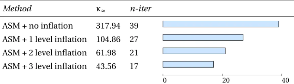
4.4.1 Successive and Adaptive two-level preconditioner . . . 94

4.4.2 How to read plots . . . 94

4.4.3 Two-level preconditioner versus quality of eigenvectors approximation and size of coarse space . . . 94

4.4.4 Two-level preconditioner versus number of subdomains . . . . 96

4.4.5 Two-level preconditioner with Sparse Patch . . . 98

2D Case . . . 98

3D Case . . . 99

4.4.6 Reservoir simulations - experiment with Black Oil model . . . 101

5 Numerical Experiments 116 5.1 3D Laplace problem . . . 116

5.1.1 Setup of the Experiment 5.1 . . . 116

High Performance tests . . . 118

5.2 Algebraic Multi Grid method as a sub-solver in ADDM . . . 128

5.2.1 Setup of the Experiment 5.2 . . . 128

5.3 Real test cases . . . 132

5.3.1 IFP Matrix Collection - pressure block only . . . 132

5.4 IFP Matrix Collection - system of equations . . . 145

5.5 Black-Oil Simulation: series of linear systems from Newton algorithm. . . 153

5.5.1 Black-Oil - 60 × 60 × 32 . . . 154

5.5.2 Black-Oil - 120 × 120 × 64 . . . 156

Definition of problem

Porous media flow simulations lead to the solution of complex non linear systems of coupled Partial Differential Equations (PDEs) accounting for the mass conservation of each component and the multiphase Darcy law. These PDEs are discretized using a cell-centered finite volume scheme and a fully implicit Euler integration in time in order to allow for large time steps. After Newton type linearization, one ends up with the solution of a linear sys-tem at each Newton iteration which all together represents up to 90 percents of the total simulation elapsed time. The linear systems couple an elliptic (or parabolic) unknown, the pressure, and hyperbolic (or degenerate parabolic) unknowns, the volume or molar frac-tions. They are non symmetric, and ill-conditioned in particular due to the elliptic part of the system, and the strong heterogeneities and anisotropy of the media. Their solution by an iterative Krylov method such as GMRES or BiCGStab requires the construction of an efficient preconditioner which should be scalable with respect to the heterogeneities, anisotropies of the media, the mesh size and the number of processors, and should cope with the coupling of the elliptic and hyperbolic unknowns.

In practice, a good preconditioner must satisfy many constraints. It must be inexpensive to compute and to apply in terms of both computational time and memory storage. Because we are interested in parallel applications, the construction and application of the precondi-tioner of the system should also be parallelizable and scalable. That is the preconditioned iterations should converge rapidly, and the performance should not be degraded when the number of processors increases. There are two classes of preconditioners, one is to design specialised algorithms that are close to optimal for a narrow type of problems, whereas the second is a general-purpose algebraic method. But this kind of preconditioning require a complete knowledge of the problem which may not always be feasible. Furthermore, these problem specific approaches are generally very sensitive to the details of the problem, and even small changes in the problem parameters can penalize the efficiency of the solver. On the other hand, the algebraic methods use only information contained in the coefficient of the matrices. These techniques achieve reasonable efficiency on a wide range of problems. In general, they are easy to apply and are well suited for irregular problems. Furthermore, one important aspect of such approaches is that they can be adapted and tuned to exploit

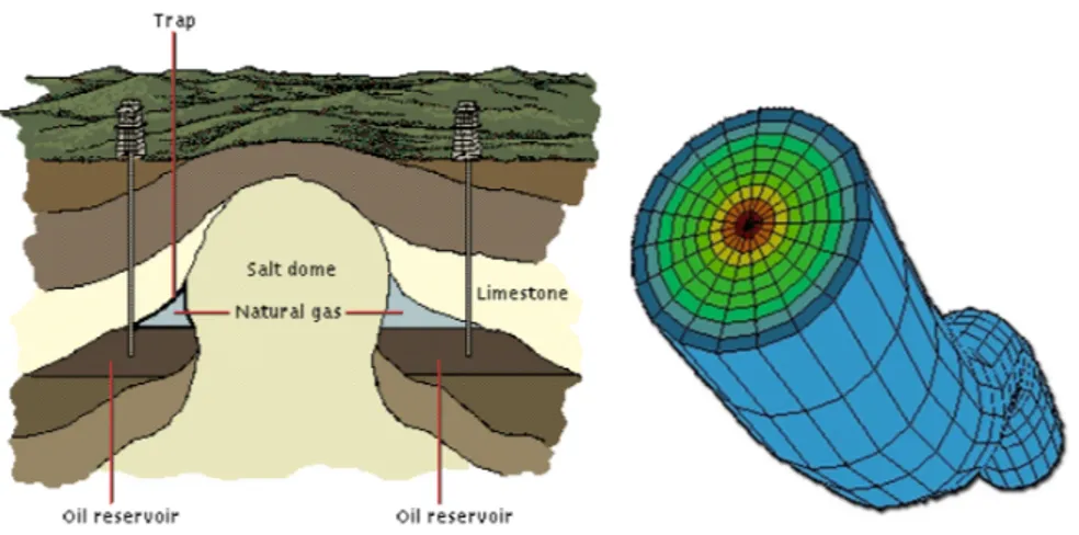
Figure 1: Example of oil reservoir and mesh of complex well

specific applications.

The current IFP solution is based on Algebraic MultiGrid preconditioners (AMG) for the pressure block combined with an incomplete ILU(0) factorisation of the full system. This so called combinative-AMG preconditioner is the most serious candidate for the new genera-tion of reservoir simulators for its very good scalability properties with respect to the mesh size and the heterogeneities.

Nevertheless, this method still exhibits some problems of robustness when the linear sys-tem is too far from the algebraic multigrid paradigm (e.g. for strongly non diagonally dom-inant wells equations or for multipoint flux approximations or non linear closure laws lead-ing to strongly positive off diagonal terms, or for convection dominated equations). Domain Decomposition Methods (DDM) are an alternative solution that could solve the above dif-ficulties in terms of robustness and parallel efficiency on distributed architectures. These methods are naturally adapted to parallel computations and are more robust in particular when the subdomain problems are solved by a direct sparse solver. They also extend to cou-pled system of PDEs and enable to treat in the same framework the coupling of different type of models like wells equations or conductive faults.

Future of reservoir simulations

Continuously increasing demand for accurate results from reservoir simulations indicate usage of more dense and complex meshes along with advance numerical schemes which can deal with them. For example in current IFP models we have only one equation per well. However a new approach is developing in which a well has a complex modelling and refined mesh (see figure 1). In this context domain decomposition is not only an alternative but it becomes the natural choice for separating of model of flow around well and far from it.

Those future plans are another motivation for studying domain decomposition methods for multiphase, compositional porous media flow simulations.

Figure 2: Example mesh of reservoir with complex wells (horizontal and vertical)

Objective

The objective of this PhD is to study and implement algebraic domain decomposition methods as a preconditioner of a Krylov iterative solver. This preconditioner could apply either on the full system or on the pressure “elliptic” block only as the second step of a com-binative preconditioner. Therefore the main difficulties to be studied are the algebraic con-struction of interface conditions between the subdomains, the algebraic concon-struction of a coarse grid, and the partitioning and load balancing within a distributed data structure im-plementation.

Context of work

This work is performed in the framework of convention industrielle de formation par la recherche (CIFRE) under the dual responsibility of Pierre and Marie Curie University (Paris VI) and IFP Energies nouvelles (IFP New Energy)1. Academic side is carried out by Ecole Doctorale de Sciences Mathématiques de Paris Centre on-site Départament Mathématiques Appliquées et le Laboratoire Jacques-Louis Lions. From industrial point of view this thesis is a part of research project of IFP at department of Informatics and Applied Mathematics.

Plan of report

In chapter 1, we give an overview on the existing works on the two main ingredients of the domain decomposition methods: the interface conditions between the subdomains and the coarse grid corrections. As for the interface conditions, since the seminal paper by P.L. Lions [39], there has been many works on how to design efficient interface conditions. The prob-lem can be considered at the continuous level and then discretized (see e.g. [19,28,44]). This

1. In June 2010 IFP (French Institute of Oil) changed name into IFP Energies nouvelles in order to more closely reflects IFP’s objectives and the very nature of its research, with their increasing focus on new energy technologies.

approach, based on the use of the Fourier transform, is limited to smooth coefficients. In this chapter we focus on a method that works directly at the discrete level: the patch method [40]. As for the coarse grid correction, we explain that once the coarse space is chosen, the way to build the coarse grid correction is readily available from the papers by Nabben-Vuik and coauthors [57].

In chapter 2, we present the main features of the library that was developed in order to implement various existing methods and test new ideas. The library is carefully designed in C++ and MPI with a convenient parallel matrix storage that eases the test of new algo-rithms. Our data structure is very close to the one recently and independently proposed in [11]. Otherwise, the library uses as much as possible existing libraries (e.g. Metis and Scotch for partitioning, SuperLU, Hypre and PETSC for the sequential linear solvers). We report ex-periments made with this library testing existing domain decomposition methods: Schwarz methods with overlapping decompositions, partitioning with weights for taking into account anisotropy and discontinuities in an algebraic multigrid fashion, modified Schwarz method with interface conditions including the patch method [40]. The library will be used in the next chapters to test new methods in domain decomposition methods.

Chapter 3 introduces a new algebraic way to build interface conditions. It is shown in Lemma 3.1 that if the original matrix is symmetric positive definite (SPD), the local subprob-lems with the algebraic interface conditions will still be SPD. This construction depends on a parameter β (typically a diagonal matrix). In the two subdomain case, for a given har-monic vector in the subdomain, it is possible to build the interface condition such as to “kill” the error on this vector. This vector is chosen by computing Ritz eigenvectors from the Krylov space. In this respect, the method is adaptive and is very efficient for the two or three-subdomain case. But when there are many subdomains, numerical tests show that the method does not bring a benefit and it is thus limited to the two subdomain case.

This motivates chapter 4 where an adaptive coarse grid correction is introduced for the many subdomain case. Usually, the coarse space is given from an a priori analysis of the partial differential operator the equation comes from see [58] and references therein. For instance, in [47] when solving the Poisson equation it is suggested that the coarse space should consist of subdomain wise constant functions. For problems with discontinuous co-efficients, this is usually not enough, see [46] and a richer coarse space is necessary. Another classical possibility in deflation methods is to make a first complete solve and to analyse then the Krylov space to build a meaningful coarse space for subsequent solves with the same ma-trix but a different right hand side. Here inspired by this method we propose a construction that is usable even before a first solve is completed. The principle is to compute Ritz eigen-vectors responsible for a possible stagnation of the convergence. They are related to small eigenvalues of the preconditioned system. Then these global vectors are split domain-wise to build the coarse space Z. Its size is thus the number of Ritz eigenvectors times the number of subdomains. The coarse space is thus larger than the vector space spanned by the Ritz eigenvectors. It contains more information and can be used to complete more efficiently the first solve. Numerical results illustrate the efficiency of this approach even for problems with

discontinuous coefficients.

Chapter

1

State of Art

In this chapter, formulation and origin of various Schwarz methods will be presented with emphasis on their algebraic formulation.

The widespread availability of parallel computers and their potential for the numerical solution of difficult to solve partial differential equations have led to large amount of re-search in domain decomposition methods. Domain decomposition methods are general flexible methods for the solution of linear or non-linear system of equations arising from the discretization of partial differential equations (PDEs). For the linear problems, domain decomposition methods can often be viewed as preconditioners for Krylov subspace tech-niques such as generalised minimum residual (GMRES). For non-linear problems, they may be viewed as preconditioners for the solution of the linear system arising from the use of Newton’s method or as preconditioners for solvers. The term domain decomposition has slightly different meanings to specialists within the discipline of PDEs. In parallel comput-ing it means the process of distributcomput-ing data among the processors in a distributed memory computer. On the other hand in preconditioning methods, domain decomposition refers to the process of subdividing the solution of large linear system into smaller problems whose solutions can be used to produce a preconditioner (or solver) for the system of equations that results from the discretizing the PDE on the entire domain. In this context, domain decomposition refers only to the solution method for the algebraic system of equations aris-ing from discretization. Finally in some situations, the domain decomposition is natural from the physics of the problem: different physics in different subdomains, moving domains or strongly heterogeneous media. Those separated regions can be modelled with different equations, with the interfaces between the domains handled by various conditions. Note that all three of these may occur in a single program. We can conclude that the most impor-tant motivations for a domain decomposition method are their ease of parallelization and good parallel performance as well as simplification of problems on complicated geometry.

Many domain decomposition algorithms have been developed in the past few years, however there is still a lack of black-box routines working at the matrix level which could

lead to the widespread adoption of these techniques in engineering and scientific comput-ing community. One of the goals of this thesis is to follow a path which leads to construction of such black-box solver by a collaboration between numerical analysis and computer sci-ence.

1.1 Original Schwarz Methods

The earliest known domain decomposition method was invented by Hermann Amandus Schwarz dating back to 1869 [53]. He studied the case of a complex domain decomposed into two subdomains, which are geometrically much simpler, namely a discΩ1and rectangleΩ2,

with interfacesΓ1:= ∂Ω1∩ Ω2andΓ2:= ∂Ω2∩ Ω1, on which he wished to solve:

−∆(u) = f in Ω

u = g on ∂Ω. (1.1)

Schwarz proposed an iterative method (called now alternating Schwarz method) which only uses solution on the disk and the rectangle. The method starts with an initial guess u0₁along Γ1and then computes iteratively for n = 0,1,... the iterates u₁n+1and u₂n+1according to the

algorithm −∆(u₁n+1) = f in Ω1 u₁n+1 = g on ∂Ω1\Γ1 u₁n+1 = un₂ on Γ1. −∆(u₂n+1) = f in Ω2 un+1₂ = g on ∂Ω2\Γ2 un+1₂ = u₁n+1 on Γ2. (1.2) Alternating Schwarz Method

Schwarz proved that the sequence of functions u₁nand u₂nconverge uniformly and they agree on bothΓ1andΓ2, and thus they must be identical in the overlap. He therefore concludes

that u1and u2must be values of the same function u which satisfy (1.1) onΩ.

This algorithm was carefully studied by Pierre Louis Lions in [39] where he also proved convergence of the “parallel” version of the original Schwarz algorithm [39]:

“The final extension we wish to consider, concerns the “parallel” version of the Schwarz alternating method . . . , un+1_i is solution of −∆u_in+1= f in Ωi and

un+1_i = un_j on∂Ωi∩ Ωj.”

In contrast to alternating Schwarz method we call this method the parallel Schwarz method which is given by:

−∆(un+1₁ ) = f in Ω1 un+1₁ = g on ∂Ω1\Γ1 un+1₁ = un₂ on Γ1. −∆(un+1₂ ) = f in Ω2 u₂n+1 = g on ∂Ω2\Γ2 u₂n+1 = un₁ on Γ2. (1.3) Parallel Schwarz Method

The only change is the iteration index in the second transmission condition. For given initial guesses u₁0and u₂0, problems in domainsΩ1andΩ2for n = 0,1,... may be solved

concur-rently and so the new algorithm (1.3) is parallel and thus well adapted to parallel computers.

1.1.1 Discrete Schwarz Methods

Writing the system (1.1) for the discretized problem by a finite difference, finite volume or finite elements methods, yields a linear system of the form

AU = F. (1.4)

Where F is a given righthand side, U is the set of unknowns and A is the discretization matrix. Schwarz methods have also been introduced directly at the algebraic level for such linear systems, and there are several variants.

In order to obtain a domain decomposition for (1.4), one needs to decompose the un-knowns in the vector U into subsets corresponding to subdomains on continuous level. To quantify this operation, we need to introduce some notation. For the sake of simplicity, we consider only a two subdomain case. But, the ideas carry over easily to the general case. Let Ni, i = 1,2 be a partition of the indices corresponding to the vector U. Let Ri, i = 1,2 denote

the matrix that when applied to the vector U returns only those values associated with the nodes inNi. When we consider for instance a domain 1 made of the nodes 1,2 and 4, the

matrix R1is given by R1=    1 0 0 0 0 ··· 0 0 1 0 0 0 ··· 0 0 0 0 1 0 ··· 0    (1.5)

The transpose of R1simply inserts the given values u into the larger array

³ v1 v2 0 v3 0 ··· 0 ´T = RT₁    v1 v2 v3   

The matrices Ri i = 1,2 are often referred to as the restriction operators, while RT_i are the

interpolation matrixes. With these restriction matrices, RjU = Uj ( j = 1,2) gives

decomposi-tion set of unknowns for our two domain case. One can also define restricdecomposi-tion on the matrix A to the first and second unknowns using the same restriction matrices,

Aj= RjART_j, j = 1,2. (1.6)

Thus the matrix RjART_j is simply the subblock of A associated with the given nodes.

Using this form we can write the multiplicative Schwarz method (MSM) in two fractional steps: Un+12 = Un+ RT 1A−11 R1(F − AUn) Un+1 = Un+12_{+ R}T 2A−12 R2(F − AUn+ 1 2). (1.7) Since each iteration involves sequential fractional steps, this is not ideal solution for parallel computing, contrary to the Additive Schwarz Method (ASM) algorithm, introduced by Dryja and Widlund [20]:

“The basic idea behind the additive form of the algorithm is to work with the simplest possible polynomial in the projections. Therefore the equation (P1+

P2+ . . . + PN)uh= g_h0 is solved by an iterative method.”

Thus using the same notation as for MSM in our two-subdomain model problem, the pre-conditioned system proposed by Dryja and Widlund is as follow:

¡RT

1A−11 R1+ RT2A−12 R2¢ AU = ¡R1TA−11 R1+ RT2A−12 R2¢ F. (1.8)

Additive Schwarz Method as a preconditioner

Using this preconditioner for a stationary iterative method yields

Un+1= Un+¡RT1A−11 R1+ RT2A−12 R2¢ (F − AUn). (1.9)

We can extend this idea immediately to methods that involve more than two subdomains. For a domainΩ = ∪Ωj, (1.9) can be written as

Un+1= Un+P j e Bj(F − AUn) with Be_j= RT jA−1ΩjRj and AΩi= RjAR T j. (1.10)

A (1.9) algorithm resembles the parallel Schwarz method (1.3) but it is not equivalent to a discretization of Lions’s parallel method, except if Rjare non-overlapping in algebraic sense.

Thus if RT₁R1+RT₂R26= 1 method can fail to converge, as it has been showed for Poisson

equa-tion in [22]. However with some special treatment like a relaxaequa-tion parameter [43] method still converge but this so called “damping factor” and its size is strongly connected with prob-lem of the method in the overlap (see [26] for instance).

Nevertheless, the preconditioned system (1.8) has very desirable properties for solution with a Krylov method: the preconditioner is symmetric, if A is symmetric. Including a coarse

grid correction denoted by ZE−1ZT(see §1.4 for definition) in the additive Schwarz precon-ditioner, we obtain Pas:= J X j =1 RT_jA−1_Ω jRj+ ZE −1_ZT_{. (1.11)}

Dryja and Widlund showed in [20] a fundamental condition number estimate for this pre-conditioner applied to the Poisson equation, discretized with characteristic coarse mesh H, fine mesh size h and an overlapδ:

Theorem 1.1. The condition number κ of operator A, preconditioned by Pas i.e., ASM (1.8)

with the coarse grid correction, satisfies

κ(PasA) ≤ C µ 1 +H δ ¶ , (1.12)

where the constant C is independent of h, H andδ.

Thus the additive Schwarz method used as a preconditioner for a Krylov method seems to be optimal in sense that it converges independently of the mesh size and the number of subdomains, if the ratio of H andδ is constant. However in 1998, a new family of Schwarz methods was introduced by chance by Cai and Sarkis [12]:

“While working on an AS/GMRES algorithm in an Euler simulation, we re-moved part of the communication routine and surprisingly the “then AS” method converged faster in both terms of iteration counts and CPU time.”

When we use the same notation as before for our two-subdomain case, the restricted additive Schwarz (RAS) iterations is

Un+1= Un+¡ReT₁A−1₁ R₁+ eRT₂A−1₂ R₂¢ (F − AUn) (1.13) where new restriction matricesRe_j correspond to non-overlapping decomposition, so that e

RT₁eR₁+ eRT₂eR₂= 1, the identity. For an illustration in one and two dimensions, see Figure 1.2. As in the case of additive Schwarz method we can extend this idea to methods that in-volve J subdomains, Un+1= Un+ J X j =1 e RT_jA−1_ΩjRj(F − AUn). (1.14)

This is proved in [26] that the RAS method is equivalent to a discretization of parallel Schwarz method (1.3). However there is no convergence theorem similar to Theorem 1.1 for restricted additive Schwarz. There are only comparison results at the algebraic level between additive and restricted Schwarz [22]:

“Using a continuos interpretation of the RAS preconditioner we have shown why RAS has better convergence properties than AS. It is due to the fact that, when used as iterative solvers, RAS is convergent everywhere, whereas AS is not convergent in the overlap. Away from the overlap, the iterates are identical. This observation holds not only for discretized partial differential equations, it is true for arbitrary matrix problem.”

(a) The restrictions operators for a one dimensional example.

(b) Subdomain with overlap (c) The restriction operator Ri (d) The restriction operatorfRi

Figure 1.2: Graphical representation of the restriction operators in RAS

Unfortunately, the restricted additive Schwarz preconditioner is non-symmetric, even if the underlying system matrix A is symmetric, and hence a Krylov method for non-symmetric problems needs to be used. For more details follow Cai and Sarkis in [12] or Efstathiou and Gander in [22] and bibliography therein.

1.1.2 Drawbacks of original Schwarz methods

As we can see Schwarz algorithms brings some benefits to parallel computation tech-niques. For example their fundamental idea of decomposition the original problem into smaller pieces reduce amount of storage but if we take into account CPU usage, the origi-nal algorithms are very slow (e.g. in comparison with multi-grid method [9]). The other big drawback of the classical Schwarz method is in their need of overlap in order to converge. This is not only a drawback in sense that we waste efforts in the region shared by the sub-domains but for example in problems with discontinuous coefficients, a non-overlapping decomposition with the interface along discontinuity would be more natural.

Lions therefore proposed a modification of the alternating Schwarz method for a non-overlapping decomposition, as illustrated in Figure 1.3. The Dirichlet interface conditions onΓ (∂Ωi\∂Ω, i = 1,2) have been replaced by Robin interface condition (∂Ωni+α, where n is

the outward normal to subdomainsΩi). With this new Robin transmission condition, Lions

Figure 1.3: An example of two non-overlapping subdomains with artificial interface.

constant parameterα and an arbitrary number of subdomains. However from his analysis one can not see how the performance depends on the parametersα, but Lions showed that for one dimensional model problem, one can choose the parameters in such way that the method with two subdomains converges in two iterations, which transforms this iterative method into a direct solver.

Moreover Lions (and independently Hagstrom, Tewarson and Jazcilevich [33]) stated in [39] that even more general interface conditions can be defined on the interface:

“First of all, it is possible to replace the constants in the Robin condition by two proportional functions on the interface, or even by local or nonlocal opera-tors.”

His seminal paper has been the basis for many other works [2, 3, 38] which showed that for all the drawbacks of the classical Schwarz methods, significant improvements have been achieved by modifying the transmission conditions. That has led to a new class of Schwarz methods which we call now optimized Schwarz methods.

1.2 Optimal Interface Condition

As it has been mentioned in the previous section, the major improvements of Schwarz methods come from the use of the other interface condition. The convergence proof given by P. L. Lions in the elliptic case was extended by B. Després to the Helmholtz equation in [19] (general presentation can be found in [17]). A general convergence for interface condi-tion with second order tangential derivatives has been proved. However it gives the general condition in an a priori form. From numerical point of view it would be more practical to derive them so as they have the fastest convergence. It was done by F. Nataf, F. Rogier and E. de Sturler [45]:

“The rate of convergence of Schwarz and Schur type algorithms is very sensi-tive to the choice of interface condition. The original Schwarz method is based

on the use of Dirichlet boundary conditions. In order to increase the efficiency of the algorithm, it has been proposed to replace the Dirichlet boundary condition with more general boundary conditions. . . . It has been remarked that absorb-ing (or artificial) boundary conditions are a good choice. In this report, we try to clarify the question of the interface condition.”

They consider a general linear second order elliptic partial operatorL and regular, arbitrary in number of subdomains, decomposition of domainΩ. For the sake of simplicity we present this result for two domain case.

Problem 1.1. Find u such thatL (u) = f in a domain Ω and u = 0 on ∂Ω. The domain Ω is

decomposed into two subdomainsΩ1andΩ2. We suppose that the problem is regular so that

ui := u|Ωi, i = 1,2, is continuous and has continuous normal derivatives across the interface

Γi = ∂Ωi∩Ωj, i 6= j . Ω Γ1 Γ2 Ω2 Ω2 Ω1 Ω1

A modified, by new interface condition, Schwarz type method is considered now as: L (un+1 1 ) = f in Ω1 un+1₁ = 0 on ∂Ω1∩ ∂Ω µ1∇un+1₁ · n1 + B1(un+1₁ ) = −µ1∇u₂n· n2 + B1(un₂) on Γ1 L (un+1 2 ) = f in Ω2 un+1₂ = 0 on ∂Ω2∩ ∂Ω µ2∇un+1₂ · n2 + B2(un+1₂ ) = −µ2∇u₁n· n1 + B2(un₁) on Γ2 (1.15)

whereµ1 andµ2 are real-valued functions and B1 andB2are operators acting along the

interfacesΓ1andΓ2. For instance,µ1= µ2= 0 and B1= B2= 1 correspond to the parallel

Schwarz algorithm (1.3);µ1= µ2= 1 and Bi = α ∈ R, i = 1, 2, has been proposed in [39] by

P. L. Lions.

The authors proved that use of non-local DtN (Dirichlet to Neumann) map (a.k.a. Steklov-Poincaré) as interface conditions in (1.15) (Bi= DtNj (i 6= j )) is optimal and leads to (exact)

convergence in two iterations. The main feature of this result is to be very general since it does not depend on the exact form of the operatorL and can be extended to system or to coupled systems of equations, despite that they are not practical because of its non-local na-ture, thus the new algorithm (1.15) is much more costly to run and difficult to implement. Nevertheless, this result is a guide for a choice of partial interface conditions (e.g. as a “ob-ject” to aproximate). Moreover, this result establish a link between the optimal interface condition and artificial boundary conditions.

Definition 1.1 (DtN map). Let

u0:Γ1→ R

DtN2(u0) := ∇v · n_{2|∂Ω1∩Ω2},

(1.16)

where n2is the outward normal toΩ2\Ω1, and v satisfies the following boundary value

prob-lem:

L (v) = 0 in Ω2 \ Ω1

v = 0 on ∂Ω2 ∩ ∂Ω

v = u0 on ∂Ω1 ∩ Ω2.

1.3 Optimised Schwarz Method

Optimised Schwarz method is obtained from the classical one by changing the transmis-sion condition. In the discrete Schwarz method however, the transmistransmis-sion condition do not appear naturally anymore. One can however show algebraically that is suffices to replace the subdomains matrices Aj in additive or restricted Schwarz method by subdomain

ma-trices representing discretization of subdomain problems with Robin or more general (e.g. optimal) boundary conditions.

1.3.1 Optimal Algebraic Interface Conditions

When the problem (1.1) is discretized by a finite element or a finite difference method, it yields a linear system AU = F. If domain Ω in our problem is decomposed into two subdo-mainsΩ1andΩ2, at the discrete level this decomposition leads to the matrix partitioning

   A11 A1Γ 0 A_Γ1 A_ΓΓ A_Γ2 0 A_2Γ A22       U1 U_Γ U2    =    F1 F_Γ F2   . (1.17)

where U_Γ corresponds to the unknowns on the interfaceΓ, and Uj, j = 1,2 represent the

unknowns in the interior of subdomainsΩ1andΩ2. In order to write a “modified” (by new

interface condition) Schwarz method, we have to introduce two square matrixes S1and S2

which act on vectors of the type U_Γ, then the modified Schwarz method reads: Ã A11 A1Γ A_Γ1 A_ΓΓ+ S2 ! Ã U₁n+1 U_Γ,1n+1 ! = Ã F1 F_Γ+ S2Un_Γ,2− AΓ2U2n ! (1.18a)

à A22 A2Γ A_Γ2 A_ΓΓ+ S1 ! à U₂n+1 U_Γ,2n+1 ! = à F2 F_Γ+ S1Un_Γ,1− AΓ1U1n ! (1.18b)

Lemma 1.1. Assume A_ΓΓ+ S1+ S2is invertible and problem (1.17) is well-posed. Then if the

algorithm (1.18) converges, it converges to the solution of (1.17). This is to be understood in the sense that if we denote by (U₁∞, U_Γ,1∞, U∞₂ , U∞_Γ,2) the limit as n goes to infinity of the sequence (U₁n, Un_Γ,1, U₂n, U_Γ,2n )n>2we have for i = 1,2 :

U_i∞= Ui and U_Γ,1∞ = U_Γ,2∞ = UΓ

Remark 1.1. Note that we have a duplication of the interface unknowns U_Γinto U_Γ,1 and U_Γ,2.

Proof. We subtract the last line of (1.18a) to the last line of (1.18b) as n goes to infinity shows that (U∞₁ , U∞_Γ,1= U₂∞, U_Γ,2∞)Tis a solution to (1.17) which is unique by assumption.

Now following F. Magoulès, F.-X. Roux and S. Salmon in [40] we define optimal interface condition (as the discrete counterparts of DtN maps)

Lemma 1.2. Assume Ai i is invertible for i = 1,2. Then in algorithm (1.18a)-(1.18b), taking

S1= −AΓ1A−111A1Γ

and

S2= −AΓ1A−122A2Γ

yields a convergence in two steps.

Proof. Notice that in this case, the bottom-right blocks of the two by two block matrices in (1.18a) and (1.18b) are Schur complements. It is classical that the subproblems (1.18a) and (1.18b) are well-posed.

By linearity, in order to prove convergence, it is sufficient to consider the convergence to zero in the case (F1, FΓ,1, F2)T= 0. At step 1 of the algorithm, we have

A11U11+ A1ΓU1Γ,1= 0

or equivalently by applying −AΓ1A−111:

−AΓ1U11− AΓ1A−111A1ΓU1Γ,1= 0

So that the righthand side of (1.18b) is zero at step 2 (i.e. n = 1). We have thus convergence to zero in domain 2. The same proof holds for domain 1.

Unfortunately the matrices S1and S2are in general dense matrixes whose computation

1.3.2 Patch Method

In the previous sections it has been recalled that the best choice for absorbing boundary conditions is linked with Dirichlet-to-Neumann (DtN) maps of the outside of each subdo-main on its interface boundary. After discretization, this choice leads to a dense augmented matrix equal to the complete outer Schur complement matrix (see §1.3). Some approxima-tion techniques are required to obtain better performance in terms of computing time and CPU usage.

Several algebraic techniques of approximation of DtN map have been proposed by F. Magoulès, F-X.Roux and L. Series in [41]. They are based on the computation of a small and local DtN maps in order to approximate the complete and non-local operator DtN for the equation of linear elasticity. In elasticity DtM map i.e., the outer Schur complement matrix models the stiffness of all the outer sub-domain, hence the “first step” in its approximation leads to the restriction of the information only to the neighbouring sub-domains. This im-plies to consider the Schur complement matrix of the neighbouring subdomains only.

Unfortunately the neighbour Schur complement matrix is still a dense matrix hence us-ing it as an augmented matrix increases the bandwidth (this implies a lot of additional op-erations during the factorisation of subdomain matrix). To reduce this cost, a simple sparse mask of the neighbour Schur complement matrix can be considered. This technique presents the advantage of keeping the sparsity of the subdomain matrix after addition of the aug-mented sub-operator. In order to construct this sparse mask we can form small successive parts of nodes (the patch) of subdomain as an entire system. For this purpose, new subsets of indices are defined for the nodes of the subdomain:

υ = indices of nodes inside the subdomain and on the interface, υΓ = indices of nodes on the interfaceΓ,

υi

p = indices of nodes belonging toυΓsuch that the minimum connectivity

distance between each of these nodes and the node labelled i is lower then p,p ∈ N,

υi

p,l = indices of nodes belonging toυ such that the minimum connectivity

distance between each of these nodes and the nodes belonging toυi_p is lower then l , l ∈ N.

The subsetυi_p corresponds to a patch of radius p around the node labeled i . Thus the subsetυi_p,lcorresponds to a neighboring area of width p and depth l of the patch. The sparse approximation consists of defining a sparse augmented matrix

A_Pj = Ã Aj j AjΓ A_Γj A_ΓΓj ! (1.19)

which obeys the same laws as the original problem because is defined by extracting rows and columns from general matrix. We can create such systems for each node on interface, in order to use them for computation “small” DtN maps from which we next, extract the coefficients of the line associated with interface node and we insert them inside the matrix

Algorithm 1 Sparse approximation of neighbour Schur complement Require: Initialise p and l

Ensure: (p ≥ 1) and (l ≥ 1)

1: Construct sparse matrix structure of interface matrix S_ΓΓj ∈ Rd i m(υΓ)×di m(υΓ)_,

2: Construct sparse matrix structure of sub-domain matrix Aj ∈ Rd i m(υ)×dim(υ),

3: Assembly the matrix Aj

4: _{for all i ∈ υΓ}do

5: Extract coefficients Amnj , (m, n) ∈ υi_p,l× υi_p,l, and construct the sparse matrix A j

P ∈

Rd i m(υip,l×υ i

p,l)_{with these coefficients.}

6: Compute the matrixeS

j

i = −AΓj(Aj j)−1AjΓ.

7: Extract the coefficients of the line associated with the node i from the matrixeS

j i and

insert them inside the matrix S_ΓΓj at the line associated with the node i .

8: end for

9: Construct the symmetric matrix S_ΓΓj =1₂ µ S_ΓΓj T+ S_ΓΓj ¶ Ω Ω1 Γ Ω2 P1 P2

Γ

Ω1 Ω2

(a) The example of patch P1with width p = 1 and

deep l = 5

Γ

Ω1 Ω2

(b) The example of patch P2 with width p = 2 and

deep l = 4

Figure 1.5: An example of subdomain with 2D patches.

S_ΓΓj . Thus a matrix S_ΓΓj can be used instead of Sjin algorithm (1.18). The complete procedure

is presented in Algorithm (1).

The analysis of those methods by M. J. Gander, L. Halpern, F. Magoulès and F-X. Roux in [27] shows that this particular case of the geometric patch method, namely, the case of one patch per subdomain interface with width p ' ∞, leads to an algorithm equivalent to overlaping Schwarz method with Dirichlet to Neumann transmission condition at the new interface location defined by the end of the patches. Algebraic patch methods can be con-structed without geometric information from underlying mesh, directly based on the matrix, and their convergence depends on the size of the patches, which represents the overlap of the equivalent classical Schwarz method. Hence algebraic patch substructing methods con-verge independently of the mesh parameter if the patch size is constant in physical space, which has been proved by numerical tests.

1.4 Two-level domain decomposition method

Single level methods are effective only for a small number of subdomains. The problem with single level methods is that the information about f and g in (1.1) in one subdomain tra-verse through all the intermediate subdomains only through their common interfaces. Thus for example the convergence rate of the single level adaptive Schwarz method becomes pro-gressively worse when the number of subdomains becomes large. From an algebraic point of view this loss of efficiency is caused by the presence of small eigenvalues in the spectrum of the preconditioned, coefficient matrix. They have a harmful influence on the condition number, thus in addition to traditional preconditioner like ASM (1.8), a second kind of pre-conditioner can be incorporated to improve the conditioning of the coefficient matrix, so that the resulting approach gets rid of the effect of both small and large eigenvalues. This combined preconditioning is also know as ‘two-level preconditioning’, and the resulting it-erative method is called a ‘projection method’ [57].

Simple example of two-level preconditioned system is Conjugate Gradient method (CG) [35,51] combined with a two-grid method. In this case, together with the fine-grid linear sys-tem from which the approximate solution of the original differential equations is computed, a coarse-grid system is build based on a predefined coarse grid. From a Multi Grid (MG) [9] point of view, the (second-level) coarse-grid system is used to reduce the slow-varying, low frequency components of the error, that could not be effectively reduce on the (first-level) fine grid. These low frequency components of the error are associated with the small eigen-values of the coefficient matrix. The high frequency components are, however, effectively handled on the fine grid. The latter is associated with the large eigenvalues of the coefficient matrix.

In order to define projection method we need to introduce some terminology:

Definition 1.2. Suppose that an SPD coefficient matrix, A ∈ Rn×n, a right hand side, F ∈ Rn, and SPD preconditioning matrix, M−1∈ Rn×n, and deflation subspace matrix, Z ∈ Rn×k, with full rank and k ≤ n are given. Then, we define the invertible matrix E ∈ Rk×k, the matrix Q ∈ Rn×n, and the deflation matrix, P ∈ Rn×n, as follows:

P := 1 − AQ Q := ZE−1ZT E := ZTAZ, where1 is the n × n identity matrix.

Note that E is SPD for any full-rank Z, since A is SPD. Moreover, if k ¿ n, then E is a matrix with small dimension, thus it can be easily computed and factored.

All operators of the projection methods consist of an arbitrary preconditioner M−1, com-bined with one or more matrices P and Q. Thus in projection methods used in DDM, pre-conditioner M−1 consist of the local exact or inexact solvers on subdomains. Thereby we define it as in (1.8). The matrix Z describes a restriction operator, while ZTis prolongation operator based on the subdomains and we define it like operator R in (1.5). In this case, E is called the coarse-grid operator. Combining those elements we can define after [48] the abstract additive coarse grid correction in form of following preconditioner:

Pas= M−1+ ZE−1ZT, (1.20)

Using the same ingredients we can define another interesting preconditioner. The bal-ancing Neumann-Neumann preconditioner, which is well-known as a FETI algorithm in do-main decomposition method. For symmetric systems it was proposed by Mandel in 1993 [42]. A more general form of abstract balancing preconditioner for non-symmetric systems reads [23] as follows:

PbNt N= QDM−1PD+ ZE−1YT, (1.21)

where E = YTAZ, PD= 1 − AZE−1YT, QD= 1 − ZE−1YTA. For SPD systems, by choosing Y = Z,

the authors in [57] define similar preconditioner

Pa−de f 2= QDM−1+ ZE−1ZT (1.22)

The subscript ‘def ’ in (1.22) states for ‘deflation’, which is another projection method. In deflation method, M−1is often a traditional preconditioner, such as the Incomplete Cholesky factorization. Furthermore, the deflation subspace matrix, Z, consists of so-called deflation vectors, used in the deflation matrix P. In this case, the column space of Z spans the deflation subspace, i.e., the space to be projected, out of the residuals. It often consist of eigenvectors, or piecewise constant or linear vectors, which are strongly related to DDM. The good and simple example is a deflation subspace Z proposed by Nicolaides [47]:

(zk)l=    1 l ∈ Ωk 0 l ∉ Ωk , (1.23)

hence Z has the form

Z =        1Ω1 0 · · · 0 .. . 1_Ω2 · · · 0 .. . ... ... 0 0 · · · 1ΩJ        ,

where J is the number of subdomainsΩj. If instead one chooses eigenvectors for building

Z. The corresponding eigenvalues would be shifted to zero in the spectrum of the deflated matrix. This fact has motivated the name ‘deflation method’.

1.5 Discussion

In the context of systems related with reservoir simulations, we have to deal with prob-lems which coefficients have jumps of several orders of magnitude and are anisotropic (like in equation arising in porous media flow simulations through Darcy’s law). In this case alge-braic DDM (in form of preconditioner (1.8) combined with Krylov iterative method) suffers from plateaux in the convergence due to the presence of very small isolated eigenvalues in the spectrum of the preconditioned linear system [24]. Another weakness of DDM is the lack of a mechanism to exchange information between all subdomains in the preconditioning step, thus the condition number grow with the number of subdomains. To overcome those drawbacks we can improve classical DDM by two species: enhancement of interface condi-tion and global communicacondi-tion mechanism.

The classical Schwarz method is based on Dirichlet boundary conditions and overlap-ping subdomains are necessary to ensure convergence. However we showed (see §1.2) that we can use more general interface condition in order to accelerate the convergence and to permit non overlapping decomposition. If exact absorbing condition are used (DtN maps) we have optimal solution in terms of iterations count, nevertheless they are practically very difficult to use because of their non-local nature. However we can apply some algebraic ap-proximation (see algorithm 1) techniques and build small and local DtN maps.

In order to establish global communication between subdomains for classical DDM al-gorithms, we can solve a “coarse problem” with a few degrees of freedom per subdomain

in each iteration. Such methods are close in sprit to multigrid methods and especially to two-level methods which we have discussed in §1.4.

The first goal for this thesis consists in the research for algebraic approximation for opti-mal interface condition which can be used in form of the sub-block enhancement in mod-ified Schwarz method (2.12) (see Chapter 3). Then we put an effort on defining suitable coarse space operator in order to construct algebraically an efficient two-level method (see Chapter 4).

Chapter

2

ADDMlib : Parallel Algebraic DDM Library

In this chapter, we discuss the design of ADDMlib1, an object-oriented library written in modern C++ for the application of algebraic domain decomposition methods in the solution of large sparse linear systems on parallel computers.

The main design goal for ADDMlib is to provide flexible framework for parallel solver developers which are developing new algorithms for algebraic domain decomposition. It is our intent that ADDMlib reflects its main purpose by providing a set of carefully designed objects grouped in four logical groups. The first group “Interface for domain decomposition” consists in necessary data structures and methods for managing data in distributed memory environment. The second group of classes is responsible for communication between dis-tributed data and along with first group they make basis for implementation of third group which is a linear algebra kernel. Finally on top of it we have interface for domain decompo-sition algorithms which use all components from predefined groups. The simple schema of ADDMlib structure is presented on Figure 2.1. The composition of ADDMlib determines the structure of this chapter. At the outset we describe briefly the first three groups and then we present algorithms and techniques used in the proposed solution.

1. First version of library was originally written and developed by Frédéric Nataf, Pascal Havé and Serge van Criekingen.

II Communication (MPI)

I Distributed Data

III Linear Algebra

IV ADDM Algorithms

Figure 2.1: ADDM library structure.

2.1 Interface for Domain Decomposition and

Communica-tion

Since many types of parallel architectures exist in scientific computing (e.g., the “shared memory” or the “distributed memory message-passing” models), it is difficult to develop nu-merical libraries with data structures suitable for all of them. Thus in order to develop robust algorithms we need to specialize our library to a chosen architecture. The ADDMlib is de-signed for Distributed Memory Architectures.

2.1.1 Distributed Memory Architectures

A typical distributed memory system consists of a large number of identical process with their own memories, which are interconnected in a regular topology (see Figure 2.2). In this case each processor unit can be viewed as a complete processor with its own memory, CPU and I/O2subsystem. In message-passing models there is no global synchronization of the parallel task. Instead, computation are data driven because a processor performs a given task only when the operands it requires become available. The programmer must program all the data exchange explicitly between processors.

Distributed memory computers can exploit locality of data in order to keep communi-cation cost to minimum. Thus, a two-dimensional processor grid or three-dimensional hy-percube grid, is perfectly suitable for solving discretized elliptic PDEs in DDM framework by assigning each subdomain to a corresponding processor. It is because the iterative methods for solving resulting linear system will require only interchange of data between adjacent subdomains.

Thanks to flexibility, the architecture of choice in nowadays is the distributed memory machine using message passing. There is no doubt that this is due to the availability of ex-cellent communication software, such as MPI; see [32]. In addition, the topology is often

(a) Grid (b) Tree (c) Star

Figure 2.2: Diagram of different network topologies.

hidden from the user, so there is no need to code communication on specific configurations such as hypercubes or specific grids. Since this mode of computing has penetrated the ap-plication areas and industrial apap-plications, it is likely to remain a standard for some time.

Multi-core Strategies

The introducing of multi-core processors to High Performance Computing (HPC) is often viewed as a huge benefit (more cores in the same space for the same cost). While number of cores is an advantage, multi-cores has introduced an additional layer of complexity for the HPC users. There are many new decisions that the programmer and end user must make in regards to multi-core technology.

A multi-core processor looks the same as multi-socket single-core server to the operat-ing system, thus programmoperat-ing in this environment is essentially a matter of usoperat-ing POSIX threads.3 Thread programming can be difficult and error prone. Thus, OpenMP was de-veloped to give programmers a higher level of abstraction and make thread programming easier. In threaded or OpenMP environment, communication happens through memory. A single program (process) will branch or launch multiple threads, which are then executed on separate cores in parallel. The entire program shares the same memory space i.e., there is no copied data, there is only one copy and it is shared between threads. In contrary to MPI, which basically copies memory and sends it between programs (process). Thus, MPI type of communication is best for distributed memory systems like clusters. The programs sending messages do not share memory. By design, the MPI process can be located either on the same server or on a separate servers. Regardless of where it runs, each MPI process has its own memory space from which messages are copied.

3. POSIX (Portable Operating System Interface [for Unix]) is the name of a family of related standards spec-ified by IEEE to define the application programming interface (API), along with shell and utilities interfaces for software compatible with variants of the Unix operating system, although the standard can apply to any operating system.

As mentioned, MPI can run across distributed servers and on SMP (multi-core) servers, while OpenMP is best to run on a single SMP. For this reason, MPI codes usually scale to large number of servers, while OpenMP is restricted to a single operating system domain. There is one important assumption about OpenMP (which in some test appears to not be a true [1]), by the nature of threads, OpenMP is faster than distributed MPI programs (running on multiple servers) for the same number of cores (presumably because of the communication overhead introduced by MPI). Hence, recently popular approach to multi-core HPC is to use both MPI and OpenMP in the same program. For example, a traditional MPI program running on two 2-core servers (each server contains two two-core processors) is depicted on Figure 2.3(a). There are a total of four independent process for the MPI job. If one were to use both MPI and OpenMP, then strategy on Figure 2.3(b) would be the best way to create a hybrid program. As shown in the figure, each node runs just one MPI process, which then spawns two OpenMP threads.

Facing the multi-core problem during designing of ADDMlib, we decided to stick with classical MPI and strategy depicted on Figure 2.3(a). There is couple of reason for that. First, algorithms and data structures in ADDMlib are implemented in such a way, that amount of data to exchange is always minimized. Thus, OpenMP environment in which cores share memory, may not yield a great improvement. Second, ADDMlib intends to be library for solving big sparse linear systems, which scale is dedicated to larger numbers of servers (how-ever, there is a product from Intel called ClusterOpenMP that can run OpenMP application across a cluster). Finally, the multi-core processors in High Performance Computing are chal-lenge also for MPI library developers. Some of them try to adapt existing MPI libraries in such way that they will take advantages of heterogeneous architectures (multi-core and shared memory) [10]:

“The increasing numbers of cores, shared caches and memory nodes within machines introduces a complex hardware topology. High-performance comput-ing applications now have to carefully adapt their placement and behaviour ac-cording to the underlying hierarchy of hardware resources and their software affinities. We introduce the Hardware Locality (hwloc) software which gathers hardware information about processors, caches, memory nodes and more, and exposes it to applications and runtime systems in a abstracted and portable hier-archical manner. hwloc may significantly help performance by having runtime systems place their tasks or adapt their communication strategies depending on hardware affinities. We show that hwloc can already be used by popular high-performance OpenMP or MPI software. Indeed, scheduling OpenMP threads according to their affinities or placing MPI processes according to their commu-nication patterns shows interesting performance improvement thanks to hwloc. An optimised MPI communication strategy may also be dynamically chosen ac-cording to the location of the communicating processes in the machine and its hardware characteristics.”

Compute Node 2 MPI Processes

Interconnect

MPI Communication

(a) 4 way MPI program execution on two nodes (4 MPI processes). Compute Node 1 MPI Processes

Interconnect

MPI Communication

(b) 4 way MPI-OpenMP program execution on two nodes (2 MPI processes, each with 2 OpenMP threads).

Figure 2.3: Hybrid approaches for parallel program execution.

2.1.2 Data Distribution in ADDMlib

Given a sparse linear system to be solved in a distributed memory environment, it is nat-ural to map pairs of equation/unknowns to the same processor in a certain predetermined way. This mapping can be determined automatically by a graph partitioner or it can be as-signed ad hoc from knowledge of problem (see §2.4 for future explanation and numerical experiments). Without any loss of generality we can introduce a following definition of par-titioning:

Definition 2.1 (Partitioning). Let D_Ωbe a domain, i.e., a set of unique indices that each corre-spond to an unknown. Let {D_ΩI}I=1...Nbe a partition of DΩ, i.e., a set of N disjoint subsets, such

that ∪N_I=1D_ΩI= DΩ.

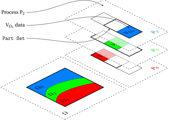
In order to distribute linear system which originates from the discretization of a PDE on a domainΩ (see §1.1.1), we identify D_ΩIwith a uniqueIDand we call this structure (along with some additional information about overlaps; see §2.3) aPart. Each part is associated with a unique processor, therefore we can summarise that in ADDMlib the discretized domain D_Ω, decomposed into N subdomains , has its representation in N uniquePartsand their associated data can be stored on p (1 ≤ p ≤ N) processes.

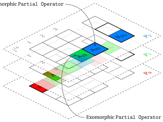
A local data structure must be set up in each processor to allow basic operation, such as (global) matrix-vector product and preconditioning operations, to be performed efficiently. Hence global operator is divided into sparse Partial Operators which act on Partial

Vectorsi.e., components of global vector. For future explanation see §2.2.

It is important to preprocess the distributed data in order to facilitate the implementa-tion of the communicaimplementa-tion tasks and to gain efficiency during the iterative process. The im-portant observation is that a given process does not need to store information about global

structure of decomposed system. It is optimal to reduce information to neighboringParts4

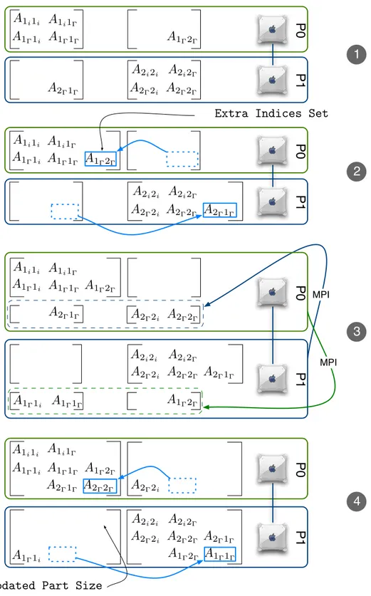
since data exchange processes only through common interface between subdomains. Thus the preprocessing requires setting up for each process a “Part Set” object, which is a list of localPartsandPart Infosof their neighbors. WherePart Infois a container of essential and cheap to store, information about non localPart.

Since thePartis a fundamental constituent of domain decomposition realization in AD-DMlib, the communication classes5implemented in ADDMlib support us in developing al-gorithms focused on data exchange between them, keeping informations about their physi-cal distribution oven a cluster of processes hidden. In other words we can first decide what data should be exchange between givenParts(domain decomposition algorithm level) and then by using theirIDsand ADDMlib interface for MPI we can easily establish data transfer between associated processes using point-to-point communication (data exchange between distributed memory).

2.2 Linear Algebra

The core object models for modern linear solver library consists of base classes captur-ing the mathematics, i.e.,Matrix,Vector,Iterative SolverandPreconditioner. Their structures should be motivated by parallel architecture on which we plan to solve our prob-lem and by operations we want to perform in order to obtain solution.

When we consider Krylov subspace techniques, namely, the preconditioned generalized minimal residual (GMRES) algorithm for the nonsymmetric case (or its flexible variant FGM-RES), it is easy to notice that all Krylov subspace techniques require the same basic opera-tions, thus the first step when implementing those algorithms on a high performance com-puter is identifying main operations that they require. We can list them after [51]:

◦ vector updates ◦ dot products

◦ matrix by vector multiplication ◦ preconditioner setup and operations.

For the sake of straightforward presentation, this section is divided into four logical parts; Vector, Matrix, Iterative Solver and Preconditioner. In each section emphasis is placed on concise description of data structures and algorithms used in implementation of associated elements and their basic algebra in ADDMlib.

4. In this case, neighboring in algebraic sense i.e., the twoPartsare neighbour when they have a common interface. Thus process on which neighbours data structures are stored, can be physically very remote.

5. ADDMlib has object oriented interface for MPI (which is procedural in nature) in order to simplify and encapsulate typical communication tasks (e.g., sending a block of data to pointed process)