HAL Id: tel-00008759
https://tel.archives-ouvertes.fr/tel-00008759
Submitted on 11 Mar 2005HAL is a multi-disciplinary open access
archive for the deposit and dissemination of sci-entific research documents, whether they are pub-lished or not. The documents may come from teaching and research institutions in France or abroad, or from public or private research centers.
L’archive ouverte pluridisciplinaire HAL, est destinée au dépôt et à la diffusion de documents scientifiques de niveau recherche, publiés ou non, émanant des établissements d’enseignement et de recherche français ou étrangers, des laboratoires publics ou privés.
Thomas Boulogne
To cite this version:
Thomas Boulogne. Nonatomic strategic games and network applications. Mathematics [math]. Uni-versité Pierre et Marie Curie - Paris VI, 2004. English. �tel-00008759�
TH`ESE DE DOCTORAT DE L’UNIVERSIT´E PARIS 6
Sp´ecialit´e : MATH´EMATIQUES APPLIQU´EES
pr´esent´ee par
Thomas BOULOGNE
pour obtenir le grade de Docteur de l’UNIVERSIT´E PARIS 6
Jeux strat´
egiques non-atomiques
et
applications aux r´
eseaux
Soutenue le 15 d´ecembre 2004 devant le jury compos´e de : MM. Eitan Altman Directeur
Guillaume Carlier Examinateur Jean Fonlupt Examinateur St´ephane Gaubert Examinateur Sylvain Sorin Directeur Nicolas Vieille Rapporteur Bernhard Von Stengel Rapporteur
Table des mati`
eres / Contents
Introduction 7
Bibliographie . . . 14
I
Nonatomic strategic games
15
Notations 17 1 Two models of nonatomic games 19 1.1 The assumption of nonatomicity . . . 191.2 S-games . . . 20
1.2.1 Payoff functions defined on S× FS . . . 20
1.2.2 Payoff functions defined on S× co(S) . . . 24
1.3 M-games . . . 26
1.4 Relations between S-games and M-games . . . 29
1.4.1 From S-games to M-games . . . 30
1.4.2 From M-games to S-games . . . 32
2 Approximation of large games by nonatomic games 37 2.1 S-games and λ-convergence . . . 38
2.2 S-games and convergence in distribution . . . 45
2.3 M-games and weak convergence . . . 47
3 Extensions and variations 53 3.1 Extensions of S-games . . . 53
3.2 Extension of M-games . . . 54
3.3 Population games . . . 57
3.4 Potential games . . . 60
3.4.1 Infinite potential games . . . 61
3.4.2 Potential games as limits of finite player games . . . 62
4 Applications 69 4.1 Routing games . . . 69
4.1.1 Nonatomic routing games . . . 69
4.1.2 Approximation of Wardrop equilibria by Nash equilibria . . . 72
4.2 Crowding games . . . 74
4.2.1 Large crowding games . . . 75
4.2.2 Approximation . . . 76
4.3 Evolutionary games . . . 77
4.3.1 From Nash to Maynard Smith: different interpretations of Nash equilibrium . . . 78
4.3.2 Games with a single population . . . 79
4.3.3 Stability in games with n-populations . . . 84
5 Equilibrium’s refinement: stability 87 5.1 S-games . . . 87
5.2 Potential games . . . 91
5.3 Stability based on a recursive process . . . 94
Appendix 97 A Referenced theorems . . . 97 B Measurability conditions . . . 100 C Proof of Proposition 2.24 . . . 101 Bibliography . . . 103 Glossary of Symbols 107 List of definitions 109
II
Network applications
113
6 Mixed equilibrium for multiclass routing games 115 6.1 Introduction . . . 1156.2 Mixed equilibrium (M.E.): model and assumptions . . . 117
6.3 Existence of M.E. through variational inequalities . . . 119
6.4 Existence of M.E.: a fixed point approach . . . 121
6.5 Uniqueness of M.E.: Rosen’s type condition . . . 122
6.5.1 Sufficient condition for DSI . . . 126
6.6 Uniqueness of M.E.: linear costs . . . 127
6.7 Uniqueness of M.E.: positive flows . . . 128
6.8 Uniqueness of M.E. for specific topologies . . . 132
6.8.1 Parallel links . . . 133
6.8.2 Load balancing with unidirectional links . . . 135
6.8.3 Load balancing with a communication bus . . . 135
6.9 Conclusion . . . 136
Appendix . . . 137
A Constraints in general networks . . . 137
B Relation between a bidirectional link and a network of unidi-rectional ones . . . 138
C Proof of Lemma 6.8.2 . . . 138
7 On the convergence to Nash equilibrium in problems of distributed
computing 145
7.1 Introduction . . . 145
7.2 Model . . . 146
7.2.1 Nash equilibrium . . . 147
7.2.2 The Elementary Stepwise System . . . 148
7.3 A network with two processors . . . 148
7.4 Network with N users . . . 152
7.4.1 Uniqueness of Nash equilibrium . . . 152
7.4.2 A network with N processors: uniqueness . . . 153
7.4.3 Convergence of ESS . . . 153
Bibliography . . . 155
8 Competitive routing in multicast communications 159 8.1 Introduction . . . 159
8.2 Model . . . 161
8.3 Uniqueness of equilibrium: specific topologies . . . 166
8.3.1 A three nodes network . . . 166
8.3.2 A four nodes network . . . 171
8.4 Uniqueness of equilibrium: general topology . . . 174
8.4.1 Extended Wardrop equilibrium . . . 174
8.4.2 Nash equilibrium . . . 176
8.5 Numerical example . . . 177
8.6 Multicast networks with duplication at the source . . . 178
8.7 Conclusion, discussion and further extensions . . . 182
Introduction
La th´eorie des jeux est l’´etude de situations o`u plusieurs individus interagissent. Une interaction sp´ecifie le comportement de chaque individu et donne `a tous une utilit´e. Cette derni`ere se mesure par une fonction r´eelle, appel´ee fonction d’utilit´e ou fonction de paiement, que tout individu est suppos´e maximiser. Un individu est appel´e joueur et un comportement strat´egie. Formellement : I est l’ensemble des joueurs, Si l’ensemble de strat´egies du joueur i ∈ I et ui : S = Πi∈ISi → R est sa
fonction de paiement. Le triplet (I, (Si)i∈I, (ui)i∈I) constitue un jeu (strat´egique),
une interaction est d´ecrite par un profil de strat´egies s = (si)i∈I ∈ S.
Un concept fondamental dans les jeux strat´egiques est l’´equilibre de Nash ; il s’agit d’un profil de strat´egies tel qu’aucune d´eviation unilat´erale ne soit profitable au joueur d´eviant. Explicitement, s = (sj, s−j) est un ´equilibre de Nash du jeu
(I, (Si)i∈I, (ui)i∈I) si et seulement si
uj(s))≥ uj¡s′j, s−j¢ , ∀j ∈ I, s′j ∈ Sj.
Lorque le mot ´equilibre est employ´e ci-apr`es, il doit s’interpr´eter comme une varia-tion de l’´equilibre de Nash.
L’objet de cette th`ese est double. D’une part il consiste en l’analyse de jeux avec un continuum de joueurs o`u la strat´egie d’un de ceux-ci, quel qu’il soit, a une influence nulle sur la fonction de paiement de n’importe quel autre joueur. Ces jeux sont appel´es jeux non-atomiques.
L’usage des jeux non-atomiques permet d’obtenir des r´esultats comme l’existence d’´equilibre lorsque les ensembles de strat´egies sont finis (autrement dit ´equilibre en strat´egie pure, ce qui n’est g´en´eralement pas le cas pour les jeux avec un nombre fini de joueurs) et d’utiliser des outils d’analyse fonctionnelle.
Cependant, une infinit´e de joueurs (a fortiori un continuum) ne se rencontre pas “dans la r´ealit´e”. Les jeux non-atomiques sont donc utilis´es pour d´ecrire des interactions avec un grand nombre d’individus et o`u le comportement de quiconque a une influence n´egligeable sur le paiement des autres. Nous appelons ces jeux grands jeux.
Nous montrons que les jeux non-atomiques sont de bons mod`eles pour analyser les grands jeux. Ceci est ´etabli en consid´erant des suites de jeux avec un nombre fini de joueurs, o`u l’influence d’un joueur s’evanouit lorsque le nombre de joueurs augmente (dor´enavant hypoth`ese d’´evanescence). Puis, nous ´etudions diverses appli-cations des jeux non-atomiques. Enfin, nous proposons un raffinement de l’´equilibre que nous appelons stabilit´e. Ceci constitue la premi`ere partie de cet ouvrage.
L’autre volet de ce manuscrit consid`ere des probl`emes dans les domaines des t´el´ecommunications et de l’Internet, autrement dit des r´eseaux, dans une optique de th´eorie des jeux. Sont consid´er´es des mod`eles o`u un grand nombre de paquets (dans le cadre du trafic routier, ceux-ci correspondent `a des v´ehicules), mod´elis´e par un continuum, doivent aller d’un point du r´eseau `a un autre. Pour ce faire les paquets peuvent ˆetre d´elivr´es via diff´erents chemins (routes) possibles. Tout chemin pr´esente un coˆut d´ependant de sa fr´equentation ou plus g´en´eralement de la r´epartition des paquets au travers des diff´erents chemins. Les d´ecisions de routage, c’est-`a-dire le choix des routes pour les paquets, peuvent se faire de trois mani`eres diff´erentes : (1) la d´ecision centralis´ee : une entit´e organise la circulation des paquets afin de minimiser le coˆut total de transport,
(2) la d´ecision group´ee : les paquets sont group´es, chaque groupe ayant un d´ecideur qui essaie de minimiser le coˆut de “son” groupe,
(3) la d´ecision individuelle : chaque paquet poss`ede son propre d´ecideur qui choisit son chemin afin de minimiser son coˆut.
Le premier cas est un probl`eme d’optimisation qui n’entre pas dans le cadre de la th´eorie des jeux et n’est donc pas consid´er´e ici. Les deux derniers cas sont des jeux o`u les joueurs sont les d´ecideurs et les fonctions de paiement sont les oppos´ees des fonctions de coˆut. Le cas (2) correspond `a un jeu avec un petit nombre de joueurs et le (3) `a un jeu non-atomique.
Nous proposons et ´etudions tout d’abord un concept d’´equilibre pour des mod`eles dans lesquels d´ecision group´ee et d´ecision individuelle coexistent : certains paquets se routent seul, d’autres s’en remettent `a une entit´e sup´erieure. Puis nous ´etablissons la convergence de syst`emes dynamiques vers des ´equilibres dans des jeux `a deux joueurs pr´esentant une architecture de r´eseaux sp´ecifique. Finalement, nous mod´elisons une situation propre aux r´eseaux de communications o`u les paquets doivent aller d’une origine `a plusieurs destinations.
PARTIE 1 : JEUX STRAT´EGIQUES NON-ATOMIQUES
Le premier objectif de cette partie est de montrer que les mod`eles de jeux non-atomiques propos´es par Schmeidler (1973) et Mas-Colell (1984) constituent de bons outils pour analyser des situations de jeux avec un grand nombre de joueurs satis-faisant l’hypoth`ese d’evanescence (grands jeux).
Un autre but est de pr´esenter un cadre englobant diverses applications des jeux non-atomiques, tels les jeux de routage, les jeux de foule et les jeux ´evolutionnaires et d’y ´etendre un concept propre `a ces derniers : la strat´egie evolutionnairement stable.
Chapitre 1 : Deux mod`eles de jeux non-atomiques
Apr`es avoir d´efini la non-atomicit´e, nous d´ecrivons les jeux non-atomiques in-troduits par Schmeidler (1973) (S-jeux) et ceux introduits par Mas-Colell (1984) (M-jeux). Pour ces deux types de jeux, tous les joueurs ont le mˆeme ensemble de strat´egies S, espace m´etrique compact.
Un S-jeu est caract´eris´e par une fonction u qui associe `a chaque joueur t0 ∈
INTRODUCTION 9
fonction ut0 d´epend de la strat´egie de t0 et d’une fonction mesurable f associant `a
chaque joueur t∈ T une strat´egie st ∈ S. Une fonction f d´ecrit une interaction et
se nomme profil de strat´egies.
Dans un M-jeu, les fonctions de paiement d´ependent de la strat´egie du joueur concern´e et de la r´epartition des strat´egies au sein de la population. Plus pr´ecis´ement, unM-jeu est d´ecrit par une probabilit´e sur l’ensemble des fonctions r´eelles continues sur S× M(S), not´e C(S × M(S)) (o`u M(X) est l’ensemble des probabilit´es sur X, muni de la topologie faible) et les interactions sont mod´elis´ees par des probabilit´es sur l’ensemble produit C(S× M(S)) × S.
Losque les S-jeux et les M-jeux sont d´efinis sous les mˆemes hypoth`eses, nous ´etablissons les liens les unissant. Une des hypoth`eses pour les S-jeux est que la fonction de paiement de tout joueur d´epend d’un profil de strat´egies f uniquement `a travers sa distribution -ou mesure image- f [λ] = λ◦ f−1 ∈ M(S) (le jeu est alors
dit anonyme). Nous montrons que
(i) la measure image u[λ] d’un S-jeu anonyme u est un M-jeu,
(ii) la measure image (u, f )[λ] de u et d’un de ses ´equilibres f est un ´equilibre pour leM-jeu u[λ].
R´eciproquement nous ´etablissons la repr´esentation desM-jeux (et de leurs ´equili-bres) par desS-jeux anonymes. Ce dernier r´esultat est une application du th´eor`eme de repr´esentation de Skorohod.
Chapitre 2 : Approximation des grands jeux par les jeux non-atomiques Nous appelons suite ´evanescente de jeux, une suite de jeux avec un nombre fini de joueurs (dor´enavant jeux finis), telle que l’influence de tout joueur sur le paiement des autres s’´evanouit lorsque le nombre de joueurs augmente. Nous consid´erons tou-jours des jeux finis o`u tous les joueurs ont le mˆeme ensemble de strat´egies S.
Il est montr´e ici que les jeux non-atomiques constituent un cadre ad´equat pour analyser les grands jeux.
Pour ce faire, nous pr´esentons trois r´esultats d’approximation correspondant aux trois formulations de jeux finis suivantes.
Forme adapt´ee 1 : o`u l’ensemble des joueurs est plong´e dans l’intervalle [0, 1] = T .
Les profils de strat´egies y sont des fonctions f adapt´ees `a une certaine partition Tn
de T . Le jeu est alors repr´esent´e par une fonction u adapt´ee `aTn.
Forme quasi-normale : Pn = {1, . . . , n} est l’ensemble des joueurs, un profil de
strat´egies est une fonction de Pn dans S. Le jeu est d´ecrit par une fonction qui
associe `a chaque joueur i sa fonction de paiement ui : Sn → R.
Forme probabiliste : les fonctions de paiement sont d´efinies sur S× M(S), et le jeu est donn´e par une probabilit´e atomique µ sur l’ensemble de ces fonctions.
A la forme adapt´ee, nous associons une convergence “uniforme”, `a la forme quasi-normale, la convergence en distribution utilis´ee par Hildenbrand (1974) et `a la forme probabiliste, la convergence faible des mesures. Les deux premi`eres approximations concernent les S-jeux, la derni`ere les M-jeux. Les r´esultats obtenus sont du type suivant.
1
Etant donn´ee une partition mesurableT de T , une fonction ϕ ayant pour domaine de d´efinition T et constante sur chaque ´el´ement deT est appel´ee fonction adapt´ee `a la partition T .
Soient une suite ´evanescente de jeux Gn qui converge vers un jeu non-atomique
G et une suite d’interactions ϕn de Gn qui converge vers une interaction ϕ de G.
Alors
(1) si ϕnest un ´equilibre de Gn, pour un nombre infini de n, alors ϕnest un ´equilibre de G et inversement,
(2) si ϕ est un ´equilibre de G alors pour n assez grand ϕn est “approximativement”
un ´equilibre de Gn.
Chapitre 3 : Extensions et variations
Ce chapitre pr´esente tout d’abord des r´esultats sur l’extension desS-jeux anony-mes ´etablis par Rath (1992) et Khan-Sun (2002), puis ´etend les M-jeux `a des situ-ations o`u
(i) l’ensemble des joueurs est partionn´e en un nombre fini de populations, chaque population ayant son propre ensemble de strat´egies,
(ii) les fonctions de paiement d´ependent des r´epartitions des strat´egies au sein de chaque population.
Les jeux ainsi d´efinis sont appel´es C-jeux. Nous montrons l’existence d’´equilibre pour les C-jeux de deux mani`eres diff´erentes. La premi`ere consiste en l’application classique d’un th´eor`eme de point-fixe `a une correspondance de meilleures r´eponses (ses points fixes sont des ´equilibres). La seconde consid`ere une fonction allant de l’ensemble desC-jeux dans celui des M-jeux et montre qu’`a un ´equilibre d’un M-jeu µ correspond un ´equilibre du C-jeu dont µ est l’image par la fonction mentionn´ee ci-dessus.
Nous nous restreignons ensuite `a une classe de C-jeux o`u tous les joueurs d’une mˆeme population ont la mˆeme fonction de paiement. Dans ces jeux, appel´es jeux de population, l’existence d’´equilibre peut s’obtenir `a l’aide d’in´egalit´es variationnelles. Comme il est montr´e dans le chapitre 4, ces jeux englobent diverses applications des jeux non-atomiques.
Finalement, nous pr´esentons une sous-classe des jeux de population, les jeux de potentiel introduits par Sandholm (2001). Ces jeux ont la propri´et´e de poss´eder une fonction, appel´ee fonction de potentiel, dont les maxima sont des ´equilibres du jeu consid´er´e. Sandholm (2001) ´etablit un r´esultat d’approximation des jeux de poten-tiel avec un nombre fini de joueurs par les jeux de potenpoten-tiel avec un continuum de joueurs. Nous montrons que ce r´esultat est plus restrictif que les approximations obtenues au chapitre 2.
Chapitre 4 : Applications des jeux non-atomiques
Ce chapitre est consacr´e `a l’´etude de trois types de jeux de population.
Les jeux de routage sont tout d’abord consid´er´es. Le contexte est celui d’un trafic routier et un jeu mod´elise des situations o`u un grand nombre de v´ehicules doivent aller d’une origine `a une destination. Pour ce faire ils ont plusieurs routes possibles et chacun d´esire minimiser son temps de trajet, temps qui d´epend de la route choisie et de sa fr´equentation. Nous sommes donc dans le cas de d´ecision individuelle d´efinie au d´ebut de l’introduction. La solution d’´equilibre dans ces jeux remontent `a Wardrop (1952). Nous pr´esentons un r´esultat d’approximation des ´equilibres des jeux de routage finis (d´ecision group´ee) par l’´equilibre de Wardrop dˆu
INTRODUCTION 11
`a Haurie et Marcotte (1985).
Ensuite, sont ´etudi´es les jeux de foule, introduits par Milchtaich (2000). Il s’agit d’une extension des jeux de congestion `a n joueurs d´efinis par Rosenthal (1973). Etant donn´e le choix d’une strat´egie, la fonction de paiement d’un joueur d´epend du “nombre” de joueurs ayant adopt´e cette strat´egie et est continuement d´ecroissante. Il s’agit donc d’un cas particulier de jeu de routage. Nous pr´esentons un r´esultat de Milchtaich (2000) sur l’approximation de jeux finis par les jeux de foules.
Finalement, sont analys´es les jeux ´evolutionnaires. Ils sont issus de la biolo-gie ´evolutionnaire et remontent `a Maynard Smith-Price (1973) et Maynard Smith (1974). Ils mod´elisent l’´evolution des caract`eres au sein d’une esp`ece et abandonnent l’hypoth`ese de rationalit´e des joueurs, traditionnelle en th´eorie des jeux. Ces mod`eles consid`erent des interactions entre individus d’une mˆeme esp`ece (ou population) qui se font de mani`ere r´ep´et´ee ; chaque individu a une strat´egie fix´ee (un caract`ere) et son taux de reproduction d´epend du paiement qu’il obtient au cours des interac-tions. Une probabilit´e sur l’ensemble des strat´egies repr´esente donc une r´epartition des caract`eres au sein de l’esp`ece ou encore une composition de la population. Ainsi plus une caract´eristique est efficace pour une composition de la population, plus elle aura tendance `a ˆetre repr´esent´ee. Un ´equilibre dans ces jeux correspond `a une situation o`u chaque caract´eristique a le mˆeme taux de reproduction : il d´etermine donc une composition “stable” de la population. Mais cette stabilit´e peut s’av´erer tr`es sensible aux petites perturbations de la population (comme les mutations). C’est pourquoi la th´eorie des jeux ´evolutionnaires s’int´eresse au concept de strat´egie ´evolutionnairement stable qui d´efinit des compositions de population robustes aux changements lorsqu’ils sont suffisamment petits.
Chapitre 5 : Raffinement de l’´equilibre : la stabilit´e
Ce chapitre conclut la premi`ere partie en ´etendant la notion de strat´egie ´evolu-tionnairement stable auxS-jeux d´efinissant ainsi les profils de strat´egies stables. Un profil de strat´egies est stable si, pour toute d´eviation d’un ensemble de joueurs de mesure “faible”, ´etant donn´e le nouveau profil, la moyenne des paiements de ces joueurs est plus faible que la moyenne des paiements obtenus s’ils n’avaient pas d´evi´e individuellement. Formellent, f est stable pour le S-jeu u s’il existe ¯ε > 0 tel que, pour tout sous-ensemble Tε de T de measure ε < ¯ε et pour tout profil g avec
g(t) = f (t) pour tout t∈ T \ Tε, Z Tε ut(f (t), g) dλ(t) > Z Tε ut(g(t), g) dλ(t).
Nous montrons d’abord qu’un profil de strat´egies stable dans un S-jeu u est un ´equilibre. Puis, ´etant donn´es un S-jeu et une suite de jeux sous forme adapt´ee un
convergeant vers u, nous caract´erisons l’ensemble des profils de strat´egies stables de u comme les points limites de suites d’´equilibres stricts fnde un. Ensuite, nous nous
pla¸cons dans le cadre des jeux de potentiel afin d’´etudier les relations entre stabilit´e et maxima des fonctions de potentiels. Finalement, nous pr´esentons un processus de s´election de profils de strat´egies dont les solutions sont stables.
PARTIE 2 : APPLICATIONS DE LA TH´EORIE DES JEUX AUX R´ESEAUX
Cette partie est constitu´ee de trois articles ayant trait aux probl`emes de mod´elisation du routage dans des r´eseaux.
Un r´eseau est un graphe orient´e fini dans lequel un continuum de paquets doivent circuler. A chaque paquet est associ´e un couple de sommets (origine-destination). Les paquets ont diff´erents chemins `a leur disposition et tout chemin a un coˆut d´ependant de la r´epartition des paquets dans le graphe. Ce coˆut peut repr´esenter par exemple un temps de transport ou une probabilit´e de perte. Le graphe constitue l’architecture du r´eseau.
Nous consid´erons deux types de d´ecision d´efinis au d´ebut de l’introduction : d´ecision group´ee et d´ecision individuelle. Le premier type d´efinit un jeu avec un nombre fini de joueurs o`u le concept de solution ´etudi´e est l’´equilibre de Nash. Pour le deuxi`eme (un jeu non-atomique), le concept de solution adopt´e est l’´equilibre de Wardrop : tout chemin utilis´e doit avoir un coˆut moindre que n’importe quel autre chemin (ayant mˆeme origine-destination).
Chapitre 6 : L’´equilibre mixte dans les jeux de routage
Pla¸cons nous dans un contexte de trafic routier afin d’expliquer le probl`eme mod´elis´e dans ce chapitre.
Soit un r´eseau o`u de nombreux v´ehicules doivent aller d’une origine `a une destina-tion, tous voulant minimiser leur temps de trajet. Origines et destinations d´ependent des v´ehicules mais sont en nombre fini. Un v´ehicule peut soit d´eterminer seul son itin´eraire (d´ecision individuelle), soit s’abonner `a un syst`eme de guidage qui lui recommande un itin´eraire (d´ecision group´ee). On suppose que les abonn´es suivent la proposition conseill´ee et que tout syst`eme de guidage cherche `a minimiser le temps de trajet moyen de ses clients.
Nous mod´elisons cette situation par un jeu compos´e de deux types de joueurs : des “gros” joueurs repr´esentant les syst`emes de guidage et des “petits” joueurs cor-respondant aux v´ehicules “‘ind´ependants”. L’ensemble des gros joueurs,N , est fini, celui des petits joueurs,W, est un continuum. Une strat´egie d’un gros joueur i ∈ N est le choix d’une r´epartition de ses paquets au travers des differentes routes : Si
est donc le simplexe de Rki (k
i ´etant le nombre de chemins possibles pour i). Celle
d’un petit joueur est le choix d’un itin´eraire. Supposons pour all´eger la pr´esentation que tous les petits joueurs ont les mˆemes origine, destination, ensemble de chemins Sw et fonction de coˆut uw. Sw consiste en la base canonique de Rkw. Ce jeu peut
s’´ecrire sous la forme (N , W, (Si)i∈N, Sw, (ui)i∈N, uw) o`u ui est la fonction de coˆut
du joueur i ∈ N .
Nous d´efinissons un concept d’´equilibre pour de tels jeux : l’´equilibre mixte. Nous montrons son existence pour des architectures quelconques de deux mani`eres diff´erentes. La premi`ere consiste en la caract´erisation de l’´equilibre en termes d’in´ega-lit´es variationnelles, du type
F (x)· (y − x) ≥ 0, ∀y ∈ X = Πi∈NSi× co(Sw)⊂ Rn,
o`u F : X ⊂ Rn → Rn et co(S
w) est l’enveloppe convexe de Sw. L’existence d’une
INTRODUCTION 13
et born´e. La deuxi`eme d´ecompose, dans un premier temps, le jeu en deux sous-jeux, l’un, (N , (Si)i∈N, (ui)i∈N), compos´e des gros joueurs et l’autre, (W, Sw, uw),
des petits joueurs. Il est ensuite montr´e que le jeu non-atomique (W, Sw, uw) admet
une fonction de potentiel ϕ. Finalement, l’on construit un jeu `a #N +1 joueurs pour lequel le #N + 1`emejoueur a pour ensemble de strat´egies co(S
w) et pour fonction de
coˆut ϕ. Un ´equilibre de Nash de ce jeu est alors un ´equilibre mixte du jeu originel. Ensuite, nous ´etablissons des conditions pour l’unicit´e de l’´equilibre mixte. L’uni-cit´e de l’´equilibre de Nash ´etant rare, nous ne pouvons nous attendre `a obtenir celle de l’´equilibre mixte sans certaines restrictions. Nous l’obtenons pour
(i) des fonctions de coˆut sp´ecifiques et des architectures quelconques, (ii) des architectures simples et des fonctions de coˆut g´en´erales.
Chapitre 7 : Convergence vers l’´equilibre de Nash dans un probl`eme de syst`emes distribu´es
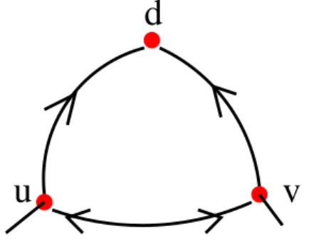
Nous consid´erons des jeux de routage avec deux types d’architectures dans lesquel-les tous lesquel-les arcs possiblesquel-les pointant vers un sommet sp´ecifique d sont pr´esents.
Dans la premi`ere architecture, les autres sommmets sont au nombre de deux et sont reli´es par une arˆete (arc non orient´e). Dans la deuxi`eme, les autres sommets (n) forment un circuit orient´e.
Dans les deux r´eseaux le sommet d est la destination commune `a tous les joueurs. A chaque sommet diff´erent de d est associ´e un joueur. Tout joueur a un continuum de paquets `a router vers d. Nous sommes donc dans le cas de d´ecisions group´ees.
Pour chacun des jeux, nous montrons l’unicit´e de l’´equilibre de Nash. Par la suite, nous ´etudions la convergence d’un algorithme de meilleure r´eponse o`u les joueurs actualisent leur strat´egie `a tour de rˆole. La convergence est due, dans le premier jeu, `a la monotonie de la suite engendr´ee par l’algorithme et, dans le deuxi`eme, `a la contraction des ´ecarts entre deux pas cons´ecutifs de l’algorithme. De plus, pour le premier jeu, nous ´etendons la convergence `a deux autres types d’algorithme.
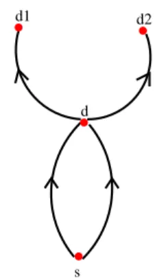
Chapitre 8 : Routage dans des r´eseaux de t´el´ecommunications multipoint Ce dernier chapitre traite de la mod´elisation par la th´eorie des jeux d’une situa-tion de communicasitua-tion multipoint : les paquets doivent aller d’une origine `a plusieurs destinations. Pour ceci, les paquets peuvent se d´edoubler `a chaque noeud du r´eseau. Nous mod´elisons cette situation par un jeu `a n joueurs o`u la d´ecision d’un joueur consiste en la r´epartition de ses paquets au travers de chemins multipoints virtuels repr´esent´es par des arbres. Dans un arbre, tout joueur envoie uniquement une copie de chaque paquet, le r´eseau dupliquant l’information aux sommets appropri´es. Cette construction rend caduc les m´ethodes utilis´ees pour les communications de point-`a-point.
Nous analysons trois types de fonctions de coˆut, puis nous d´efinissons l’´equilibre de Nash de ce jeu et ´etudions son unicit´e. Celle-ci est obtenue pour des fonctions de coˆut g´en´erales et des architectures sp´ecifiques (et inversement). Nous ´etablissons ´egalement la convergence vers l’´equilibre d’une dynamique de meilleures r´eponses sous des conditions sur les coˆuts et les architectures. Une des fonctions de coˆut ´etudi´ees permet d’itentifier ´equilibre de Nash et ´equilibre de Wardrop. Ainsi dans ce cadre, l’unicit´e de l’´equilibre de Nash et la convergence vers celui-ci de dynamiques
du type Brown-Von Neumann (1950) sont obtenus.
Bibliographie
[1] G. Brown and J. Von Neumann. Solutions of games by differential equations. In H. Kuhn and A. Tucker, editors, Contributions to the Theory of Games I, Annals of Mathematics Studies 24, pages 73–79. Princeton University Press, 1950.
[2] A. Haurie and P. Marcotte. On the relationship between Nash-Cournot and Wardrop equilibria. Networks, 15:295–308, 1985.
[3] W. Hildenbrand. Core and Equilibria of a Large Economy. Princeton University Press, 1974.
[4] M. Khan and Y. Sun. Non-cooperative games with many players. In R. Aumann and S. Hart, editors, Handbook of Game Theory, volume 3, pages 1761–1808. Elsevier Science, 2002.
[5] A. Mas-Colell. On a theorem of Schmeidler. Journal of Mathematical Economics, 13:201–206, 1984.
[6] J. Maynard Smith. The theory of games and the evolution of animal conflicts. Journal of Theoretical Biology, 47:209–221, 1974.
[7] J. Maynard Smith and G. Price. The logic of animal conflict. Nature, 246:15–18, 1973.
[8] I. Milchtaich. Generic uniqueness of equilibrium in large crowding games. Mathemat-ics of Operations Research, 25:349–364, 2000.
[9] K.P. Rath. A direct proof of the existence of pure strategy equilibria in games with a continuum of players. Economic Theory, 2:427–433, 1992.
[10] R.W. Rosenthal. A class of games possesing pure-strategy Nash equilibria. Interna-tional Journal of Game Theory, 2:65–67, 1973.
[11] W.H. Sandholm. Potential games with continuous player sets. Journal of Economic Theory, 97:81–108, 2001.
[12] D. Schmeidler. Equilibrium points of nonatomic games. Journal of Statistical Physics, 7:295–300, 1973.
[13] J.G. Wardrop. Some theoretical aspects of road traffic research. Proc. Inst. Civ. Eng., Part 2, 1:325–378, 1952.
Part I
Nonatomic strategic games
Notations
For any metric space S, B(S) denotes the Borel σ-algebra on S, and M(S) the set of probabilities on B(S). By a probability µ on S we shall understand an element of M(S).
Let A be a finite set: A ={1, . . . , m}. It is identified with the standard basis of Rm
consisting of the coordinate axes: Each element a∈ A is send to the vector δa ∈ Rm,
defined by δa=
n1 if a = b, 0 otherwise.
In other terms, δa is the Dirac measure on a. Thus the convex hull of A, denoted
by co(A)(=M(A)) is identified with the simplex ∆m = ∆ of Rm.
For any compact set X, the space a real-valued continuous functions on X is denoted by C(X).
For a set B, 1B denotes the indicator function of B.
The inner product in Rm is denoted by· and its euclidean norm by k · k.
The notation := indicates a definition.
A superscript refers to the set of actions, whereas a subscript refers to the set of players.
When a reference is made to a lemma, a proposition, a theorem, . . ., the first character refers to the chapter, for example Theorem 1.5 is located in Chapter 1, if the character is not a number but a letter, then the location is in the corresponding appendix for example Theorem A.15 is located in Appendix A.
Chapter 1
Two models of nonatomic games
In this chapter, first is defined nonatomic measure space a key notion of nonatomic games. Then two models of nonatomic games in which all players have same strategy set are described. They differ on the notion of strategy and on the set on which payoff functions are defined.
The first one is due to Schmeidler (1973): a strategy profile is a class of equiv-alence of measurable functions from the player set to the strategy set. The payoff function of a player, defined in a great generality, depends on his strategy and on the strategy profile played. We call these games S-games.
The second one is due to Mas-Colell (1984)1 : the main concern is not strategy
profiles but probabilities over the product space (payoff function-strategy). There-fore payoff functions do not depend on the strategy profile played but only on the measure induced by this last. We call these gamesM-games.
Section 1.2 presents S-games and gives the proofs of equilibrium’s existence in mixed and also in pure strategies. Section 1.3 deals with M-games, proofs of equi-librium’s existence are also given.
Finally Section 1.4 establishes relations betweenS-games and M-games. Namely, when both games satisfy common assumptions, it is shown that anyS-game induces an M-game and that any M-game can be represented by an S-game and a corre-spondence between equilibria ofS-games and equilibria of M-games is established.
1.1
The assumption of nonatomicity
We consider games with many players, where the strategy of any single player has a negligible influence on the payoff of the other players, but strategies of a group of players can affect any payoff functions. Thus, given a profile of players’ strategies, if a player changes his strategy, he is the only one whose payoff may be concerned by this change. To describe such games we assume that the set of players is a nonatomic (or atomless) measure space:
1.1. Definition. Let (T,T , λ) be a measure space where T is a set, T is a σ-algebra 1
All the references to Schmeidler and Mas-Colell will be to, respectively, Schmeidler (1973) and Mas-Colel (1984).
of subsets of T , and λ is a measure on T ; (T, T , λ) is nonatomic if
∀E ∈ T such that λ(E) > 0, ∃F ⊂ E ∈ T such that 0 < λ(F ) < λ(E).
If (T,T , λ) is nonatomic, then T is uncountable. On the other hand, if T is an uncountable complete separable metric space, then there exists a nonatomic measure on the Borel σ-algebra of T (Parthasarathy, 1967, Theorem 8.1, p. 53).
We restrict our attention to the measure space of players (T,B(T ), λ) where T := [0, 1] and λ is Lebesgue measure; it is denoted T := (T,B(T ), λ).
1.2
S-games
Let S be a set of strategies, S is a compact subset of Rm.
1.2. Definition. A strategy profile is an equivalent class f of measurable functions from T to S. FS denotes the set of strategy profiles.
1.3. Definition. An S-game is defined by a triple (T , FS, (ut)t∈T), where T =
(T,B(T ), λ) is the measure space of players, and ut : S × FS → R is the payoff
function of player t, for each t∈ T .
Schmeidler extended the notion of Nash equilibrium toS-games as follows: 1.4. Definition. A strategy profile f of theS-game (T , FS, (ut)t∈T) is an equilibrium
strategy profile if
∀y ∈ S, ut(f (t), f )≥ ut(y, f ), for λ-a.e. t∈ T.
To prove the existence of an equilibrium strategy profile in an S-game
(T ,FS, (ut)t∈T), we will define as usual a correspondence α whose fixed points will
be equilibria. To apply fixed point theorems requires some assumptions on (i) the strategy set S, (ii) the set of strategy profiles FS and (iii) the payoff functions ut.
We will present two sets of assumptions under which an S-game has an equilibrium strategy profile.
1.2.1
Payoff functions defined on S
× F
SLet A = {1, . . . m} be a finite action set, it is identified with the standard basis of Rm (see page 17). Let S be the set of mixed strategies, then it is the simplex
∆m = ∆ of Rm, hence a convex, compact subset of Rm. Moreover for all t∈ T , the
payoff function ut can be defined for all x∈ ∆ and f ∈ F∆ as
ut(x, f ) :=
X
a∈A
1.2. S-GAMES 21 In other words, for all t∈ T and f ∈ F∆, ut(·, f) is linear.
For a ∈ A, fa is Lebesgue integrable. Then F
∆ is a subset of L1(λ, Rm) that
we endow with the weak topology. For any subset Z ∈ T , write R
Zf for the vector
¡R
Zf
a(t) dλ(t)¢
a∈A.
Under the following conditions of continuity and measurability: (a) for all t∈ T and a ∈ A, ut(a,·) is continuous on F∆,
(b) for all f ∈ F∆and a, b∈ A, the set {t ∈ T ; ut(a, f ) > ut(b, f )} is measurable,
Schmeidler shows the existence of an equilibrium strategy profile using Fan-Glicksberg fixed point theorem (Theorem A.1).
1.5 Theorem. (Schmeidler, 1973, Theorem 1)
An S-game (T , F∆, (ut)t∈T) fulfilling conditions (a) and (b) has an equilibrium
strat-egy profile.
The proof given follows the lines of (Khan, 1985, Theorem 4.1.)’s proof. It explicits two points of the original one. Namely,
(i) We show that F∆ is weakly compact, this is the next proposition.
(ii) We explain why a sequence of F∆ instead of a net can be used to prove the
upper semicontinuity of a correspondence from F∆ to itself.
The specificity of these two points, compared to the proof of existence of Nash equilibrium for finite-player games, lays in the fact thatF∆is a subset of an infinite
dimensional vector space.
1.6 Proposition. F∆ is weakly compact.
Proof: From Dunford-Pettis’ theorem (Theorem A.2), to show that F∆ is weakly
compact, it is enough to show that F∆ is weakly closed. Due to the convexity
of F∆, this is equivalent to show, as stated by Mazur’s theorem (Theorem A.3),
that F∆ is closed in the norm topology. Let {fn} be a norm convergent sequence
of F∆, and f be its limit, f belongs to L1(λ, Rm). From (Dunford and Schwartz,
1988, Theorem III.3.6), {fn} converges in measure to f. Now apply (Dunford and
Schwartz, 1988, Corollary III.6.3) to extract a subsequence {fn′} of the sequence {fn} which converges λ-almost everywhere to f. Finally note that ∆ is closed to
conclude that f (t) belongs to ∆, λ-almost everywhere, so f belongs to F∆.
Proof of Theorem 1.5: To establish the existence of an equilibrium we shall construct as usual a best reply correspondence and look for a fixed point of this correspondence. For all t ∈ T and f ∈ F∆, let BRt(f ) be the set of best reply strategies of t
against f , that is BRt(f ) :={x ∈ ∆; ut(x, f )≥ ut(y, f ), ∀y ∈ ∆}.
Consider the correspondence α :F∆ → F∆ with
α(f ) :={g ∈ F∆; g(t)∈ BRt(f ), for λ-a.e. t∈ T }.
A fixed point of α is an equilibrium strategy profile.
To apply Fan-Glicksberg fixed point theorem one needs to show that
1) F∆ is compact, nonempty and convex in a locally convex topological vector
2) For every strategy profile f ∈ F∆, the set α(f ) is convex and nonempty.
3) The correspondence α is upper semicontinuous.
1) The nonemptyness and convexity of F∆ are straightforward, its (weak)
com-pactness is established by Proposition 1.6. Moreover, from the definition of the weak topology, it follows that L1(λ, Rm) is a locally convex topological vector space
(Dunford and Schwartz, 1988, p. 419).
2) To prove the nonemptyness of α(f ) we shall construct a strategy profile be-longing to it. Consider a strategy profile f ∈ F∆. For any action a∈ A, define the
set
Ta:={t ∈ T ; ut(a, f )≥ ut(b, f ), ∀b ∈ A}.
This definition yields T = ∪a∈ATa and for all players t in Ta, the vector a belongs
to BRt(f ). Because of condition (b), Ta is measurable. Let
Z1 := T1 and Za:= Ta\ (∪a−1 b=1Tb).
The strategy profile g, defined by g(t) := a for t∈ Za, belongs to α(f ).
The convexity of α(f ) is due to the convexity of BRt(f ) for all t∈ T .
3) Claim 3 is the hard task, first we shall show that BRtis upper semicontinuous,
then we shall proceed by contradiction to establish the upper semicontinuity of α. The set ∆ being compact, the upper semicontinuity of BRtwill follow if BRt has
a closed graph in F∆× ∆ (Proposition A.4). For all a ∈ A, the function ut(a,·) is
continuous (condition (a)), therefore the payoff function ut: ∆× F∆ → R is jointly
continuous, hence BRt has a closed graph.
Similarly to show the upper semicontinuity of α is equivalent to show that it has a closed graph. Since the weak topology of an infinite dimensional normed vector space is not metrizable (Diestel, 1984, p. 10-11), one should have to consider a net to establish the closedness of the graph of α. Nevertheless the weak compactness of F∆ allows to consider a sequence instead of a net: Indeed, let {(fν, gν)} be a net
converging to (f0, g0), where gν ∈ α(fν) (we will have to show that g0 ∈ α(f0)). The
union of the net {(fν, gν)} and (f0, g0) is is relatively weakly sequentially compact
by virtue of Eberlein-Smulian’s theorem (Theorem A.5). Now use Theorem A.6 to extract a sequence {(fn, gn)} from {(fν, gν)} that weakly converges to (f0, g0).
From Proposition 1.6’s proof, it follows that g0(t) belongs to ∆, λ-almost
every-where.
We now show by contradiction that g0 ∈ α(f0). Assume that for a nonnull
measurable subset Z of T , the strategies of players in S are not best replies against the strategy profile f0, namely for all t ∈ Z, g0(t) /∈ BR
t(f0). For each t, the set
BRt(f0) is a convex hull of a subset of the set A. So there is a nonnull, measurable
subset V of Z and a subset {j1, . . . , jk} of A such that, for each t ∈ V ,
BRt(f0) = co({j1, . . . , jk}) and g0(t) /∈ BRt(f0).
Hence there exists y ∈ ∆ such that
1.2. S-GAMES 23 For example let ya = 1/(m− k) for all a 6= j
l, l = 1, . . . , k. Note that y does not
depend on t.
So the inner product y ·R
V g
0 is (strictly) positive, but for each g ∈ F
∆ with g(t)∈ BRt(f0) for t∈ V , y· Z V g = 0.
Now, {gn} weakly converges to g0, therefore R
V g 0 = limR V g n. Let Z V lim sup{gn(t)} := ½Z V
g; for λ-a.e. t in V, g(t) is a limit point of {gn(t)} ¾
.
Then (Aumann, 1965, Proposition 4.1) (Theorem A.9) 2, yields
lim Z V gn ⊂ Z V lim sup{gn(t)}.
But each limit point of{gn(t)} belongs to BR
t(f0) (BRtis upper semicontinous). Hence y·R V g 0 = y· limR V g n = 0, a contradiction.
The conditions of Fan-Glicksberg fixed point theorem are satisfied for α, thus there exists a strategy profile f ∈ F∆ such that f ∈ α(f), in other words f is an
equilibrium of (T ,F∆, (ut)t∈T).
Note that to prove the non-emptyness of α, we used the finiteness of the set of extremal points of ∆, and the linearity of ut(·, f). In other words, the fact that
players act in mixed strategies is essential to obtain an equilibrium strategy profile when ut is defined on ∆× F∆. Nevertheless Schmeidler establishes also the
exis-tence of a pure equilibrium strategy profile f if for every a ∈ A and λ-a.e. t ∈ T , ut(a,·) depends on f only through
R
T f . This will lead to consider the second set of
assumptions. Before to do this we reformulate the previous theorem.
Let E(S) denote the set of extremal points of S. An S-game (T , FS, (ut)t∈T)
where ut : S × FS → R has an equilibrium strategy profile if it satisfies the
condi-tions A.1-5 below.
A.1 S is a convex hull of a finite number of points {p1, . . . , pn} of Rm.
A.2 FS is endowed with the weak topology of L1(λ, Rm).
A.3 ut(x,·) is continuous for all t ∈ T and all x ∈ S.
A.4 ut(·, f) is linear for all t ∈ T and all f ∈ FS.
A.5 For all f ∈ F and pk, pl ∈ E(S), the set {t ∈ T ; ut(pk, f ) > ut(pl, f )} is
mea-surable.
2
1.2.2
Payoff functions defined on S
× co(S)
Consider the S-game (T , FS, (ut)t∈T), where ut is defined on S × co(S). In this
framework a strategy profile f ∈ FS is an equilibrium of (T ,FS, (ut)t∈T) if
∀y ∈ S, ut µ f (t), Z f ¶ ≥ ut µ y, Z f ¶ , for λ-a.e. t ∈ T. 1.7. Remark. On R f.
When S represents a finite set of actions A, then R fa is the weight of players
choosing action a, and R f = ¡R fa¢
a∈A gives the distribution of actions across the
player set.
When S represents a convex set of actions (for example a player is a firm and an element of S is a quantity of output), then R f is an average.
The next theorem due to Rath (1992) establishes that theS-game (T ,FS, (ut)t∈T) has an equilibrium strategy profile if
B.1 S is a compact subset of Rm.
B.2 ut is jointly continuous on S× co(S), where S and co(S) are endowed with the
euclidean metric.
B.3 The function t7→ ut is measurable, where the space of continuous functions on
S× co(S) is endowed with the supremum norm. 1.8 Theorem. (Rath, 1992, Theorem 2)
Let (T ,FS, (ut)t∈T) be an S-game satisfying assumptions B.1-3. Then
(T ,FS, (ut)t∈T) has an equilibrium strategy profile.
Proof: The proof is presented only for the case where S is the basis of coordinate axes of Rm, S = A. The convex hull of A is seen as the set of integrals of pure
strategy profiles, co(A) = ∆ ={R f; f ∈ FA}.
The set of best reply strategies of player t is now defined for a probability x∈ ∆ and is BRt(x) :={a ∈ A; ut(a, x)≥ ut(b, x), ∀b ∈ A}. The best reply correspondence
is α : ∆ → ∆, α(x) := Z T BRt(x) dλ(t) µ := ½Z f ; f (t)∈ BRt(x), λ-a.e. ¾¶ .
As in Theorem 1.5, one has to establish claims 1, 2 and 3, the only difference being that ∆ belongs to some finite euclidean space and this simplifies the proof.
1) ∆ is the unit simplex in Rm, thus a nonempty, convex and compact subset of
Rm.
2) The nonemptiness of BRt(x) comes from the finiteness of the strategy set A.
The same construction as in Theorem 1.5’s proof establishes that α is nonempty. The convexity of α follows from the nonatomicity of λ (Lyapounov’s theorem, see, e.g. (Aliprantis and Border, 1999, Theorem 12.33)).
3) The last claim is that α has a closed graph. In fact, since (i) 0≤ fa(t)≤ 1 for every t ∈ T , a ∈ A and f ∈ F
A and
1.2. S-GAMES 25 it follows from (Aumann 1976) (Theorem A.13) that α has a closed graph (integra-tion preserves upper semicontinuity).
It remains to apply Kakutani’s fixed point theorem 3 (see, e.g., (Berge, 1965, p.
183)) to α.
1.9. Remark. On the assumptions of measurability.
Rath (1995) shows that assumption B.3 implies assumption (b). The converse is not true as shown in Appendix B.
1.10. Example. S-games and equilibrium strategy profiles.
(A)Consider theS-game with three actions a, b and c, where each player has payoff functions u(a, f ) = µZ fa ¶2 + Z fb, u(b, f ) = Z fa+ µZ fb ¶2 and u(c, f ) = Z fc. The equilibrium strategy profiles of this S-game are
(i) the three constant pure strategy profiles: f ≡ a, g ≡ b and h ≡ c,
(ii) the constant mixed strategy profiles fε ≡ ((1 − ε)/2, (1 + ε)/2, 0), where −1 <
ε < 1 and
(iii) all the strategy profiles f such that R fa = (1− ε)/2, R fb = (1 + ε)/2 and
R fc = 0, for some −1 < ε < 1.
(B) Consider an action set A = {a, b} and define the payoff function of player t by ut(c, f ) =ktδc+R fk2 (k · k is here the euclidean norm of R2, and δc ∈ R2 the Dirac
measure on c), for c ∈ A f ∈ F∆ and t ∈ T . In the S-game (T , F∆, (ut)t∈T), any
player t6= 0 strictly prefers the action the most played. Thus the pure equilibrium strategy profiles are
(i) the constant functions f ≡ a and g ≡ b and
(ii) those where half of the players chooses action a and the other half action b. Are also equilibria
(iii) the constant mixed strategy profile where all players select the mixed strategy (1/2, 1/2) and
(iv) all the strategy profiles f that satisfyR fa=R fb (for example f (t) = (1/4, 3/4),
for t∈ [0, 1/2) and f(t) = (3/4, 1/4), for t ∈ [1/2, 1]).
S-games constitute an exhaustive framework to analyse interactions with a large number of individuals. Indeed, a pair (f, (ut)t∈T) gives t’s strategy and t’s payoff
function, moreover this payoff function may depend on the entire strategy profile. First this exhaustiveness may be unrealistic in many game’s situation (e.g., conges-tion games, market games, populaconges-tion games) where (i) players are affected by a strategy profile only through the measure it induces on the strategy set as in section 1.2.2 and (ii) only this measure is known and not each individual’s behavior. Second from a mathematical point of view, the set of strategy profiles FS is very big, and
thus is not easily tractable. That leads to consider the model of Mas-Colell where 3
the relevant parameter is distribution of payoff functions and of strategies across the players (instead of strategy profiles).
1.3
M-games
Mas-Colell considers nonatomic games where (i) players’ identity is not known, that is the set of players is implicit and (ii), which is an implication of (i), strategy profiles are not specified, the only relevant ingredient being probabilities on the product space (payoff function, strategy). We call these games M-games. First, an example to distinguish S-games from M-games is given. Then the model is described and results on existence of equilibria are stated.
1.11. Example. Distinction between S-games and M-games.
Let {T1, T2} be a partition of T such that λ(T1) = λ(T2) = 1/2, and assume that
each player has only two possible actions a or b. Consider the two following strategy profiles:
- f : players in T1 play a and players in T2 play b;
- g: players in T1 play b and players in T2 play a.
Considering anS-game, a player choosing action (for example) a may have pay-offs depending on the profile (ut(a, f ) 6= ut(a, g)). In an M-game, since f and g
induce the same measure: λ({t ∈ T ; g(t) = a}) = λ({t ∈ T ; f(t) = a}) = 1/2, they lead to the same payoff.
The strategy set S is a non-empty, compact, metric space. M(S) is endowed with the weak topology, hence compact and metrizable.
Let CS := C(S × M(S)) be the space of real-valued continuous functions on
S× M(S) endowed with the supremum norm (denoted by k · k∞), CS is a complete
metric space (Dunford and Schwartz, 1988, p. 261) and is separable (Aliprantis and Border, 1999, 3.85).
1.12. Definition. An M-game is defined by a probability µ on CS.
The probability µ represents the distribution of payoff functions across the play-ers. The distribution of strategies across the payoff functions is described by a probability on the product space CS× S.
The equilibrium notion of M-games is the equilibrium probability:
1.13. Definition. Let µ be anM-game. A probability σ on CS×S is an equilibrium
(or equilibrium probability) of µ if, denoting by σC, σS the marginals of σ on CS and
S respectively, (i) σC = µ and
(ii) σ({(u, s); u(s, σS)≥ u(s′, σS), ∀s′ ∈ S} = 1.
In other words, σ has to respect the original measure on the space of payoff functions (condition (i)) and the set of pairs (u, s) where s does not maximize u is of σ-measure 0 when the measure on the strategy set is given by σS (condition (ii)).
1.14. Remark.On nonatomicity.
1.3. M-GAMES 27 describes an interaction of µ. This entails the nonatomicity ofM-games.
Mas-Colell establishes the existence of (1) an equilibrium probability for any M-game µ using the same fixed point theorem as Schmeidler, and (2) an equilibrium probability where players with the same payoff function play the same strategy under the conditions that µ is atomless and the strategy set S is finite.
1.15 Theorem. (Mas-Colell, Theorem 1) Any M-game µ has an equilibrium probability.
Proof: Let Σ ⊂ M(CS× S) be the set of probabilities whose marginal on the first
component is µ (σC = µ, condition (i)). Consider, for all σ ∈ Σ, the set
BRσ :={(u, s); u(s, σS)≥ u(s′, σS), ∀s′ ∈ S} ⊂ CS × S.
Then a fixed point of the correspondence α : Σ→ Σ, with α(σ) :={˜σ ∈ Σ; ˜σ(BRσ) = 1}
is an equilibrium probability of µ. So we shall prove claims 1, 2 and 3 in the proof of Theorem 1.5.
1) The set Σ is nonempty, convex; endowed with the weak convergence topology Σ is compact (Since S is compact,M(S) is compact
(Parthasarathy, 1967,Theorem 6.4, p. 45)).
2) The set BRσ is nonempty (each u∈ CS is continuous on a compact set), then
α maps each point of Σ to a nonempty convex subset of Σ.
3) To show the upper semicontinuity of α, we shall first show that BRσ is closed.
By contradiction, suppose that the sequence {(un, sn)}, (un, sn) ∈ BR
σ, converges
to some (u, s) not in BRσ. Then there exist ε > 0 and s′ ∈ S such that
u(s, σS) < u(s′, σS)− ε.
Since u is continuous, there exist N ∈ N and εN > 0 such that for all n≥ N,
u(sn, σS) < u(s′, σS)− εN.
Now from the convergence of {un} to u with respect to the supremum norm, it
follows that there exist N1 ∈ N and εN1 > 0 such that for all n≥ N1,
un(sn, σS) < un(s′, σS)− εN1.
This contradicts (un, sn)∈ BR σ.
Assume that α is not upper semicontinuous, that is there exists a sequence of probabilities{(σn, ˜σn)}, satisfying ˜σn(BR
σn) = 1, that weakly converges to the pair
(σ, ˜σ) with ˜σ(BRσ) < 1. Since BRσ is closed, there exists an open set U×V ⊂ CS×S,
such that (U × V ) ∩ BRσ =∅ and ˜σ(U × V ) > ε for some ε > 0. We claim that for
some N ∈ N and all n ≥ N, ˜σn(U × V ) > ε for some ε > 0.
To see this, denote C the largest closed subset included in U × V . Then by Urysohn’s lemma (Parthasarathy, 1967, Theorem 1.6, p. 4) there exists a continuous
function ϕ which takes the values 1 on C and 0 on (CS× S) \ (U × V ). The inequality
0 > ˜σ(U × V ) = sup{˜σ(F ) : F ⊂ U × V, F closed }4
yields R ϕ d˜σ > 0. It remains to invoke the weak convergence of the sequence {˜σn}
to ˜σ, to assert the existence of N ∈ N such that for all n ≥ N, R ϕ d˜σn > 0 and
therefore ˜σn(U × V ) > ε for some ε > 0.
Finally the continuity of u (with respect to its second coordinate) implies that (U × V ) ∩ BRσn =∅. A contradiction. Hence α is upper semicontinuous.
The conditions of Fan-Glicksberg fixed point theorem are fulfilled, thus there exists σ ∈ Σ such that σ ∈ α(σ), namely σ satisfies condition (ii), hence is an equilibrium probability of µ.
1.16. Definition. A probability σ for µ is symmetric if there exists a measurable function h : CS → S such that σ(graph h) = 1, in other words players with the
same payoff function play the same strategy. A symmetric equilibrium probability is an equilibrium probability which is symmetric.
Assume that S is finite, therefore players are not allowed to randomize, and consider the game where a payoff function represents a player. Then a symmetric probability of µ corresponds to a pure strategy profile of the new game.
1.17 Theorem. (Mas-Colell, 1984, Theorem 2)
An M-game µ has a symmetric equilibrium probability whenever S is finite and µ atomless.
Proof: The set S is the representation of A = {1, . . . , m} in Rm. Thus the set of
probabilities on S, M(S) is the simplex ∆ of Rm.
We shall first define a correspondence whose fixed points yield symmetric equi-librium probabilities, then we shall establish the existence of a fixed point for this correspondence.
Let S be the support of the probability µ and define the correspondence φ : S × ∆ → Rm by
φ(u, ν) ={a ∈ A; u(a, ν) ≥ u(b, ν), ∀b ∈ A}.
It is non-empty valued and upper semicontinuous. Now let φ : ∆ → ∆ be defined by φ(ν) = Z φ(u, ν) dµ(u) := ½Z S
g(u) dµ(u); g :S → S and g(u) ∈ φ(u, ν), µ-a.e. ¾
.
Let ¯ν be a fixed point of φ. By definition of the integral R φ(u, ν) dµ(u), there is a measurable function g : S → S such that u(g(u), ¯ν) ≥ u(b, ¯ν) and ¯ν = g[µ] (= µ◦ g−1), for all b ∈ A and µ-almost every u ∈ S. Define σ by σ(B) = µ({u ∈
4
1.4. RELATIONS BETWEEN S-GAMES AND M-GAMES 29 S; (u, g(u)) ∈ B}) for every Borel set B of CS× S. The probability σ is a symmetric
equilibrium of µ.
To prove the existence of a fixed point of φ, ∆ being a subset of Rm, we shall
establish claims 1, 2 and 3 as in the proof of Theorem 1.8.
1) The set ∆ is a nonempty, convex and compact subset of Rm.
2) Due to the nonemptyness of φ(u, ν), φ(ν) is also nonempty. Since µ is atomless, it follows from (Aumann, 1965, Theorem 1) (Theorem A.10) that φ is convex valued. 3) For all ν ∈ ∆, the correspondence φ(·, ν) is upper semicontinuous, and for all x ∈ φ(u, ν), kxk ≤ 1. Therefore it follows from (Aumann 1976) (Theorem A.13) that φ is upper semicontinuous.
Hence, by Kakutani’s fixed point theorem, there exists a fixed point ¯ν of φ which induces a symmetric equilibrium probability.
Theorems A.10 and A.13 require the finiteness of S. The proof of Theorem 1.15 slightly differs from the original one. Precisely, claim 3 is here detailed.
We conclude this section with some examples of M-games. 1.18. Example. M-games and equilibrium probabilities.
(A) Consider the S-game in Example 1.10(A). It defines an M-game through the Dirac measure µ on the real-valued payoff function u : A× ∆ with A = {a, b, c}, defined by
u(d, x) = 1d=a[(xa)2+ xb] + 1d=b[xa+ (xb)2] + 1d=cxc.
The equilibria of µ are the probabilities corresponding to the pure constant strat-egy profiles f , g and h, σf(u, a) = 1, σg(u, b) = 1 and σh(u, c) = 1 (these three
probabilities are symmetric) and the probabilities σε with σε(u, a) = (1− ε)/2,
σε(u, b) = (1 + ε)/2 and σε(u, c) = 0, where −1 < ε < 1.
(B) Let S = [0, 1] and u be a measurable function from T to the space CS such that
each function ut:= u(t) is constant with respect to its second variable and defined by
ut(s, x) = −|t − s|. The probability µ on CS defined by µ := λ◦ u−1 = u[λ] is an
M-game. To define the equilibria of µ, identify the function mapping (s, x) to −|t − s| with the point t∈ [0, 1]. Let σ be the probability such that σ({[a, b], [c, d]}) = β −α, where 1≥ b ≥ a ≥ 0, 1 ≥ d ≥ c ≥ 0 and [a, b] ∩ [c, d] = [α, β]. The probability σ is the only equilibrium of µ.
1.4
Relations between
S-games and M-games
To establish relations between S-games and M-games, we have to work under as-sumptions common to both kind of games. Namely, the strategy set S is a compact subset of Rm and any player’s payoff function is defined on S × M(S) and is
con-tinuous. S-games satisfying this last assumption are called anonymous.
1.19. Definition. Let (X,X , ρ) be a measure space and ϕ be a measurable function from X to a measurable space (M,B), the image measure of ρ under ϕ, ϕ[ρ], is the measure ν on (M,B) defined by ν(E) = ϕ[ρ](E) = ρ({t ∈ T : ϕ(t) ∈ E}), for all
E ∈ B. When ρ is clear from the context, we will omit it and call ν the image measure under ϕ.
1.20. Definition. A payoff function u is anonymous if it depends on a strategy profile f only through its image measure on the set S, f [λ] ∈ M(S). An S-game (T ,FS, (ut)t∈T) such that, for all t∈ T , ut is anonymous, is anonymous.
1.21. Notation. Given a strategy set S, an anonymous S-game (T , FS, (ut)t∈T) is
described by the map u : t ∈ T → ut∈ C(S × M(S)) = CS. In the remainder of the
section, we assume that u is a measurable function (condition B.3 in Section 1.3). Given a measurable space (X,X ), we will consider in Section 1.4.1 the map LX
which sends a measurable function ϕ from T to X to its image measure ϕ[λ] on X. We will show that
(i) if X = CS, the mapLX (henceforthLC) sends anonymousS-games to M-games,
(ii) if X = CS× S, then LX maps a pair S-game-strategy profile (u, f) to a
proba-bility σ on CS× S such that its marginal to CS be the M-game LC(u) and
(iii) LX preserves equilibria: namely if f is an equilibrium strategy profile of the
S-game u then LX(u, f ) is an equilibrium of theM-game LC(u).
Then, in Section 1.4.2, we will study the inverse correspondence ΓX =L−1X which
assigns to a probability τ on X the set of its representations: that is measurable functions ϕ from T to X such that their image measure on X be τ , LX(ϕ) = τ .
When X is a complete and separable metric space, Skorohod’s theorem entails the non-emptyness of ΓX. As we will see, this result will imply, when S is compact, that
(i) any M-game on CS has an S-game as representation,
(ii) for any probability σ on X = CS× S, there exists a pair (u, f) ∈ ΓX(σC) where
u is an S-game and f a strategy profile.
Moreover we will establish that ΓX preserves equilibria. Finally, we will see the
limits of the “representation” of M-games.
1.4.1
From
S-games to M-games
Given a measurable space (X,X ), the map LX sends a measurable function ϕ from
T to X to its image measure ϕ[λ] on X.
We will first consider LX when X is the space CS, it will follow that the image
of an S-game u by LC is an M-game. Then, we will consider LX, when X is the
space CS × S. We will show that (i) the image by LX of a pair S-game-strategy
profile is a probability on CS× S whose marginal on CS is the M-game µ = LC(u)
induced by u and (ii) LX preserves equilibria.
1.22 Lemma. Let u be an anonymous S-game. Then µ = LC(u) is an M-game.
It is the unique M-game induced by u. Proof: Straightforward.
The following lemma establishes that the image measure of a pair (u, f ), where f is a strategy profile, is a probability whose restriction on the space of payoff functions is the M-game induced by u, µ = LC(u).
1.4. RELATIONS BETWEEN S-GAMES AND M-GAMES 31 1.23 Lemma. Let u be an anonymous S-game. Let X = CS × S. Then for all
f ∈ FS, the probability σ =LX(u, f ) satisfies:
(1) σC =LC(u) and (2) σS =LS(f ).
Proof: The space X = CS × S is a complete (and separable) metric space. Thus
the map LX is well defined. The function (u, f ); T → X = CS × S defined by
(u, f )(t) := (ut, f (t)) is a measurable function. Hence σ =LX(u, f ) ∈ M(CS).
The probability σ satifies conditions (1) and (2): Indeed, for any Borel set U ∈ CS,
σC(U ) = σ(U × S) = (u, f)[λ](U × S)
= λ({t ∈ T ; (ut, f (t))∈ U × S}) = λ({t ∈ T ; ut∈ U})
= µ(U ).
Hence σC = µ.
For any Borel set Z ∈ S,
σS(Z) = σ(CS× Z) = (u, f)[λ](CS× Z)
= λ({t ∈ T ; (ut, f (t))∈ CS× Z}) = λ({t ∈ T ; f(t) ∈ Z})
= f [λ](Z).
We now establish that the map LX preserves equilibria.
1.24 Proposition. Let u be an anonymousS-game. If f ∈ FS is a strategy profile
in equilibrium then LX(u, f ) is an equilibrium probability of the M-game LC(u).
Proof: Condition (1) in Lemma 1.23 is identical to condition (i) in Section 1.3: σS = µ. Hence only condition (ii) has to be shown.
When f is played, player t’s payoff is ut(f (t), f [λ]). Let
T0 :={t ∈ T ; ut(f (t), f [λ])≥ ut(s, f [λ]),∀s ∈ S}.
Since f is in equilibrium, λ(T0) = 1 and
σ ((u, f )(T0)) = (u, f )[λ]((u, f )(T0)) = λ(T0) = 1.
We illustrate the previous results with an example. 1.25. Example. S-game induces M-game.
Examples 1.10(A)and 1.18(A)show that theS-game with pure strategies (T , FA, u)
M-game corresponding to the S-game (T , F∆, u) is now the Dirac measure µ on the
payoff function u on ∆× M(∆) defined by u(x, σ) =X a∈A xau µ a, Z ∆ y dσ(y) ¶ .
The probability σ is an equilibrium of µ if
σ(x) > 0 =⇒ ∀y ∈ ∆, u(x, σ) ≥ u(y, σ). Since R
∆y df [λ](y) =
R
T f (t) dλ(t), it is trivial to check that the probability f [λ]
where f is any strategy profile in equilibrium in the S-game (T , F∆, u) is an
equi-librium of µ.
1.4.2
From
M-games to S-games
Given a measurable space (X,X ), consider the correspondence ΓX = L−1X which
assigns to a probability τ on X the set of its (Skorohod) representations: that is measurable functions ϕ from T to X such that its image measure on X be τ ,LX(ϕ) =
τ .
We will first establish the conditions in order that ΓX be non-empty. Then we
will obtain, as corollaries, the existence of representation for M-games and prob-abilities on CS × S = X. We will establish that ΓX preserves equilibria. We will
conclude this section with results and examples to give the limits of the “represen-tation” of M-games.
The following proposition is a direct implication of Skorohod’s theorem (Theorem A.14).
1.26 Proposition. Let X be a complete and separable metric space. Then ΓX 6= ∅.
1.27 Corollary. Let S be a compact metric space and µ be an M-game on CS.
Then (i) for any M-game µ on CS, ΓC(µ) 6= ∅ and (ii) for any probability σ on
CS× S = X, ΓX(σ)6= ∅.
Proof: Since S is a compact metric space, the metric space CS is complete and
separable.
Assertion (i) of the previous corollary states that any M-game has an S-game as representation and assertion (ii) that any “probabitity” of an M-game can be represented by a pairS-game-strategy profile. Note that assertion (ii) in the previous corollary implies that for any probability σ on CS × S, there exists a pair (u, f) ∈
CS× S such that
(i) u∈ ΓC(σC), and
(ii) f ∈ ΓS(σS).
Moreover, as established in the next proposition, if σ is an equilibrium (of σC), then
1.4. RELATIONS BETWEEN S-GAMES AND M-GAMES 33 1.28 Proposition. Let X = CS× S. The correspondence ΓX preserves equilibria.
Proof: Let σ be an equilibrium probability of anM-game µ and h = (u, f) ∈ ΓX(σ),
which exists by Corollary 1.27.
Assume that f is not an equilibrium strategy profile of the S-game u. Then there exists a nonnull subset T0 of T such that
∀t ∈ T0, ∃st∈ S, ut(f (t), f [λ]) < ut(st, f [λ]).
Since f [λ] = σS (Lemma 1.23), this contradicts condition (ii) (of Section 1.3):
σ({(u, s); u(s, σS)≥ u(s′, σS),∀s′ ∈ S} = 1.
Hence σ is not an equilibrium of µ.
1.29. Example. Representation of an M-game.
Consider Example 1.18(B), theS-game u is a representation of µ; the strategy profile f : t7→ t is in equilibrium and “corresponds” to the probability σ (σ = (u, f)[λ]).
A question remains: Given an M-game µ, a representation u of µ (u ∈ ΓC(µ)),
and a probability σ on CS×S whose marginal on CS is µ, does there exist a strategy
profile f ∈ FS such that (u, f )∈ ΓX(σ)?
The following example gives a negative answer.
1.30. Example. A S-game u and a probability σ but no strategy profile f such that (u, f )∈ ΓX(σ).
Assume that S contains two (pure) strategies 1 and 2. Let u : T → CS be the
function which sends t to the payoff function mapping (a, x) in S × ∆ to t + xa in
R. The function u constitutes an S-game and is continuous. Finally, consider the probability σ on CS× S which satisfies (i) σC = u[λ], (ii) for every measurable set
U of CS, σ(U × 1) = σ(U × 2).
There exists no measurable function f from T to S that satisfies σ = (u, f )[λ]. Otherwise, for any subinterval [a, b] of [0, 1], the set {t ∈ [a, b] : f(t) = 1} would have λ-measure (1/2)(b− a); but there is no Lebesgue-measurable set E on the real line such that for every Lebesgue-measurable set F in [a, b], λ(E∩ F ) = (1/2)λ(F ) (Schmeidler, 1973, Remark 3).
Nevertheless Rath (1995) gives a solution to this problem when (i) equilibria are considered and (ii) the strategy set is finite. He does not deal with the set of equi-librium probabilities but with the set of equivalent classes of equilibria probabilities: σ and σ′ belong to a same class if σS = σ′S.
1.31 Theorem. (Rath, 1995, Theorem 8)
Let S be a finite set. Let µ be anM-game on CS and (T ,FS, u) be any representation
of µ. Let σ be any equilibrium probability of µ. There exists a strategy profile f of (T ,FS, u) such that (1) f is an equilibrium of (T ,FS, u), (2) σ′ = (u, f )[λ] is an