HAL Id: hal-01644898
https://hal.archives-ouvertes.fr/hal-01644898
Submitted on 21 Feb 2018
HAL is a multi-disciplinary open access
archive for the deposit and dissemination of
sci-entific research documents, whether they are
pub-lished or not. The documents may come from
teaching and research institutions in France or
abroad, or from public or private research centers.
L’archive ouverte pluridisciplinaire HAL, est
destinée au dépôt et à la diffusion de documents
scientifiques de niveau recherche, publiés ou non,
émanant des établissements d’enseignement et de
recherche français ou étrangers, des laboratoires
publics ou privés.
Metrology in a scanning electron microscope: theoretical
developments and experimental validation
Michael A. Sutton, Ning Li, Dorian Garcia, Nicolas Cornille, Jean-José Orteu,
Stephen R. Mcneill, Hubert W. Schreier, Xiaodong Li
To cite this version:
Michael A. Sutton, Ning Li, Dorian Garcia, Nicolas Cornille, Jean-José Orteu, et al.. Metrology
in a scanning electron microscope: theoretical developments and experimental validation.
Mea-surement Science and Technology, IOP Publishing, 2006, 17 (10), pp.2613-2622.
�10.1088/0957-0233/17/10/012�. �hal-01644898�
Metrology in a scanning electron
microscope: theoretical developments and
experimental validation
Michael A Sutton
1, Ning Li
1, Dorian Garcia
2, Nicolas Cornille
3,
Jean Jose Orteu
3, Stephen R McNeill
1, Hubert W Schreier
2and Xiaodong Li
11Department of Mechanical Engineering, University of South Carolina, Columbia,
SC 29208, USA
2Correlated Solutions, Inc., 952 Sunset Boulevard, West Columbia, SC 29252, USA 3Ecole des Mines d’Albi, Albi, France
E-mail:[email protected]
Abstract
A novel approach for correcting both spatial and drift distortions that are present in scanning electron microscope (SEM) images is described. Spatial distortion removal is performed using a methodology that employs a series of in-plane rigid body motions and a generated warping function. Drift distortion removal is performed using multiple, time-spaced images to extract the time-varying relative displacement field throughout the
experiment. Results from numerical simulations clearly demonstrate that the correction procedures successfully remove both spatial and drift distortions. Specifically, in the absence of intensity noise the distortion removal methods consistently give excellent results with errors on the order of ±0.01 pixels. Results from the rigid body motion and tensile loading experiments at 200× indicate that, after correction for distortions, (a) the displacements have nearly random variability with a standard deviation of 0.02 pixels; (b) the measured strain fields are unbiased and in excellent agreement with previous full-field experimental data obtained with optical illumination; (c) the strain field variability is on the order of 60 microstrain in all components with a spatial resolution on the order of 25 pixels. Taken together, the analytical, computational and experimental studies clearly show that the correction procedures successfully remove both spatial and drift distortions while retaining excellent spatial resolution, confirming that the SEM-based method can be used for both micromaterial and nanomaterial
characterization in either the elastic or elastic–plastic deformation regimes.
Keywords:scanning electron microscope, images, drift distortion removal, spatial distortion removal, digital image correlation, full-field displacement measurement
1. Introduction
Computer vision and digital image correlation (DIC) have been applied to the study of in-plane material behaviour at the macro-scale [1–4]. For nominally planar objects undergoing in-plane motions, the 2D-DIC technique became one of the
preferred optical methods for measurements in experimental mechanics. For general surface shapes with arbitrary motions, 3D-DIC (stereo-vision) employing at least two views to recording object positions has been shown to have general capability to measure 3D shape and full-field 3D motions [5–13]. Nowadays, 2D and 3D methods using computer
vision are widely used in many applications, and commercial software is available [14].
A first step to access a reduced-length scale of measurement is to apply the DIC method with images obtained using high-magnification optical systems for 2D or 3D measurements [15–17]. Few authors have investigated the problem of the accurate calibration of micro-scale imaging systems, including the determination and correction of the underlying distortions in the measurement process. One reason may be the obvious complexity of high-magnification imaging systems, weakening the underlying assumptions commonly used in parametric distortion models that correct simple lens systems such as digital cameras [18,19].
Recently, Schreieret al proposed a new methodology to
calibrate accurately any imaging sensor by correctinga priori
for the distortion using a non-parametric model [13]. The
a priori correction of distortion transforms the imaging sensor
into a virtual, distortion-free sensor plane using unknown arbitrary rigid body motions of a gridless planar target. As opposed to classical calibration techniques relying on a dedicated target marked with fiducial points, this approach can be applied using any randomly textured planar object (i.e., a ‘speckle pattern’). This type of distortion depends only on the pixel location in the image and is designated as spatially varying distortion or spatial distortion in this work.
Due to the nature of light, optical imaging systems are limited to a maximum resolution that corresponds to a magnification of ≈1000×. For higher spatial resolution (and also smaller displacements), imaging systems based on electron microscopy (such as SEM and TEM) are employed. Since the physics of electron microscopy [20, 21] is quite different from optical microscopy, a new model and a calibration process are necessary compared to a classical approach. For example, SEM systems have both spatial distortion and also a time-varying distortion or drift distortion.
Drift distortion occurs in an SEM imaging system since the electron beam scanning process oftentimes results in a non-uniform ‘apparent’ displacement field across the specimen; relative motions occur between pixel locations that have been shown to change with time. The cumulative effect of both spatial and drift distortions can introduce large image
displacements and substantial image deformations.
To correct for the combined effect of spatial and drift distortions, different projection models have been established but no work has provided both a satisfactory model and a correction method for such image distortions. In fact, most papers and even commercial SEM imaging systems simply ignore these effects and consider a pure projection model [22–28]. A few authors taking into account distortion consider only a parametric model [29–31] and neglect the effect of drift [32–37].
In this paper, the procedure we have developed for quantifying time-varying distortion (section 2.1) and spatially varying distortion (section 2.2) is presented, along with an overall procedure for implementing the distortion determination procedure (section 2.3). Section 3 describes computer simulations performed to demonstrate the potential accuracy of the method when employed to identify and remove typicalspatial and drift distortion fields. Section4describes the translation and uniaxial strain experiments performed in an SEM to demonstrate the accuracy of the methods developed.
2. Image distortions in an SEM
It is assumed that there are two independent distortion functions. First, Ddr(t) is defined as the drift distortion
function, wheret is the scan time and t ∈ [0, ∞). Second,
Dsp(x, y)is defined as the spatial distortion function, where
(x, y)is a pixel location on the image plane.
A position is distorted due to both drift and spatial distortions in an SEM image. Since distorted positions are the measurable quantities in experiments, the inverse functions for both drift and spatial distortions are the quantities that are determined during the calibration process4.
2.1. Time-varying distortion
Time-varying distortion or drift distortion occurs throughout the scan process, introducing artificial relative displacements as the image is formed, resulting in errors when computing strains using the drift-distorted images; we have observed relative displacements within a single image of up to 6 pixels at 10 000× though relative drift of 0.80 pixels across an image is more common. Because of its non-stationary nature (magnitude and direction are a function of time), this effect cannot be removed when performing spatial distortion correction.
To quantify drift distortion at each pixel throughout an experiment, a novel drift correction procedure has been developed and is described in the following sections.
2.1.1. SEM scanning basics. An SEM image is generated
through a raster-scanning process. Each pixel requires a dwell time, tD, to define the ‘intensity’ of image at that location, so
that the time required to scan an entire row, tR, and an entire
frame, tF, of an image are given by
tR= W tD+ tJ, (1) tF= H tR= H W tD+ H tJ, (2)
where W is the number of columns in the image, H is the number of rows in the image and tJ is the time delay to
reposition and stabilize the electron beam prior to initiating the next row scan. Since the (x, y) position in the image is in direct correspondence with the scan time, one can write
t (x, y)= xtD+ ytR, (3)
where 0! x ! W − 1 and 0 ! y ! H − 1.
Equation (3) implies that two pixel locations, and hence two distinct scan times, will generally experience very different drift functions. Such differences have been observed for consecutive rows in an image, with a clearly defined shift in drift measured when moving from the last pixel in one row to the first pixel in the next row.
In order to correct SEM images for drift, three approaches have been investigated: (a) global model of the drift function developed with the data from all images to correct for the drift at (x, y) positions in every image; (b) local time-based models,
Ddr(t ), that are different for each image and (c) local
spatial-based models, Ddr(x, y), that are also different for each image.
4 Though the focus of this study is 2D-DIC with a single view, the procedure
could be applied to each camera (view) in a multi-camera system to remove distortions from individual views. Thus, the procedure is equally important when 3D reconstruction is performed using SEM images.
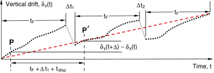
P P tF + t1 + tdisp Vertical drift, y(t) Time, t y(t+ ) − y(t) tF t1 tF tF t2 δ ∆ ∆ ∆ δ δ ∆ ′
Figure 1. Schematic representation for noiseless vertical drift as a
function of time for three images, along with definition of disparity. The dashed line represents the best linear fit.
(This figure is in colour only in the electronic version)
It is noted that (b) and (c) imply that the drift distortion will only be known locally and must be reestimated when a new image is acquired. This ‘incremental’ procedure to determine drift distortion correction requires that corrections be made throughout the experimental process, and is in contrast with spatial distortion, which is determined during the calibration phase and does not require re-estimation during the post-calibration phase of an experiment.
Preliminary experiments and comparison of experimental observations to model predictions clearly indicate that the global model cannot adequately represent experimental observations whereas both the local model predictions are in good agreement with experimental measurements. In the following sections, only the two local models will be discussed in more detail.
2.1.2. Time-based local model. The drift distortion function
is expressed as follows:
Ddr(t )= [δx(t ), δy(t )], units in pixels, (4)
where t is given in equation (3) for a point of interest in the image (x, y).
Consider an object point P located at a position (x, y) in the image plane at timet. At time t + ", the image of the
object point is located at a new position, P′, due to drift.
The difference in positions for the same object point is the disparity, dispdr, and can be written in the form
dispdr= Ddr(t+ ") − Ddr(t ), (5)
with
t= xtD+ ytR
"= tF+ "tn+ tdisp
tdisp= [δx(t+ ") − δx(t )]tD+ [δy(t+ ") − δy(t )]tR,
where "tnis the delay time between one image scan and the
next image scan. Figure1shows a schematic of the process mathematically described by equations (4) and (5), with the experimentally observed shift between images clearly visible since the drift for position (W–1, H–1) is not similar to the drift for position (0, 0) in the next image.
From the drift evolution shown in figure 1, different functional forms can be assumed to represent the local drift. Figure1shows an estimated linear fit to the drift data for three images. The linear fit will smooth regions with high gradients in drift, especially those positions where step changes may occur during the image acquisition process.
To determine the fitting parameters for the assumed form of the drift distortion function, two consecutive images are taken at each step in the experiment. Assuming that only drift occurs between the two images in each consecutive image pair, the drift velocity, vdr(t ), at each position is determined by the
disparity in each pair divided by the time increments:
vdr(t+ "/2) = {[δx(t+ ") − δx(t )]/",
(6) [δy(t+ ") − δy(t )]/"},
where " is defined for pixel (x, y) in equation (5) and the disparity values are obtained in the sensor plane.
Advantages of the time-based approach are its direct relationship with the actual scanning process and the relative simplicity of the data-fitting process for time-streamed disparity data. Disadvantages are as follows: first, there are gaps in the time history due both to the repositioning of the electron beam after each row scan and to the time delay between acquisitions of images. Second, the drift data in actual experiments exhibit step changes in magnitude during the time gaps, resulting in difficulties in extracting accurate results near these positions. Third, finite-sized subsets in the image matching process will introduce averaging effects across the scanned rows, introducing errors in the time-based approach.
2.1.3. Hybrid spatial–temporal (HST) local model. As shown in equations (3)–(5), the drift function can be written in terms of spatial variables, the fixed position (X, Y ). The elapsed time during the whole imaging process for calibration can be written as
t = XtD+ Y tR+ (n − 1)(tF+ "tn), n= 1, 2, . . . , N,
(7) whereN is the total number of images for the drift function
estimation.
In this form, one can write Ddr(X, Y ) as the total drift
function and dispdr(X, Y )as the disparity. The overall imaging process for the HST model is as follows:
• A specimen is patterned so that the SEM images are appropriate for image correlation.
• A sequence of image pairs is acquired. They are numbered as (1, 2), (3, 4), . . . , (n − 1, n) . . . , (N − 1, N), where drift occurs between image n − 1 and n in an image
pair.
• Between the acquisition of each image pair, rigid body motions are applied (these will be used to quantify the spatial distortion field).
• For each image pair, 2D-DIC is performed5to determine
the drift disparity, dispdr(X, Y ), for each fixed position
(X, Y )in the sensor plane.
• A B-spline function is used to obtain a least-squares best fit surface to the components of dispdr(X, Y ) for each
image pair.
• With known values for tD, tRand tF, along with recorded
values for "tn between each image, equation (7) can
be used to determine the elapsed time associated with
5 When using spatially based drift correction, the subset size should be as
small as possible without introducing non-uniqueness in the matching process, thereby minimizing local averaging.
position (X, Y ) in each image. Using equation (6), the velocity of drift for each position, vdr(X, Y; t + "/2), can
be estimated using a central finite difference form. • At each position (X, Y ), vdr(X, Y; t) is fitted with a
B-spline function in time.
• Using the initial condition Ddr(0, 0) = (0, 0) at t = 0, the B-spline approximation for vdr(X, Y; t) can be integrated
over time to determine the drift for each position (X, Y ) in thenth image6, D
dr,n(X, Y ), n= 1, 3, . . . , N − 1.
• Ddr,n(X, Y ) is used to correct images n = 1, 3, . . . ,
N− 1 for the drift distortion.
Mathematically, the determination of the time-dependent drift function for each fixed position (X, Y ) is obtained via minimization of the following functional:
#= N ! n=1 " "vdr(X, Y; tn)− vfitdr(X, Y; aj, tn) " "2, (8)
where aj are the parameters to be fitted and tnis the elapsed
time associated with each drift disparity at the integer pixel position (X, Y ). To obtain the total drift function at each position, Ddr(X, Y; t) = # t 0 $vfit dr(X, Y, aj, t ) % dt, where Ddr(0, 0; t = 0) = 0. (9)
Once the drift distortion is known as a function of time for each pixel position in each image, this field is fitted by a piecewise B-spline to provide a functional form for each image, Ddr,n(x, y), where (x, y) is any real-valued position
in the image.
The HST model described above offers one major advantage: the spatial description of drift within each image minimizes the effects of time gaps on local estimates of the drift function.
2.2. Spatially varying distortions
In simple lens systems, such as those used in a digital camera, spatially varying distortion or spatial distortion (aka image distortion) is a well-known problem. The commonly used method for modelling such imaging systems assumes that the distortions are not a function of time. Classical models used to estimate the spatial distortions are parametric in nature [38]; typical model forms include radial distortion, decentring distortion, prismatic distortion and tangential distortion.
Since the SEM imaging process is based upon the interaction between atoms of the observed specimen and an electron beam, as well as scanning and focusing processes that employ electromagnetic principles to perform the required functions, the pre-specified classical distortions are likely to be ineffective in quantifying arbitrary aberrations or unknown (but deterministic) distortions in a complex imaging system.
6 For the initial image pair, variations in disparity across the image require a
piecewise integration over the disparity field between (0, 0) and (X, Y ) so that the drift at any position (X, Y ) can be determined. A less accurate approach would be to integrate the estimated dispdr(X, Y; t) from t = 0 to the time
corresponding to (X, Y ).
Correlate consecutive images in pair to obtain
drift disparity maps,
dispdr,n(X,Y), n =
1,3,…,N−1.
Determine drift velocity at a finite number of
pixel positions,
vdr,n(X,Y;t+∆/2). Fit 1D
B-spline to time-based data at each position.
Integrate B-spline fit at each location to determine Ddr,n(X,Y).
Correct each position for drift.
Correlate images between pairs to obtain
disparity map for spatial distortion correction, dispsp(x,y).
Perform optimization to determine best fit
spatial distortion function parameters, aj,
and translations, Ti.
Correct each position for spatial distortion by
determined Dsp(x,y).
Fix spatial distortion function. Correct original drifted and distorted positions for
spatial distortion. Fix drift correction
functions. Correct original drifted and distorted positions for
drift distortion.
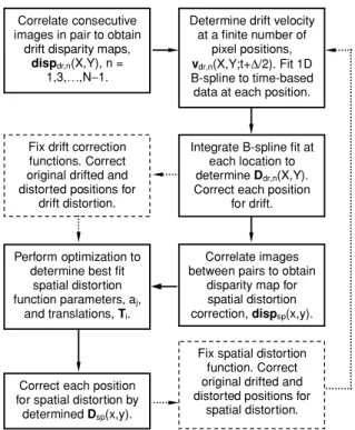
Figure 2. Overall procedure employed for correcting distortion in
an SEM. Relaxation methods are implemented during the process to improve convergence.
To address this issue, non-parametric forms for distortion models are preferred. Two of the earliest such models were proposed by Peuchot [39] and Brandet al [40], where cross targets with known spatial separation are used for the distortion estimation. Since such targets are likely to be difficult to realize at the micro- or nano-scale for the SEM, the work of Schreier
et al using a non-parametric distortion correction approach and
a speckle-patterned calibration target [13] is the most readily adaptable for distortion correction in an SEM, and is employed in previous work [41] as well as in this study.
As outlined by Schreieret al [13], the process uses images acquired during translation along two orthogonal directions and B-splines or other general forms to determine full-field, spatial distortions. Here, it is assumed that the procedures outlined in section2.1.3have been employed to remove drift distortions from all the translated images.
2.3. Overall process for distortion removal
The procedure used in this study to extract drift and spatial distortions is shown as a flow chart in figure 2. The pairs of images are separately correlated throughout the calibration phase and measurement phase to obtain the ‘drift’ at selected pixel positions. The resulting drift disparity fields are used to obtain the drift velocity at selected pixel positions throughout the field of view. Using the velocity field as estimates for the local time derivatives, B-spline fits are obtained for the drift distortion.
After removing the estimated drift distortion from each pixel position, the spatial distortion field and rigid body motions during the calibration phase are determined through an optimization procedure. Relaxation principles are employed
0 1 v( pix els ) 200 400 600 800 x (pixe ls) 200 400 600 y (pixels) -0.5 0 0.5 u( pix els ) 200 400 600 800 x (pixe ls) 200 400 600 800 y (pixels) 0 6 12 18 24 30 0 60 90 120 150 t (minutes)
drift components (pix
els) u v
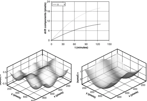
Figure 3. Drift distortion and spatial distortion components for computer simulations with spatial distortion ranging from –0.5 to +1 pixels
and drift ranging up to 20 pixels over 2 h.
during the iteration process to verify that the estimated drift and spatial distortion fields are converged7.
3. Numerical simulations
Consistent with actual experimental conditions, simulations are performed for both the calibration phase and also the measurement phase8. The image correlation process is not
simulated. Both drift and spatial distortion functions are assumed to have pre-defined forms. Using these functional forms, the distorted positions of a finite number of locations, (x, y)k, are determined for each image n. The process is
repeatedN times, so that the distorted positions (x, y)kn, k=
1, 2, . . . , K, n = 1, 2, . . . , N, are determined9. These data
form the basis for the simulation process, with the long-term goal of demonstrating the accuracy and robustness of the approach for SEM image analysis.
3.1. Simulation for the calibration
With "t = 120 s, tD = 10−4s, tR = 1.071 × 10⁻²s and
an imaging array size of 1024 × 884, the positions of image points at 30 specific times (corresponding to 15 image
7 SEM images and the corresponding disparity maps have considerable
electronic and measurement noise. Thus, the HST local drift correction model should employ a reduced order for the B-spline fit to the disparity data so that smoothing of the data is performed during the fitting process to minimize oscillations in the estimated velocity field.
8 The procedure whereby the drift distortion is computed separately for the
calibration and measurement phases is used in practice to minimize the effects of specimen shifts during the initial loading process. However, in principle the process can be continuous.
9 In practice, 7–11 pairs of images are acquired during the calibration phase;
the only requirement is that several translations in two orthogonal directions be performed. The number of pairs of images during the measurement phase will vary with the number of strain increments; for better estimation of the B-spline function at least seven pairs of images should be acquired.
pairs in an experiment) are generated over a total time of 128 min. Between each image pair, the effect of a cross-shaped translation is included in the position of each point. To distort the position of each image point, the drift distortion function Ddr(t ) is assumed to have a quadratic form. The spatial distortion function is assumed to have the form of a combination of cosine wave and a quadratic surface. Figure3
shows the drift and spatial distortion functions. Thus, with the inclusion of random error, the distorted positions of an image point (x, y) in imagen are written as
P′(x, y; t) = P(x, y; t) + Ddr(x(t ), y(t ))
+ Dsp(x, y)+ G(x(t), y(t)), (10)
where G(x, y) is a Gaussian error function with mean value
0 and a pre-defined standard deviation, varying with time and
by equation (3) spatial position (x, y).
Instead of performing correlation to extract the disparity maps, a total of 150 × 120 = 18 000 distorted positions with a spacing of 5 pixels and a ‘beginning’ image position located at (101, 101) are calculated using equation (10) with known vectors on the right-hand side.
To obtain the drift component numerically, all 15 drift disparity maps are computed at each pixel location and equations (6)–(10) are applied to extract Ddr(x, y). Figure4
shows a direct comparison between the computed and the input drift at position (511, 441), where Du and Dv are the differences between the computed and input drift for the horizontal and vertical displacement components, respectively. Figure 5 shows the spatial distribution for the difference between the computed and the input vertical drift for the image acquired att = 36 min.
After correction to remove the effects of drift, the disparity maps are obtained by subtracting the positions of points in the reference image, image 1, from the positions of matching
(a) (b) 0 3 6 9 12 0 30 60 90 120 150 0 30 60 90 120 150 t (minutes) u (pix els) -0.02 -0.01 0.00 0.01 0.02 Du (pix els) input computed difference 0 6 12 18 24 t (minutes) v (pix els) -0.02 -0.01 0.00 0.01 0.02 Dv (pix els) input computed difference 0 3 6 9 12 t (minutes) u (pix els) -0.02 -0.01 0.00 0.01 0.02 Du (pix els) input computed difference 0 6 12 18 24 t (minutes) v (pix els) -0.02 -0.01 0.00 0.01 0.02 Dv (pix els) input computed difference 0 30 60 90 120 150 0 30 60 90 120 150
Figure 4. Comparison of the computed and the input drift at pixel (511, 441) throughout the calibration process: (a) without Gaussian noise
and (b) with a Gaussian noise range of ±0.1 pixels added to the measurements.
Figure 5. Spatial distribution of the difference between computed
and input vertical drift for the image acquired att = 36 min.
points in all other odd-numbered images. The resulting disparity maps have the form
dispsp(x, y)= Dsp(x+ u, y + v) − Dsp(x, y)+ G(x, y), (11) -0.02 0 0.02 Du (p ix els ) 200 300 400 500 600 700 800 900 x (pixe ls) 200 300 400 500 600 700 y (p ixels) -0.02 0 0.02 Dv (p ix els ) 200 300 400 500 600 700 800 900 x (pixe ls) 200 300 400 500 600 700 y (pixels)
Figure 6. Residual difference between the computed and the input distortion. Gaussian noise of ±0.1 pixels applied to input data.
Residuals are less than ±0.02 pixels throughout the field.
where (u, v) is the orthogonal rigid body motion of other images relative to image 1.
By incorporating the computed disparity maps into equation (10), the procedure described in [13] is employed to perform least-squares bundle-adjustment optimization and determine all translations and all parameters in the spatial distortion function. Figure6shows the difference between the computed and the input spatial distortion components in the horizontal (Du) and vertical (Dv) directions, respectively.
As a final check on the accuracy of the drift and spatial distortion correction method, the residual strain fields (with and without Gaussian noise in the displacement values) are computed for all the images within the calibration phase. Without Gaussian noise in the displacement components, the computed strains are less than 1 microstrain throughout the entire sequence. With Gaussian noise having a standard deviation ≈0.025 pixels in each displacement component, all strains have anaverage strain between ±60 microstrain and a
3.2. Discussion
The simulations assumed a total drift of 10–20 pixels over 2 h. Thus, between images in the sequence, the drift is relatively small and the local drift velocities can have considerable oscillation due to electronic noise. Even so, the simulations confirmed that the method proposed will give good overall accuracy, even in the presence of substantial Gaussian noise in the measurements, when combining both drift and spatial distortion corrections.
Since the drift is relatively small between images, it may appear that one can simply ignore this phenomenon. However, our simulations indicate that ignoring or incorrectly estimating drift distortion will introduce substantial errors in the spatial distortion correction that can increase residual strain errors; deviations of the order of 0.001 were observed in this study when incorrectly estimating drift distortion.
4. Experiment validation for calibration and strain measurement
4.1. Experimental setup
Consistent with results obtained in the previous sections, all SEM imagings in this paper are performed using an FEI Quanta-200 SEM in high vacuum mode. For the electron beam, (a) the accelerating voltage is 30 kV, (b) beam spot size is 3, (c) tD= 10−4s, (d) tR= 1.071 × 10⁻²s. The CCD sensor
array has a size of 1024 × 884. These data correspond to tF=
94.67 s. All images are obtained using the BSE detector with a working distance of 14.3 mm. For validation purposes, a magnification of 200× is used, which corresponds to ≈1.25 µm per pixel. The intensity value is stored in 8 bit format in the file.
To apply a micro-scale pattern to the specimen, the procedure described in previous publications [42–46] is used. For comparison to the vision-based measurements, a single strain gauge is aligned with the loading direction. All experiments are performed with the specimen installed in a tensile loading frame and mounted inside the SEM chamber.
4.2. Experiments
The first experiment corresponds to the calibration phase and requires a series of translations in two orthogonal directions performed manually via external motion controls. The second experiment adds a series of strained images that correspond to the measurement phase; uniaxial loading is performed in load control using a Labview control and data acquisition program. After completing each experiment and acquiring all images, the disparity maps are obtained by 2D-DIC using a specially modified version of commercial software VIC2D [14]. All correlations are performed using a 43 × 43 subset size and spacing between subset centres of 5 pixels, the first subset centre is at (101, 101). Thus, all disparity maps contain 18 000 points.
The procedures outlined in figure 2 are employed to determine the drift and spatial distortion functions. To obtain strain fields from the corrected displacement data, local quadratic fits to the displacement components are performed10.
10In this case, the spatial resolution is governed by the subset size. An
estimate for the spatial resolution is ≈25 pixels.
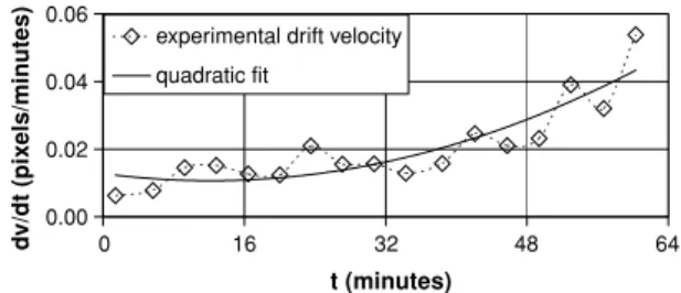
0.00 0.02 0.04 0.06 0 16 32 48 64 t (minutes) dv /d t (p ix el s/ m in u te s)
experimental drift velocity quadratic fit
Figure 7. Measured drift velocity as a function of time at a fixed
pixel location (236, 211) during the calibration phase along with quadratic fit. Data shown are typical of all locations throughout the field.
4.3. Calibration phase—drift and spatial distortion removal
A cross-shaped motion path is performed with 16 motions. Before beginning the motion sequence, two consecutive images are acquired as ‘references’, resulting in a total of 17 pairs of images for calibration.
Figure 7 shows the measured drift velocity in the
y-direction (dv/dt) at location (236, 211), along with the best-fit quadratic function. Though oscillations are clearly present (noise is of the order of ±0.02 pixels), they are small and only visible due to the relatively small drift velocity of 0.01 pixels min–1measured in the SEM at this magnification.
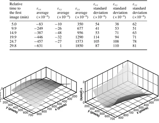
The measured spatial distortion functions are presented in figure8. Here, it is clear that the spatial distortions are much larger than the expected drift distortions, with spatial distortion corrections up to 1 pixel in thex-direction and 2 pixels in the y-direction.
The strain fields are also computed in each of the 16 calibration images. Results indicate that
• the uncorrected εxx, εyy and εxy have average values
approaching 200 microstrain and a standard deviation of 100 microstrain;
• the drift-corrected εxx, εyy and εxy have average values
between 100 and 200 microstrain and a standard deviation of 80 microstrain;
• the spatial distortion-corrected εxx, εyy and εxy have
average values near 50 microstrain and a standard deviation of 60 microstrain;
• the fully corrected εxx, εyy and εxy have average values
near zero and a standard deviation of 60 microstrain.
4.4. Measurement phase—application of uniaxial tension
After completing the calibration phase, the specimen is subjected to increasing uniaxial loading and images are acquired at six different load levels. To minimize the potential for unwanted image motion, after increasing loading on the specimen each time, a hold time of 30 s is maintained prior to acquiring additional images.
To obtain the additional drift components that accumulate during the strain portion of the experiment, the procedures outlined in section 2.1.3 are employed to extract the drift corrections during the loading sequence. Both the spatial distortion and the new local drift functions are used to correct all spatial positions during the loading process. The disparity maps are acquired across corrected odd-numbered images to determine the residual deformation field.
Table 1. Strain data obtained using fully corrected SEM images acquired at seven times during the uniaxial tension loading process.
Relative εxx εxy εyy
time to εxx εxy εyy standard standard standard
the first average average average deviation deviation deviation image (min) (×10−6) (×10−6) (×10−6) (×10−6) (×10−6) (×10−6) 5.0 −83 −10 350 54 38 62 9.9 −249 −26 677 41 53 51 14.9 −387 −48 956 53 71 63 19.9 −446 −32 1290 114 94 71 24.7 −457 −27 1573 105 108 78 29.8 −631 1 1850 87 110 81 -1 0 u( p ix e ls ) 200 300 400 500 600 700 800 900 x (pixe ls) 200 300 400 500 600 700 y (pixels) 0 1 2 v( p ix e ls ) 200 300 400 500 600 700 800 900 x (pixe ls) 200 300 400 500 600 700 y (pixels)
Figure 8. Measured spatial distortion fields. Note the larger gradients in the vertical distortion field.
0 50 100 150
-1000 0 1000 2000 3000
Axial stress vs measured xx and yy (x10 )
Stress (MP a) uncorrected drift corrected fully-corrected uncorrected drift corrected fully-corrected stain gage xx yy xx xx yy yy yy Load xx yy -6
Figure 9. Uniaxial stress versus axial strain and transverse strain for
uncorrected, drift-corrected and fully corrected image correlation data.
Table1presents a summary of the average data across the field, along with estimates for the variability of each strain component. The data in table1indicate that the shear strain is nearly zero throughout the experiment and the standard deviation within the field is less than 114 microstrain for all components.
Figure9presents the average strain data for εxx(transverse
to loading direction) and εyy (along loading direction) at
all loading levels, along with a direct comparison to the independently measured εyy data via a strain gauge. As
shown in figure 9, the average data from the strain gauge and our fully corrected data are in excellent agreement, confirming that Young’s modulus obtained from the strain
gauge measurements and the fully corrected data are nearly the same, 70 GPa. This value is consistent with a wide range of literature values for aluminium alloys.
Also shown in figure9are the strain values that would be predicted using (a) no corrections and (b) drift correction only. It is clear that fully corrected images are necessary for accurate strain estimation so that reasonable estimates can be made for elastic material response.
Finally, since Poisson’s ratio, v, is defined by v = −εxx/εyy, the average measured value using fully corrected
image correlation images is 0.33. This is in good agreement with handbook data, which has a range 0.29 < v < 0.34.
5. Discussion
Algorithms implementing both spatial and drift distortion correction methods have been shown to be effective for removing distortions from SEM images. Thus, the data clearly indicate that basic elastic material properties can be reasonably quantified using digital image correlation with corrected SEM images. Furthermore, even at low magnification, both corrections are essential for accurate measurement of elastic response.
The methods outlined in this work have been extended by the authors to make quantitative, high-accuracy 3D displacement and shape measurements with an SEM [47], the complete development will be the subject of forthcoming papers. For such measurements, the equations of 3D computer vision replace the relatively simple 2D equations given in section 2, and the calibration phase described previously [13] is employed where the specimen is rotated about its eucentric axis to obtain multiple views, and image correlation is employed to locate a dense set of matching positions in
a component. Though no quantitative data are reported, 3D profile results obtained by the authors using stereo images obtained in the FEI Quanta 200 SEM are encouraging and provide confidence that, when completed, the method will be both accurate and robust in such applications.
6. Concluding remarks
The novel method outlined in this work relies on a combination ofa priori drift and spatial distortion correction so that accurate
elastic and elastic–plastic deformation measurements can be obtained using SEM images; both corrections are essential to obtain accurate deformation measurements throughout the field of view.
In sharp contrast to the approach of early SEM measurements, where the investigators simply accepted the accuracy obtainable and successfully performed their studies for important problems amenable to such limitations, this work presents a general approach that successfully extends the range of measurements obtainable in an SEM to the small deformation (elastic) regime so that full elastic–plastic deformation studies can be performed in an SEM.
Simulation results have shown that typical drift processes in an SEM can be adequately reconstructed using local drift velocity measurements. However, if higher gradients in drift are present during the early stages of image acquisition, the simulations also show that image acquisition time should be reduced and additional images need to be acquired during this period for accurate drift reconstruction, a situation that may not be feasible with a given microscope. In practice, image acquisition should be conducted 15–30 min after the first image scan is initiated so that the gradients in drift are reduced to a more manageable level.
Acknowledgments
The support of (a) the National Science Foundation, Dr Oscar Dillon and Dr Kenneth Chong through grant CMS-0201345, (b) Intel and Michael Mello through grant DOCC-22860, (c) the Army Research Laboratory and Dr Adam Rawlett through Cooperative Agreement W911NF0420026 and (d) the Ecole des Mines d’Albi (France) who provided a grant for Nicolas Cornille is gratefully acknowledged. The technical assistance provided by Dana Dunkelberger and Dr Donggao Zhao in the USC Electron Microscopy Center, as well as their financial support of this research, is deeply appreciated.
References
[1] Peters W H and Ranson W F 1982 Digital imaging techniques in experimental stress analysisOpt. Eng. 21 427–32
[2] Mc Neill S R, Sutton M A, Wolters W J, Peters W H and Ranson W F 1983 Determination of displacements using an improved digital correlation methodImage Vis. Comput. 1
1333–9
[3] Chu T C, Ranson W F, Sutton M A and Peters W H 1985 Application of digital image correlation techniques to experimental mechanicsExp. Mech.25 232–44
[4] Sutton M A, Cheng M, Peters W H, Chao Y J and McNeill S R 1986 Application of an optimized digital correlation method to planar deformation analysisImage Vis. Comput. 4 143–53
[5] Khan-Jetter Z L and Chu T C 1990 Three-dimensional displacement measurements using digital image correlation and photogrammic analysisExp. Mech.30 10–6
[6] Luo P F, Chao Y J and Sutton M A 1994 Application of stereo vision to 3D deformation analysis in fracture mechanics
Opt. Eng.33 981–90
[7] Helm J D, McNeill S R and Sutton M A 1996 Improved 3D image correlation for surface displacement measurement
Opt. Eng.35 1911–20
[8] Orteu J J, Garric V and Devy M 1997 Camera calibration for 3-D reconstruction: application to the measure of 3-D deformations on sheet metal partsEuropean Symp. on Lasers, Optics and Vision in Manufacturing (Munich, Germany, June 1997)
[9] Synnergren P and Sjodahl M 1999 A stereoscopic digital speckle photography system for 3D displacement field measurementsOpt. Lasers Eng.31 425–43
[10] Galanulis K and Hofmann A 1999 Determination of forming limit diagrams using an optical measurement system7th Int. Conf. Sheet Metal (Erlangen, Germany, September 1999)
pp 245–52
[11] Sutton M A, McNeill S R, Helm J D and Schreier H W 2000 Computer vision applied to shape and deformation measurementInt. Conf. on Trends in Optical Nondestructive Testing and Inspection (Lugano, Switzerland, May 2000) pp 571–89
[12] Garcia D 2001 Mesure de formes et de champs de d´eplacements tridimensionnels par st´er´eo-corr´elation d’imagesPhD Thesis Institut National Polytechnique de
Toulouse, France
[13] Schreier H W, Garcia D and Sutton M A 2004 Advances in light microscope stereo visionExp. Mech. 44 278–88
[14] VIC-2D and VIC-3D, Correlated Solutions Inc., West Columbia, SC,www.correlatedsolutions.com
[15] Sutton M A, Chae T L, Turner J L and Bruck H A 1990 Development of computer vision methodology for the analysis of surface deformations in magnified images
MiCon 90: Advances in Video Technology for Micro-structural Control (ASTM STP vol 1094)
ed G F Van Der Voort (West Conshohocken, PA: American Society for Testing and Materials) pp 109–32
[16] Mazza E, Danuser G and Dual J 1996 Light optical measurements in microbars with nanometer resolution
Microsyst. Technol. 2 83–91
[17] Mitchell H L, Kniest H T and Won-Jin O 1999 Digital photogrammetry and microscope photographs
Photogramm. Rec.16 695–704
[18] Beyer H A 1992 Accurate calibration of CCD-camerasInt. Conf. on Computer Vision and Pattern Recognition (CVPR’92) (Champaign-Urbana, IL, USA, June 1992)
pp 96–101
[19] Weng J, Cohen P and Herniou M 1992 Camera calibration with distortion models and accuracy evaluationIEEE Trans. Pattern Anal. Mach. Intell.14 965–80
[20] Joy D C 1991 The theory and practice of high-resolution scanning electron microscopyUltramicroscopy 37 216–33
[21] Joy D C, Ko Y-U and Hwu J J 2000 Metrics of resolution and performance for CD-SEMsProc. SPIE 3998 108–114
[22] MeX software; Alicona Imaging;www.alicona.com
[23] SAMx; 3D TOPx package;www.samx.com
[24] Hemmleb M, Albertz J, Schubert M, Gleichmann A and K J M 1996 Digital microphotogrammetry with the scanning electron microscopeInt. Society for Photogrammetry and Remote Sensing
[25] Lacey A J, Thacker N A and Yates R B 1996 Surface approximation from industrial SEM imagesBritish Machine Vision Conf. (BMVC’96) pp 725–34
[26] Agrawal M, Harwood D, Duraiswami R, Davis L and Luther P 2000 Three-dimensional ultrastructure from transmission electron microscope tilt series2nd Indian Conf. on Vision, Graphics and Image Processing (ICVGIP 2000)
[27] Vignon F, Le Besnerais G, Boivin D, Pouchou J L and Quan L 2001 3D reconstruction from scanning electron microscopy using stereovision and self-calibrationPhysics in Signal and Image Processing (Marseille, France, June 2001)
[28] Sinram O, Ritter M, Kleindiek S, Schertel A, Hohenberg H and Albertz J 2002 Calibration of an SEM, using a nano positioning tilting table and a microscopic calibration pyramidISPRS Commission V Symp. (Corfu, Greece)
pp 210–5
[29] Doumalin P 2000 Microextensom´etrie locale par corr´elation d’images num´eriquesPhD Thesis Ecole Polytechnique
[30] Hemmleb M and Albertz J 2000 Microphotography—the photogrammetric determination of friction surfacesIAPRS XXXIII (Amsterdam, The Netherlands)
[31] Lee H S, Shin G H and Park H D 2003 Digital surface modeling for assessment of weathering rate of weathered rock in stone monumentsInt. Archives of the
Photogrammetry, Remote Sensing and Spatial Information Sciences (Ancona, Italy, July 2003)
[32] Dally J W and Read D T 1993 Scanning moir´e at high magnification using optical methodsExp. Mech.33 110–6
[33] Dally J W and Read D T 1993 Scanning moir´e at high magnification using electron beamExp. Mech.33 270–7
[34] Berger J R, Drexler E S and Read D T 1998 Error analysis and thermal expansion measurement with electron-beam moir´e
Exp. Mech.38 167–71
[35] Zhang Z Y 1998 A new multistage approach to motion and structure estimation by gradually enforcing geometric constraintsAsian Conf. on Computer Vision (ACCV’98) (Hong Kong, China, January 1998) pp 567–74
[36] Ravn O, Andersen N A and Sorensen A T 1993
Auto-calibration in automation systems using vision3rd Int. Symp. on Experimental Robotics (ISER’93) (Kyoto, Japan, October 1993) pp 206–18
[37] Lavest J M, Viala M and Dhome M 1998 Do we really need an accurate calibration pattern to achieve a reliable camera calibration?5th European Conf. on Computer Vision (ECCV’98) (Freiburg, Germany, June 1998) pp 158–74
[38] Brown D C 1971 Lens distortion for close-range photogrammetryPhotometric Eng. 37 855–66
[39] Peuchot B 1993 Camera virtual equivalent model 0.01 pixel detectorComput. Med. Imaging Graph.
17 289–94
[40] Brand R, Mohr P and Bobet P 1994 Distorsions optiques: corrections dans un mod´ele projectif9th Congress AFCET, Reconnaissances des Formes et Intelligence Articielle (RFIA’94) (Paris, France, January 1994) pp 87–98
[41] Cornille N 2005 Accurate 3D shape and displacement measurement using a scanning electron microscope,
PhD Thesis Ecole des Mines d’Albi (France)/University of South Carolina
[42] Collette S Aet al 2004 Development of patterns for
nanoscale strain measurements: I. Fabrication of imprinted Au webs for polymeric materialsNanotechnology 15 1812–7
[43] Scrivens W A, Luo Y, Sutton M A, Collette S A, Myrick M L, Miney P, Colavita P E, Reynolds A P and Li X D
Development of patterns for digital image correlation measurements at reduced length scalesExp. Mech.
(at press)
[44] Sutton M A, Zhao W, McNeill S R, Helm J D, Riddell W T and Piascik R S 1999 Local crack closure measurements: development and application of a measurement system using computer vision and a far-field microscope (ASTM STP 1343 on Crack Closure) ed K Smith and J McDowell (West Conshohocken, PA: American Society for Testing and Materials) pp 145–56
[45] Riddell W T, Piascik R S, Sutton M A, Zhao W, McNeill S R and Helm J D 1999 Determining fatigue crack opening loads from near-crack-tip measurements (ASTM STP 1343 on Crack Closure) ed K Smith and J McDowell (West Conshohocken, PA: American Society for Testing and Materials) pp 157–74
[46] Cornille N, Schreier H W, Garcia D, Sutton M A, McNeill S R and Orteu J J 2004 Gridless calibration of distorted visual sensorsColl. Photom´echanique (Albi, France, May 2004)