La nouvelle physique dans le système des mésons B

Université de Montréal

La nouvelle physique dans le système des mésons B

par Philippe Hamel

Département de physique Faculté des arts et des sciences

Mémoire présenté à la Faculté des études supérieures en vue de l’obtention du grade de Maître ès sciellces (M.Sc.)

en physique

avril, 2006

3

n

u9/

o

a

Ô

Université

de Montréal

Direction des bibliothèques

AVIS

L’auteur a autorisé l’Université de Montréal à reproduire et diffuser, en totalité ou en partie, par quelque moyen que ce soit et sur quelque support que ce soit, et exclusivement à des fins non lucratives d’enseignement et de recherche, des copies de ce mémoire ou de cette thèse.

L’auteur et les coauteurs le cas échéant conservent la propriété du droit d’auteur et des droits moraux qui protègent ce document. Ni la thèse ou le mémoire, ni des extraits substantiels de ce document, ne doivent être imprimés ou autrement reproduits sans l’autorisation de l’auteur.

Afin de se conformer à la Loi canadienne sur la protection des renséignements personnels, quelques formulaires secondaires, coordonnées ou signatures intégrées au texte ont pu être enlevés de ce document. Rien que cela ait pu affecter la pagination, il n’y a aucun contenu manquant. NOTICE

The author of this thesis or dissertation has granted a nonexciusive license allowing Université de Montréal to reproduce and publish the document, in part or in whole, and in any format, solely for noncommercial educational and research purposes.

The author and co-authors if applicable retain Copyright ownership and moral rights in this document. Neither the whole thesïs or dissertation, nor substantial extracts from it, may be printed or otherwise reproduced without the author’s permission.

In compliance with the Canadian Privacy Act some supporting forms, contact

information or signatures may have been removed from the document. While this may affect the document page count, it does not represent any loss of

faculté des études supérieures

Ce mémoire intitulé:

La nouvelle physique dans le système des mésons B

présenté par: Philippe Hamel

a été évalué par un jury composé des personnes suivantes: Manu Paranjape président-rapporteur David London directeur de recherche Georges Azuelos membre du jury

RÉSUMÉ

Ce mémoire a pour but d’étudier la phénoménologie des mésons B et de résoudre certailles divergences existantes entre l’expérience et la théorie en supposant de la physique au-delà du modèle standard (MS). Pour ce faire, o y étudie en particu lier les désintégrations B —+ ‘îrK et B —+ pK*. Le mémoire inclut une introduction théorique et deux articles. La partie théorique décrit la violation CP dans le MS ainsi que la phénoménologie des mésons B. Le premier article étudie la désiilté gration B —* _{irK par ue méthode numérique. Nous avons démontré qu’il y a une} divergence entre les prédictions théoriqiles et les mesures expérimentales. Pollr ré soudre le problème, nous avons proposé différents opérateurs de nouvelle physique. Nous avons trouvé une classe d’opérateurs permettant d’expliquer les mesures. Dans le dellxième article, nous avons calculé les effets qu’auraient ces opérateurs dans la désintégration B —+ pK*. Nous avons trouvé que seulement les opérateurs

f?R

b7Rsd7Rd et fL b7Lsd7Ld peuvent résoudre à la fois le casse-tête de B -4 irK et le problème de polarisation dans B —+ pK*.

Mots clés: phénoménologie, mésons B, violation CP, nouvelle phy sique.

The goal of this thesis is to study the phenomenology of B mesons ami to solve some discrepancies that exist between experiment and theory by adding physics beyond the standard model. In order do to that, we study, in particular, the decays B —+ rrK and B —+ pK*. The thesis includes a theoretical introduction and two articles. The theoretical part describes CP violation in the standard model and B-meson phenomenology. The first article studies the decay B —* 7rK by doing a numerical fit. We show that there is a discrepancy between theoretical predictions and experimental results. In order to solve this problem, we test many classes of new-physics operators. We find one class of operators that can explain the experimental data. In the second article, we calculate the effects of those operators in the B —+ pK* system. We find that only operators of the type

f

6’yRsd7Rd and

fL

b7Lsd7Ld can explain both the B — irK puzzle and the polarization problem in B —+ pK*.

TABLE DES MATIÈRES

RÉSUMÉ .. iii

ABSTRACT iv

TABLE DES MATIÈRES y

LISTE DES TABLEAUX vii

LISTE DES FIGURES viii

LISTE DES SIGLES ix

REMERCIEMENTS x

INTRODUCTION 1

CHAPITRE 1 : LA VIOLATION CP DANS LE MODÈLE STAN

DARD 3

1.1 Symétries 3

1.2 Le système des kaons neutres 4

1.3 Matrice CKM 7

1.4 Phases faibles et fortes 9

CHAPITRE 2: PHÉNOMÉNOLOGIE DES MÉSONS B 11

2.1 Diagrammes de Feynman 11

2.2 Opérateurs 14

2.3 Mélange B° - 16

2.4 Observables 17

vi CHAPITRE 3 : LE CASSE-TÊTE DE B - 7UK ET LA

PHYSIQUE

CHAPITRE 4: LES ÉTATS DE POLARISATION DE LA NOUVELLE PHYSIQUE

4.1 Introduction

4.2 B —* pK* Staildard Model Predictions 4.3 B — irK Decays 4.4 3 —+ pKt New-Physics Contributions 4.5 B—*ç5K 4.6 Conclusions NOUVELLE B — _{pK* ET} 31 33 34 41 44 51 52 CONCLUSION 55 BIBLIOGRAPHIE 57.

LISTE DES TABLEAUX

1.1 La composition en quarks de quelques mésons 5 1.2 Temps de vie des deux types de kaons neutres 5 3.1 Branching ratios, direct CP asymmetries and mixing-induced

CP asymmetry Ajndjr (if applicable) for the four B — nK decay

modes 24

4.1 Branching ratios and polarization fractions for the two B+ pK* decays. Data cornes from Ref. [38j; averages are taken from Ref. [39] 40 4.2 Contributions to the polarization states of B —+ pOK*+ from the

various NP operators. Operators which are not shown do not contri bute. The various Z’s and X’s are defined analogously to Eqs. (4.3$)

and (4.44). We take j 49

4.3 Contributions to the polarization states of 3 p+K*O from the various NP operators. Operators which are not shown do not contri bute. The various Z’s and X’s are defined analogously to Eqs. (4.3$)

1.1 Exemple de triangle unitaire 9

2.1 Arbre favorisé par la couleur (T’) 12

2.2 Arbre supprimé par la couleur (G’) 12

2.3 Pingouin gluonique (P’) 13

2.4 Pingouin électrofaible (P,) 14

2.5 Pingouin électrofaible supprimé par la couleur (P,) 14

LISTE DES SIGLES

A Axial

C Charge

CKM Cabibbo, Kobayashi et Maskawa CP Charge-Parité

MS Modèle Staildard NP Nouvelle Physique

P Parité

Je tiens à remercier tout d’abord mon directeur de recherche David London. J’ai toujours apprécié sa méthode pédagogique. Il a été un excellent guide pendant les deux dernières années. Son expérience et sa grande connaissance du domaine lui ont permis de nous diriger, moi et les co-auteurs, pendant l’élaboration des articles. Je tiens également à remercier tous les co-auteurs des articles. J’ai apprécié travailler avec eux. Les nombreuses discussions que nous avons eues ont été très éclairantes.

Un gros merci aussi aux «bananes théoriques volantes». Ces créatures sympa thiques qui vivent au V-207 ont su garder une belle ambiance de travail. Grâce à elles, j’ai pu résoudre d’innombrables petits problèmes. J’ai beaucoup apprécié travailler avec vous!

Je veux aussi remercier les habitués de la Planck. Vous avez été d’une grande aide pendant les années de bacc et de maîtrise. Je n’aurais probablement pas réalisé ce mémoire sans votre présence. C’est grâce à votre sens de l’humour que j’ai pu garder (une partie de) ma sanité d’esprit pendant ces cinq années d’étude en physique.

Enfin, un merci très spécial à Ariane. Elle m’a supporté, dans tous les sens du termes, pendant la dernière année. Sans elle, ce mémoire aurait probablement été beaucoup plus pénible à lire.

INTRODUCTION

Le système des mésons B est un sujet encore jeune de la physique des particules. Cela est dû entre autres au fait que les infrastructures expérimentales nécessaires à l’étude de telles particules lourdes ne sont disponibles que depuis quelques années. Depuis, on a construit des « usines à B » telles que Babar, aux tats-Unis, et Belle, au Japon. Ces laboratoires ont pour but premier d’étudier les désintégrations des mésons B. Grâce à de tels projets, nous disposons maintenant de données expérimentales de plus en plus précises pour vérifier la validité du modèle standard (MS). Toutefois, ces données ont encore de grandes incertitudes et il est encore tôt pour en arriver à des conclusions claires. Une étude théorique des résultats actuels peut motiver le besoin d’augmenter la précision de certaines mesures et diriger les expérimentateurs vers de nouvelles pistes.

Ce mémoire a pour but d’étudier la phénoménologie des mésons B et de résoudre certaines divergences entre l’expérience et la théorie grâce à de la physique au-delà du M$. On étudiera en particulier les désintégrations B —+ 7rK et B —+ pK*.

Pour ce faire, le mode de présentation par articles a été choisi. Les deux premiers chapitres formeront un survol des notions importantes à la compréhension des articles présentés. Le premier chapitre traitera principalement de l’aspect théorique de la violation CP dans le M$. Le second portera plutôt sur la phénoménologie spécifique aux mésons B, en particulier des désintégrations à l’étude.

Le troisième chapitre est constitué de l’article intitulé «The B —+ rrK Puzzle

and New Physics». Dans cet article, on étudie les divergences entre le M$ et les résultats expérimentaux grâce à des comparaisons numériques. On y inclut des opérateurs de nouvelle physique (NP) et on vérifie lesquels ajusteraient mieux les résultats. Nous avons trouvé qu’un type particulier d’opérateur permet de résoudre les problèmes dans ce systènie. Ma contribution personnelle à cet article a été de travailler sur un programme, en collaboration avec S. Baek, et d’effectuer les simu lations numériques. Grâce au programme, j’ai pu montrer que le modèle standard ne s’accorde pas avec les résultats expérimentaux. J’ai ensuite ajouté différents

opérateurs de NP à la simulation. Cela nous a permis de trouver le meilleur type d’opérateur pour résoudre la divergence. Mon programme a utilisé la routine de mi nimisation de fonction MINUIT. Par souci de rigueur, nous avons ensuite comparé nos résultats à ceux de D. Suprun, générés par un programme indépendant.

Le quatrième et dernier chapitre inclut un autre article intitulé «Polarization States in B —* pK* and New Physics». Cet article fait suite à celui du troisième chapitre. Nous utilisons le type d’opérateurs obtenus pour le système B — irK afin de résoudre le problème de polarisation dans le système B —+ pK*. On trouve qu’il est possible d’accorder l’expérience à la théorie dans ces deux systèmes grâce à l’ajout de certains opérateurs spécifiques de nouvelle physique. J’ai contribué à cet article dans la discussion et la documentation nécéssaire à la compréhension du sujet traité. J’ai également effectué les calculs présentés dans l’article. Les calculs ont montré que parmi les seize opérateurs trouvés dans le premier article, seulement deux contribuent significativement à la polarisation transversale de B+ p+K*O. Ces deux opérateurs permettraient donc de résoudre à la fois le casse-tête de B —+ nK et le problème de polarisation dans B —+ pK*. Encore une fois par souci de rigueur, ces calculs ont été comparés à ceux d’A. Datta et de S. Baek qui ont été effectués indépendamment.

CHAPITRE 1

LA VIOLATION CP DANS LE MODÈLE STANDARD

Commençons tout d’abord par un bref survol de la violation CP dans le modèle standard (MS). On sait que les symétries sont très importantes en physique. Jusqu’à il y a environ quarante ans, on croyait que la symétrie CP était une symétrie intrinsèque de la nature. La découverte de la violation d’une telle symétrie nous a forcé à revoir notre façon de comprendre la nature. On a dfi faire de nouvelles hypothèses et postuler l’existence de nouvelles particules.

Kobayashi et Maskawa ont proposé d’étendre la matrice de Cabibbo à une troi sième famille de quarks. De cette façon, la nouvelle matrice de mélange des quarks, aujourd’hui appelée matrice CKM pour Cabibbo, Kobayashi et Maskawa, inclut une phase irréductible qui engendre de la violation CP dans l’interaction faible. Cette matrice possède des paramètres que l’on peut déterminer par l’expérimenta tion. Toutefois, quelques-uns de ces paramètres restent à ce jour assez mal connus.

1.1 Symétries

La physique utilise souvent la symétrie afin de simplifier et résoudre des pro blèmes complexes. Souvent, les symétries ne sont pas que de simples approxi mations, mais font partie intégrante du système étudié. Par exemple, le modèle standard actuel est décrit par un ensemble de groupes de symétrie SU(3) 0

SU(2)L 0 U(1)y. Grâce au théorème de Noether, on sait que toute symétrie du système impose une quantité conservée. Par exemple, l’isotropie de l’espace impose la conservation de l’impulsion et l’invariance sous rotation impose la conservation du moment angulaire. Donc, pour bien comprendre le comportement d’un système, il est crucial de connaître ses symétries.

La symétrie de parité P (x —÷ —x) a longtemps été considérée comme une sy

d’inverser l’impulsion (p —+ —p) et de laisser le moment angulaire (et le spin) illva

riant (J — J). Donc, un changement de parité transforme ue particule gauchère

(le spiil dails la direction opposée à l’impulsion) en une particule droitière (le spin aligné avec l’impulsion). On a découvert au cours du dernier siècle que cette symé trie n’est pas tout à fait conservée. En fait, on dit qu’elle est «violée maxirnalement» par la force faible. On peut le voir par le fait que la force faible interagit avec les neutrinos gauchers, mais pas avec les neutrinos droitiers (qui, par conséquent, ne semblent pas interagir avec notre univers).

La symétrie de conjugaison de charge C (qui consiste à changer une particule pour son antiparticule) est elle allssi violée maximalement par la force faible. Si on reprend l’exemple du neutrino gaucher et qu’on applique maintenant une transfor mation de conjugaison de charge, on obtient un anti-neutrino gaucher, qui ne peut interagir par la force faible.

On a donc que P et C sont violées maximalement. On peut se demander quelles symétries sont bel et bien conservées. Qu’en est-il de CP, la transformation qui combine conjugaison de charge et parité? Une transformation CP appliquée à notre fidèle neutrino gaucher le tranforme en anti-neutrino droitier qui peut interagir avec la force faible.

À

priori, la symétrie CF semble être respectée par l’interaction faible, comme pour les autres interactions.

Après la découverte de la violation de P, les physiciens de l’époque se sont rabattus sur la symétrie CF en croyant que celle-ci était une symétrie fondamentale de la nature. Mais la nature n’est jamais aussi simple qu’on le croit. En 1964, ne expérience sur les kaons neutres obtient des résultats déconcertants qui viennent encore une fois révolutionner la physique.

1.2 Le système des kaons neutres

Les mésons K, aussi appelés kaons, sont constitués d’un quark « étrange » s et d’un quark de la première famille (u ou cl). Le système des kaons neutres possède des propriétés très partidillières qui nons ont permis d’observer la brisure de la

5 symétrie CP pour la première fois.

TAB. 1.1 — La composition en quarks de quelques mésons

Méson quarks spin conjugué CP

0 uii—dd 0 7t u 7C ir+ ₀ K° d O K O B° db

o

B O B 0 1 0 p p p ud 1 p K*o _{d 1} K*+ ₁

Puisqu’il y a deux kaons neutres, il y a deux états propres de masses. Ces états de masse sont des combinaisons linéaires des états K° et et ont un temps de vie bien défini. On appelle K,9 (S pour «short-lived») l’état ayant le temps de vie le plus court et KL (L pour «long-lived») celui ayant le temps de vie le plus long.

Les kaons neutres peuvent se désintégrer en deux ou trois pions. On remarque expérimentalement que les désintégrations en deux pions s’effectuent beaucoup plus rapidement que celles en trois pions. Cela est dû au fait que la masse des kaons neutres (494 MeV) est près de la masse de trois pions (3 fois 135 MeV). Les états de masse sont donc tels que I(. se désintègre principalement en deux pions et KL en trois pions. On voit dans le tableau 1.2 que le temps de vie de KL est en fait 600 fois plus grand que celui de K3.

TAB. 1.2 — Temps de vie des deux types de kaons neutres

r8 (0, 8926 ± 0, 0012) X 10° s

Les états propres de CP des kaons neutres sont

K° 1

1 —

K° — 1k(7O — 1kr-o

De plus, on sait que

CP un) = + un)

CF unir) — nrr7r). (1.2)

C’est-à-dire que l’état à deux pions est un état purement CP+, et celui à trois pions est purement CP-.

Si CP est conservé, on sait que les états propres de masses seront les états CP. Il est donc naturel d’associer KL à K_ et K3 à Kcp+. On peut vérifier expérimentalement une telle supposition. On utilise la grande différence de temps de vie afin d’obtenir expérimentalement un faisceau constitué presque exclusivement de KL. En effet, dans un faisceau constitué d’un mélange quelconque de K° et de

Ï,

la composante K3 va naturellement se désintégrer sur un temps très court, et laisser seulement la composante KL. Par ce stratagème, on a pu obtenir un signal très clair que, contrairement aux attentes, la désintégration KL —+ un est possible.

Cela signifie que les états propres de masse KL,s ne correspondent pas aux états

CP. On a donc que

1__2p_)+E))

(1.3)

où = 2, 3 x ïO [4]. Le fait que e soit non-nul est une preuve directe que la

7 L3 Matrice CKM

On sait que les quarks peuvent changer de saveur uniquement par l’interaction faible. Supposons qu’un quark q [antiquark ?‘] interagit avec un 11/ pour se trans former un quark q’ [antiquark

_9.

Dans le calcul de l’amplitude de ce processus, on aura un facteur V [V] qui apparaîtra dans le terme du vertex. Ce facteur est un élément de la matrice de mélange des quarks.

Avant la matrice CKM, on ne connaissait que deux familles de quarks. La matrice de mélange des quarks était donc une matrice unitaire 2 x 2 à coefficients complexes. On peut montrer qu’une telle matrice peut être paramétrisée par un seul angle réel (l’angle de Cabibbo). Une telle matrice n’aurait pas permis de violation CP.

En 1973, Kobayashi et Maskawa porposèrent d’ajouter une famille de quarks aux deux déjà connues dans la matrice de Cabibbo. La matrice de mélange de quarks devient alors une matrice unitaire 3 x à coefficients complexes. On peut montrer qu’une telle matrice peut être paramétrisée par trois angles réels et une phase complexe. Cette phase peut être la source d’une violation CP. Le grand succès de la matrice CKIVI a été de postuler l’existence d’une troisième famille de quarks 10 ans avant la première observation expérimentale d’un quark b. On peut écrire la matrice de mélange de quarks comme

VdVVb V VdV3Vb 4s 4b C12C13 Sl3613 = —812C23 — C12S23S138’ C12C23 — s12s23s13e’ S23l3 . (1.4) S12523 — ci2c23si3e113 —c12s23 — c23c13

Il existe plusieurs paramétrisations de la matrice V. Une des plus utiles est la paramétrisation de Wolfenstein

_t31

Elle fait un développement de chacun des éléments en termes de puissances de X. Celle-ci découle directement de l’éq.(1.4)

en posant ;2 À 0.22, s23 AÀ2 et s13e AÀ3(p —in).

À

l’ordre À3 on a À AÀ3(p—i’rj)

V —À 1 — ‘À2 AÀ2 + 0(À4) (1.5)

AÀ3(1—p—irj) —AÀ2 1

où A, p et i sont des paramètres réels de l’ordre de l’unité. On peut remarquer que

sous cette paramétrisation, seillement Vb et Vd sont complexes à l’ordre À3. On peut donc écrire

Vd V8 Vlibe

V Vd Vcs Vb (1.6)

Vd 4s

L’unitarité de la matrice implique les relations suivantes

V.2=1 j=1,2,3 (1.7)

/jV = O j,k = 1,2,3

j

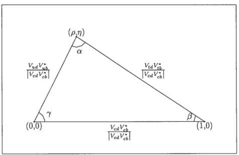
k (1.8)

Les six équations de (1.8) peuvent être représentées de façon géométrique par six triangles à aires égales dans le plan complexe. En particulier l’équation

(1.9)

représentée par le triangle de la figure 1.1 a la particularité d’avoir trois côtés du même ordre de grandeur. On remarque que les angles 7 et /3 du triangle sont les mêmes que dans la matrice CKM de l’équation (1.6) et que c —

/3

9

FIG. 1.1 — Exemple de triangle unitaire. 1.4 Phases faibles et fortes

Considérons un processus qui comporte un seul diagramme de Feynman. L’am plitude de ce processus est donnée par

A = A ee6 (1.10)

où q représente la phase «faible» et c5 représente la phase «forte». La phase forte vient de l’interaction forte, elle est donc invariante sous CP. La phase faible, quant à elle, provient de la matrice de mélange des quarks et change de signe sous CP. L’amplitude de l’anti-processus est donc

CP(A) == (1.11)

On remarque que dans le cas où il y a un seul diagramme en jeu, AI2=2.

V dV*

7cdV

,0)

Considérons maintenant un processus à deux diagrammes. Les amplitudes du pro cessus et de l’anti-processus sont

A — A1

I

e’ e’ + lA2

e2 eZ62

A = Aj e1e1 + A21e2ei62. (1.13)

Donc,

AI2 = lA1 2 + lA2 2 + 2 A11 A21 (cos(i — 2) cos(61 — 62) —sin@i

— 2) sin(6; — 62))

= 12 + lA2 2 + 2 A A21 (cos(i

— 2) cos(61 62)

+sin(q1 — ç2)sin(61 —62)). (1.14)

Ce qui implique que

AI2

2

(1.15) si çb ç et 6 62. C’est ce qu’on appelle la violation CP directe. Elle se manifeste

lorsqu’un processus provient de deux diagrammes ou plus ayant des phases faibles et fortes différentes. On verra au chapitre 2 comment on observe expérimentalement cette asymétrie. On verra également qu’il est possible d’observer la violation CP même s’il n’y a pas de violation directe.

CHAPITRE 2

PHÉNOMÉNOLOGIE DES MÉSONS B

La matrice CKM peut être paramétrisée par quatre constantes réelles. Il est pos sible de contraindre la valeur de ces constantes par l’expérimentation. Les systèmes de mésons légers ne nous permettent pas de mesurer efficacement ces paramètres puisque la violation CP y est plutôt faible. Par contre, dans le système des mésons B on prédit une forte violation CP. Cela est dû au fait que V et V, deux élé ments de la matrice CKM que l’on retrouve dans les désintégrations et le mélange des mésons B, ont des phases faibles importantes. C’est donc un système idéal pour contraindre les paramètres et tester si le modèle est bien valide.

À

ce jour, plusieurs mesures expérimentales sont encore trop incertaines pour arriver à des conclusions claires. Toutefois, on voit déjà apparaître plusieurs indices portant à croire que la description du MS est incomplète. On peut donc émettre des hypothèses sur la nouvelle physiqile (NP) qui pourrait unir expérimentation et théorie. Bien sûr, avant de proposer de nouvelles théories, il est important de bien comprendre ce que le IVIS prédit.

Dans ce mémoire, on se limite à l’étude de B —+ 7TK et B —+ pK*. Ces deux systèmes ont la même composition en quarks. Les diagrammes intervenant dans les différents processus seront donc les mêmes. Tous ces diagrammes auront une désintégration

6

—+ q?j (q = u, d). De plus, si on ajoilte de la NP à un des deux

systèmes, l’autre sera également affecté.

2.1 Diagrammes de Feynman

Premièrement, énumérons les différents diagrammes de Feynman qui intervien dront dans les désintégrations

6

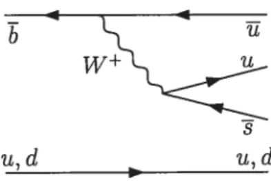
—+ q?j (q = u, U) à l’étude dans ce mémoire.

On a tout d’abord les diagrammes en arbre (figs. 2.1 et 2.2). On dit qe le diagramme C’ est «supprimé par la couleur» car la conservation de la couleur

fIG. 2.1 — Arbre favorisé par la couleur (T’) — b U W+

E

s ud

FIG. 2.2 — Arbre supprimé par la couleur (C’)

impose la couleur des quarks générés par le W dans ce diagramme. En effet, la couleur de ces quarks doit correspondre à la couleur du quark spectateur. Pour le diagramme T’, au contraire, les quarks générés par le W ont le choix de la couleur

(r, b ou g). On peut donc poser naïvement que l’amplitude T’ devrait être

trois fois plus grande que C’. Le facteur CKM de ces diagrammes est VbVUS. Ils possèdent donc une phase faible e7 (éq. 1.6).

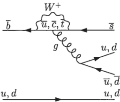
On a ensuite les pingouins gluoniques (fig. 2.3). Il y a trois pingouins gluoniques différents (Pi, P et P) puisqu’il y a trois quarks internes possibles dans la boucle. Chacun de ces termes possède un facteur CKM différent. Cependant, on utilise

13

FIG. 2.3 — Pingouin gluonique (P’)

l’unitarité de la matrice CKM (éq. 1.8) pour mettre en relation ces diagrammes et réécrire l’amplitude avec seulement deux termes. On a donc

P’ = VbVu P + VVcs P + 1’4 P’ V*V P + P (2.1)

où P = P — P et P = P

—

i•

On voit que P possède une phase faible et que P n’en a pas. De plus, on sait que

v*v

ubL8

(2.2)

V

cb cs

Par conséquent, la contribution de P sera beaucoup plus importante que celle de p,ut

Finalement, on a les pingouins électrofaibles (figs 2.4 et 2.5). Comme pour les diagrammes en arbre, on a un diagramme favorisé par la couleur et un supprimé par la couleur. On peut donc poser que P/Pf 3. Dans ces diagrammes, le couplage du Z° au quark q nous donne un terme proportionnel à m. Puisque

m

«

m

«

mt, on peut considérer seulement le diagramme avec un quark t. Dans ce cas, le facteur CKM est Il n’y a donc pas de phase faible pour ces diagrammes.

g

u,d — u,d

FIG. 2.5 — Pingouin électrofaible supprimé par la couleur (P,)

2.2 Opérateurs

L’amplitude totale d’une désintégration B —+

J

peut s’écrire comme

A =

(J

Heff B) (2.3)

OÙ Heff est l’hamiltonien effectif. Celui-ci peut s’écrire comme une combinaison linéaire d’opérateurs représentants les différents diagrammes. L’hamiltonien effectif

u,d

z0,

FIG. 2.4 — Pingouin électrofaible (P)

z0,

u’

15 est donné par

Hef_f [VUbV5(Cl0l + c202)

—

+ lic.. (2.4)

Les c sont les coefficients de Wilson. Les O sont définis comme

01 = (u)V_AQfib)l’_A, 02 (u) VAQub)VÀ,

03 = (b)v_A(?jq)v_A, 04 = (ck)v—A Zq(qc) V—A,

05 = (b)v_A(q)v+A, 06 =

07 = (b)v_A eq(q)v+A, 0 (b)vAZq eq(qa)v+A,

09 = (b)v_Aeq(q)v_A, 010 = (b 7A Zqeq(q) v_A (2.5)

où (?jq’)v+A = 7(1 + 7s)q’ et cv, sont des indices de couleur. Les diagrammes en

arbre sont représentés par les opérateurs 01 et 02, les pingouins gluoniques par 03

à O et les pingouins électrofaibles par 07 à 010.

Même en utilisant l’hamiltonien effectif, les éléments de matrice restent com plexes à calculer. Dans les calculs du chapitre 4, on utilise l’approximation dite «factorisation naïve». Cette dernière nous donne des résultats peu précis, mais nous permet de négliger des effets difficiles à calculer tels que la rediffusion.

Avec la factorisation naïve, on peut séparer les éléments de matrice en deux facteurs. Voici un exemple de calcul pour l’amplitude d’un diagramme en arbre

T+oK+ = (0K VbV*(c + _{)(u)v_A(b)v_A} B) (2.6)

= VlibV8(c1 +

)

K°’

— 75)b B)

KK7(1

—7 O). Ces éléments de matrice peuvent être calculés en utilisant des facteurs de forme. Les différents éléments de matrice utilisés dans ce mémoire sont donnés dans l’annexe du chapitre 4.

2.3 Mélange B°

-Dans le système des mésons neutres, il existe un phénomène de mélange. C’est-à-dire qu’un méson neutre peut se tranformer en son anti-particule. Donc, un B° peut se transformer en et vice-versa. Les diagrammes responsables pour de tels échanges sont les diagrammes en boîte (fig. 2.6).

6

B° W W

U n,t b

f1G. 2.6 — Diagramme de mélange B° —

On remarque que trois quarks et trois anti-quarks sont possibles. Toutefois, l’amplitude du diagramme avec t et domine largement tous les autres. Cela est dû à un facteur proportionnel à m qui apparaît dans le calcul de l’amplitude. On peut donc dire qu’à une bonne approximation, le facteur CKM de ce diagramme est (V14d)2, ce qui donne une phase faible de

Puisqu’on sait que CP n’est pas conservé, les états de masse ne sont pas nécés sairement équivalents aux états propres de CP. On peut définir les états de masse par

BH) = p B0) + q 3°)

BL) = p BD) — q

)

(2.7)

17 définir l’évolution à travers le temps de l’état d’un 3° ou pur par

B0(t)) _{g(t) 3°) +g(t)}

₎

= g(t) 3°) + g(t)

)

(2.8)

g(t) + e_i(mL_t). _(2.9)

Les termes mH,L et FH,L représentent respectivement la masse et la largeur de désintégration des états BH et BL.

Un fait important à remarquer est que

Prob(B°(t)

₎

Prob((t) 3°) (2.10)

C’est ce qu’on appelle la violation CP dans le mélange. On a mesuré expérimenta lement ce phénomène par les désintégrations semi-leptoniques des B neutres. On n’a toujours pas trouvé à ce jour d’asymétrie dans le mélange des mésons B

[61.

On pellt donc écrire comme une phase pure. Si on fait l’approximation que le

diagramme de mélange dominant est la boîte avec deux quarks t, on a que

= e. (2.11)

p

2.4 Observables

Expérimentalement, ce que nous observons est f(X(t) —÷ Y) et f(X(t) —+

Y),

les rapports d’embranchement d’un processus et de son anti-processus. On peut intégrer sur le temps pour obtenir les rapports indépendants du temps F(X —+ Y) et F(X —+

Y).

Dans les processus qui nous intéressent, on peut extraire trois types d’observables.

Il y a tout d’abord le rapport d’embranchement moyen indépendant du temps:

Br(Bf)=3. (2.12)

Cette observable est évidemment indépendante de la violation CP pilisque Br(B —÷

f)=

Br(-+J).

On peut également mesurer l’asymétrie directe indépendante du temps

Adir F(B-f)-F(-J)

= F(B

f)

+ f(

(2.13)

Si ce terme est non-nul, cela implique que l’équation (1.15) est respectée. Toute fois, l’asymétrie directe ne nous donne pas toute l’information sur la brisure de la symétrie pour les mésons neutres. Puisqile les rapports d’embranchement sont intégrés dans le temps, on perd de l’information. Justement, les mésons neutres oscillent entre particule et anti-particule dans le temps. Pour tenir compte de ce fait, on doit considérer les rapports d’embranchement dépendants du temps. Le terme d’asymétrie le plus général est

F(B(t) -*

f)

- F((t)

-*1)

A0p(t) — — — . 2.14

F(B(t) -*

f)

+ F(B(t) -*

f)

Considérons un état final f qui est un état propre de CP (i.e.

_f

=

J).

Donc, par

l’éq. (2.8) et par le fait que

F(X Y) = (Y H X)2 = A(X Y)2, (2.15)

on peut montrer que

1 — 2ImÀ

= + 2

cos(mt)

— + j2 sin(mt)

19

où Am = mH — mL et — —

qA(B—f) —

A(Bf) —e 2.1

On voit par l’éq. (2.13) que C).) Il nous reste le terme $(À) comme obser vable indépendante du temps. C’est ce qu’on appelle l’asymétrie due à l’interférence entre les désintégrations avec et sans mélange ou, plus simplement, asymétrie indi recte

= $(À) = 122. (2.18)

2.5 Polarisation

Une dernière observable est pertinente à notre étude. Dans les systèmes de par ticules vectorielles tels que B —* pK*, les particules finales ont une polarisation. Une particule massive de spin 1 a trois états de polarisation possibles gaucher(—), droitier(+) ou longitudinal(O). Dans les désintégrations B —* VV, les deux parti cules vectorielles doivent avoir la même polarisation puisque les mésons B sont de spin O. Cette polarisation peut être observée expérimentalement. Il est donc pos sible d’obtenir un rapport entre les différentes polarisations finales.

À

cause de la forme (V—A) x (V+A) des opérateurs du M$, la polarisation longitudinale devrait naïvement dominer (éq. 4.6). Toutefois, les résultats expérimentaux des systèmes B —+ pKt et B —* K* ne semblent pas respecter cette prédiction théorique.

LE CASSE-TÊTE DE B - irK ET LA NOUVELLE PHYSIQUE

The

B

—+

zrK Puzzle and

New Physics

[11

$eungwon Baek

a

Alakabha Datta

b,

Philippe Hamel

Denis A. Suprun

C

_{and David London}

a : Physique des Particules, Université de Montréat,

C.P. 6128, suce. centre-mite, Montréat, QC, Canada H3C 3J7 b Department of Physics, University of Toronto,

60 St. George Street, Toronto, ON, Canada M55 1A7 e t Physics Department, Brookhaven National Laboratory,

Abstract

The present B —÷ rrK data is studied in the context of the standard model ($M) and with new physics (NP). We confirm that the SM has difficulties explaining the B —+ rrK measurements. By adopting an effective-lagrangian parametrization of NP effects, we are able to rule out several classes of NP. Our model-independent analysis shows that the B —+ rrK data can be accommodated by NP in the elec

The B-factories BaBar and Belle have measured (most of) the branching ratios and CF asymmetries for the variolls B — r’ir and B —+ irK decays, and these can be used to search for physics beyond the Standard Model (5M). By using fiavor $U(3) symmetry to relate these processes

_[9—’1,

several analyses were able to constrain the SM parameters, and to look for signs of New Physics (NP). The advantage of this approach is that one takes into account a large number of processes. The disadvantage is that one lias to deal with unknown effects related to the breaking of SU(3) symmetry. Also, B —+ -irrr decays involve the quark-level processes

b

—

(q = u, d), while B —+ rcK receives contributions from — qZj. If there is NP, it

could affect —+ and —+ processes differently.

For this reason, there are advantages to considering B —+ irK decays alone. As we will see, these pro cesses contain enough information to constrain the 5M parameters. Within the diagrammatic approach

_[‘51,

the amplitudes for the four B —÷ rrK decays can be written in terms of seven diagrams : the color-favored

and color-suppressed tree amplitudes T’ and C’, the gluonic penguin amplitudes P’ and P, the color-favored and color-suppressed electroweak penguin amplitudes P and P,, and the annihilation amplitude A’. (The primes on the amplitudes indicate —+ transitions.)

In Ref.

_[‘51,

the relative sizes of the amplitudes were roughly estimated as

1: P’ , 0(X): T’,

0(X2): C’L P, P , 0(X3): A’, (3.1)

where

X

0.2. These estimates are expected to hold approximately in the SM. Thus, to 0(X), we can ignore ah diagrams but P’, T’ and P, in our B — rrK amplitudes. We will perform a fit of the present B — irK data — the goodness or badness of the fit should not be much affected by the inclusion of the smaller amphitildes.

23 The four amplitudes cari then be written as

A(B+ +KD) —

= —T’e17 + p’ — A(B° —+ ir_K+) = —T’&7 + P’,

—+ rr°K°) = _‘ — (3.2)

where we have explicitly written the dependence on the weak phase (including the minus sign from [P’]), while tire amplitudes contain strong phases. (The phase information in the Cabibbo-Kobayashi-Maskawa (CKM) quark mixing matrix is conventionally parametrized in terms of the unitarity triangle, in which the interior (CP-violating) angles are known as o, /3 and ‘y f16].)

We have one a.dditional piece of information : within the SM, to a good ap proximation, the diagram P cari be related to T’ using flavor $U(3)

[171

3 C9 + C19

+ C9 — C19 RT’ . (3.3)

4 C1+C2 C1C2

Here, the c are Wilson coefficients [18] and

R = V43 — 1 sin(/3 +‘y) (3 4)

— VbVUS — ,\2 sin/3

With the above relation, the B —* rrK observables contain five theoretica.1 para

meters : P9, T9, /3, ‘y, and one relative strong phase, 5. The phase

/3

cari be taken from the measurement of sin2/3 in B(t) —+ J/iK5 sin2/3 = 0.726 + 0.037 [19],

leaving four theoretical unknowns. However, there are a total of nine B —+ ‘irK mea surements four CP-averaged branching ratios and five CP asymmetries (Table 3.1, [20]). Within the parametrization ofEq. (3.2), three ofthese are independent ofthe theoretical parameters : the direct CP asymmetries 3+ 7r+KO and B° —+ are predicted to vanish, and the indirect CP asymmetry in B° —+ ‘ir°K° measures sin 2/3. The remaining six observables are functions of the four theoretical parame

TAB. 3.1 — Branching ratios, direct CP asymmetries A,j,., and mixing-induced CP

asymmetry Aj,. (if applicable) for the four B —+ riK decay modes.

Mode BR(10—6) A1j,. Aindir

B —÷ irK° 24.1 ± 1.3 —0.020 + 0.034

B —+ 7r°I 12.1 ± 0.8 0.04 + 0.04 —* irK 18.2 ± 0.8 —0.109 + 0.019

B —* ‘ir°K° 11.5 + 1.0 —0.09 + 0.14 0.34 + 0.2$

ters, so we cari perform a fit to obtain these quantities.

Using the parametrization of Eq. (3.2) for the B —÷ 71K amplitudes, we find that = 15.6/5 (0.8%), indicating a very poor fit. (The number in parentheses indicates the quality of the fit, and depends on and d.o.J. individually. 50% is a good fit; fits which are substantially less than 50% are poorer.) This is not a new resuit — other analyses have made a similar observation [9, 11—14]. It shows

that present data is inconsistent with the naive implementation of the SM. Our parametrization is therefore incomplete. There are two ways to make modifications. Either we work within the $M, or we add new physics. We address these possibilities in turn.

We begin with the 8M, but abandon tire relation between P and T’ [Eq.

(3•3)1

We now have six theoretical parameters P’, T’, ‘y, and two relative strong phases. In this case, the fit is good = 2.7/3 (44%). The fit also gives a central value of ‘y = 59°. This is consistent with the value of ‘y obtained via a fit to independent measurements : ‘y = 62i° [211. (Because these errors are not

gaussian, we do not include this information in our fit at this stage.) On the other hand, the fit also gives P/T’I = 1.55 ± 0.68, whose central value is far from its SM value of 0.65 + 0.15 [17]. Thus, while it is possible to explain the present B —* 71K data by treating P and T’ independently, it is difficuit to understand

25

The second modification is to take into account the smaller (neglected) ampli tudes. Including the O(2) _{diagrams, the B}

— rrK amplitudes take the form

tIC

3 EW1

V”4O+ = —T’e17 — C’e + P’ —

— P — (3.5) = —T’e P’ — P’ e — 2p/C tIC EW = —C’e — P’ + — —

In this case, P1Çf is not independent of the amplitudes T’ and C’. We have [171

P = +C1oR(T+C!)+.C9 C10R(TI — C’).

4c1+c2 4c1—c2

= T’ + C!)_10R(T! - C’). (3.6)

With these relations, we now have eight theoretical pararneters

jP’,

P,

T’, C’, ‘y, and three relative strong phases. With nine pieces of experimental data, we can still perform a fit, which is acceptable = 0.7/1 (40). In

addition, we find ‘y 64°, consistent with independent measurements. However, the

fit gives C’/T’ = 1.8 + 1.0, whose central value is far larger than naive estimates.

Other analyses have also found the C’ must be very big to explain the B —+ irK data [13,

_141.

In Ref.

[141,

it is argued that final-state interactions (FSI) cari increase the size of C’. However, in that case, the authors were attempting to explain jC’/T’ 0.5 (which cornes from the joint fit to B —+ rrK and B —+ rir

decays [10J). Even with f$I, it is difficult to see how C’ can be increased to about twice as large as T’.

It is therefore extremely difficuit to explain the current B —+ -irK data within

the SM alone. Instead, one must consider the effect of new-physics operators. These can be included in B-physics analyses in a model-independent way [221. We suppose that there are NP contributions to —+ q?jtransitions which are roughly the same

size as the $M penguin operators. The NP contributions take the form Fbfq (q = u,d, s, c), where the F1 represent Lorentz structures, and

colour indices are suppressed. There a.re a total of 20 possible NP operators, each of which can in principle have a different weak phase. The NP contributes to the decay B —+

_f

through its matrix elements

_(f

0J’ B), which can be written as

(f

0 B) Akee , (3.7)

where ç5 and c5% are the NP weak and strong phases associated with the individual matrix elements. However, the key point is that the NP strong phases are very srnall. The reasoning goes as follows. Strong phases arise from rescattering. In the $M, the (large) tree diagram

(î’)

—÷ can rescatter into the c-quark penguin

P, possibly giving it a strong phase of 0(1). Note that P/î’ 10%. That is, in the SM the diagram responsible for the rescattering is considerably larger than the diagram which receives the strong phase. On the other hand, the NP rescattering can only corne from the NP matrix elernents themselves. Assuming the same suppression factor, the NP strong phases are 0(10%), which is negligible, to a good approximation. Note that this is a quite general resuit and applies to ail NP models.

The neglect of NP strong phases allows for a great simplification. for a given type of transition, all NP matrix elernents can now be combined into a single NP amplitude, with a single weak phase

(f

0 B) = , (3.8)

where q = u, ci, s, c. (Throughout the paper, the symbols A and denote the

NP amplitudes and weak phases, respectiveiy.) B —+ rrK decays involve only NP

parameters related to the quarks u and ci. These operators come in two classes,

differing in their colour structure Fjbafjq and (q = u,ci). The

27

denoted and respectively

_[421.

Here, Ii and are the NP weak phases; the strong phases are zero. Each of these contributes differently to the various B —+ irK decays. In general, A’’

_$

A!cl _{and F} . Note that,

despite the “colour-suppressed” index C, the matrix elements A’e° are not necessarily smaller than the

The B —* -JFK amplitudes can now be written in terms of the SM amplitudes to

0(X) [P and T’ are related as in Eq.

_t33)1,

along with the NP matrix elements

[421

— —P’ + = P’ — T’ ei7 — p! + — = ]‘ — T’ e7 — \/4OO = _— P + + A!c,dez ₍₃₉₎

where At,C0ml,e’ _{—A”e +} There are now a total of li theoretical

parameters P’, jT’, 4!C, 4’c,d _{‘y, 3 NP weak phases and two}

relative strong phases. With only 9 experirnental measurements, it is not possible to perform a fit. It is necessary to make some theoretical assumptions.

We assume that a single NP amplitude dominates. There are an infinite number of choices, but we consider the following four possibilities (i) only Â!,cmb

o,

(ii) only A’c,u 0, (lii) oniy AIc’,d O, (iv) A!ei Ac,dei A!,mnb =

o

(isospin-conserving NP).

In the first three cases there are seven parameters three amplitude magnitudes, ‘y, one weak NP phase and two relative strong phases. However, for the type of NP characterizing the fourth fit, ail B —+ irK amplitudes and their CP-conjugates contain two combinations of amplitudes. These cari be written as follows

= —P’ +

PNPee =

p!

with PNP However, ilote that the real parts of these quantities are equal

PNPcos(NP + NP) = NPcOs(NP — NP). Thus, one variable, say NP, can be

written as a function of the other three. That is, in this case there is one fewer degree of freedom, and the B — irK amplitudes contain six unknown parameters:

P, PNP, T’, , NP and T’•

In cases (j), (iii) and (iv), there are more measurements than unknowns, and

we cari perform a fit. On the other hand, parametrization (ii) makes the same pre dictions as the SM : = AdjT(B° 0K0) = 0 and Ajndir(B°

= sin2t3. Thus, in this case, there are only six observables, and we cannot determine the seven theoretical parameters.

Using Table 3.1, our resuits are: (i) 1.9/2 (3991),

(lii)

9.4/2 (0.9%), (iv) y/d.o.J. = 3.9/3 (27%). Thus, ba.sed on the fit quality only,

we conclude that fit (i) is acceptable, fit (iv) is somewhat less good, and fit (iii) is poor.

However, these fits also give values for the CP angle 7 : (i) 7 = 64.2°, (iii) 7 = 31.8°, (iv) 7 = 37.8°. These cari be compared with the value obtained from a fit to independent data, = 62i° t211. Note that this latter value of includes limits on B— mixing. However, the NP considered here will, in general, also lead to effects in this mixing. Thus, technically, in considering this type of NP, the

B— mixing data should be removed from the fit. In practice, though, this will not make much difference. We therefore continue to use the best-fit values of with y = 62° as the independent value, but the reader should keep this caveat in mmd.

Note also that any explanation of the B —÷ irK data using new physics must also reproduce the $M value of “y. This demonstrates that, in looking for NP, it is important to use all handies available, and not simply concentrate on measurements of the CP phases.

We incorporate the information on 7 by adding a constraint to the data, so that we now fit to all the B — rrK data and = 62 + 11°. (Note that the constraint is

29 in the fit must be viewed with some prudence.) With this added input, we can now perform a fit in parametrization (ii). We find : (i) = 1.9/3 (59%), (ii) = 2.7/3 (44%), (iii) _xL/d.o.J. = 9.4/3 (2%), (iv) = 6.7/4 (15%). We conclude that fits (i) and (ii) are good, whiÏe fit (iv) is poorer, a.ncl fit (iii) is very poor. We do not consider fit (iii) further.

However, we have stili not included ail the information at our disposai. In the fits, we find that (j) 5T’ —58.4°, (ii) T’ = —26.2° or 68.8°, and (iv) _6T’ = —47°. On the other hand, the diagram T’ is governed by the CKM matrix elements and so its strong phase can arise oniy from seif-rescattering. Thus, like the new-physics amplitudes, the strong phase of T’, 6T’, is expected to be very smaii.

This requirement gives us an additionai handie. We incorporate this by adding a constraint to the data we require 6T’ O ± 10°. $ince this is purely theoretical,

it is obviousiy not on the same footing as the B —+ irK data. However, since we

only want to see if particular NP models give a good fit, it is sensibie to include this information arnong the constraints.

Inciuding the constraint on T’, we find (i) = 2.2/4 (70%), (ii) = 5.9/4 (21%), and (iv) = 14.3/5 (1%). We therefore find that (i) is a good fit, (ii) is poorer, and (iv) is a very poor fit.

0f the four new-physics modeis examined in this paper, oniy one produces a good fit to the B —* rrK data and the various imposed constraints on y and 5T’ It is

case (i), A!,comb 0. In this modei, the best-fit values of the theoretical pararneters are T’/P’ = 0.22 (in hue with theoretical expectations), ,4f,comb/p! = 0.36, = 100°, _p, = —10°. We therefore find that the NP amplitude must be sizeable, with a large weak phase.

This class of NP models essentially corresponds to a modification of the $M eiectroweak pengilin amplitude, as expiored in Refs. [9, 12,231. In Ref.

[91

the weak phase of the electroweak penguin was modified, meaning that the NP operator is of the form (V — A) x (V

— A). Here, we aliow any form for the operator, so

that this is a more general solution. NP models which eau iead to this inciude Z and Z’-mediated fiavour-changing neutral currents

[23,241

or supersymmetry with

R-parity breaking.

Fit (ii) (A!cI

_#

0) is poorer, but not ruled out (though it does give a value for T’/P’ which is abollt three times larger than expectations). This is a NP solution which has not been considered before. It can arise, for example, in supersymmetric models with R-parity breaking. Fit (iii) (A1d _{O) yields a poor fit, so that this}

class ofNP models is (close to) ruled out. We also rule out isospin-conserving models of NP [fit

(iv)].

These include new physics whose principal effect is to generate an anomalous gluonic quadrupole moment [25].

A word of caution one lias to be careflll about ruling out particular models of new physics. Any specific NP model will, in general, lead to more than one effective NP operator, and the more general case can 5e used to explain the B —+ nK data.

To summarize, we have presented a study of the current B — irK data. The standard model (SM) lias great difficulty accounting for these measurements. De pending on the parametrization, one obtains a poor fit, or values for the $M para meters which are greatly at odds with our present understanding. For models of new physics (NP), we adopt a model-independent, effective-lagrangian parametrization of the NP effects. There are three possible (complex) NP parameters which can affect B —+ rrK decays, denoted AC,U and A!0,d. _{We consider four classes} of NP models : (i) only Â!,tmb 0, (ii) only À’ 0, (iii) only À!c,d

_#

0, (iv) isospin-conserving NP Â!c,nei = ÀIc,dejC _{= 0. 0f these, the classes of} models (ii), (iii) and (iv) produce poor or very poor fits. Only model (i) explains the data satisfactorily. It corresponds to a modification of the electroweak penguin (EWP) amplitilde. Note that, while other studies also consider specific models of NP in the EWP, our analysis is completely model independent.

D.S. thanks D.L. for the hospitality of the Université de Montréal, where part of this work was doue. The work of $.3., P.H., D.L. and A.D. was financially supported by N$ERC of Canada and les Fonds FQRNT du Québec. The work of D.S. was supported by the U.S. Department of Euergy uuder grant No. DE-ACO2-98CH10886.

CHAPITRE 4

LES ÉTATS DE POLARISATION DE B - pK* ET LA NOUVELLE

PHYSIQUE

Polarizatioll $tates in B

—+

pK* and New

Physics

₁₂₁

Seungwon Baek

a,

Alakabha Datta

“,

Philippe Hamel

a,

Oscar F. HernÉindez

C

_{and David London}

a Physique des Particules, Université de Montréat,

C.P. 618, succ. centre-ville, Montréat, QC, Canada H3C 3J7 b Department of Physics, University of Toronto,

60 St. George Street, Toronto, ON, Canada M5S 1A7 e : Physics Departrnent, McGitt University,

The standard-model explanations of the anomalously-large transverse polarization fractioll fT in B —+ bKt can be tested by measuring the polarizations of the two decays B+ p+K*O and 3+ pOK*+. For the scenario in which the trallsverse polarizatiolls of both B —+ pK* decays are predicted to be large, we derive a simple relation between the fT’s of these decays. If this relation is not collfirmed

experimentally, this would yield an ullambiguous signal for new physics. The new physics operators which cari account for the discrepancy in B — rrK decays will also contribute to the polarization states of B —÷ pK*. We compute these contributions

and show that there are only two operators which can simultaneously account for the present B —+ rrK and B —+ _{pK* data. If the new physics obeys an approximate} U-spin symmetry, the 3 4 bK* measurements can also be explained.

33 4.1 Introduction

011e class of B decays which is particularly intriguing involves processes whose principal contribution cornes frorn penguin amplitudes. The reason is that there are already several resuits in these processes hinting at the presence of physics beyond the standard model (SM).

First, within the 5M, the CP asymmetry in BQt) — J/’4bK (sin2/3 0.725 + 0.037 [26]) should 5e approximately equal to that in penguin-dominated —+ q?j

transitions (q = ‘u, d, s). However, on average, these latter measurements yield a smaller value sin 2/3 0.43 + 0.07 [27].

Second, within the 5M, one expects no triple-product asymmetries in B —+ q5K* [28]. However both BaBar and Belle have measured such eftects, albeit at low statistical significance

_[291.

Third, the latest data on B —+ nK branchillg ratios and CP asymmetries [30]

appear to be inconsistent with a 5M fit [1,311. The model-independent analysis in Ref.

[11

has shown that the data can be accommodated with a new-physics (NP) operator in the electroweak penguin sector.

A fourth possible hint of NP occurs in B — VV decays, where the V are light vector mesons. In such decays the final-state particles cari be found with trans verse or longitudinal polarization. $M factorizable amplitudes, which are expected to dominate in the heavy b-quark limit, result in a dominant longitudinal polari zation, with the transversely-polarized amplitudes suppressed by rn /mB. While this is realized for B — pp decays, which receive — penguin contributions, in B —* çK* decays it is found that the transverse fraction

J

is abollt equal to the longitudinal fraction JL [16, 32]. Competing NP [33, 34], and SM

[35—371

ex planations have been proposed. B —+ pK’ decays may offer a way to resolve this discrepancy.

In this paper we will be mainly focussing our attention on the third and fourth points above. In the decay B —* pK*, unuike B —+ c/K*, there are two states, distinguished by the charge of the p meson : p or p°. Here, the final-state particles

are also vector mesons, so that one can measure their polarization states. Now, the polarization states of B —+ pKt can be related to those in B — q5K. For this latter decay, it is not clear whether the large observed value of fT/fL is accommodated

by the SM or best explained with NP. However one can distinguish between a SM and NP explanation bv comparing the two charge states. In particular, we show that if one of the SM scenarios proposed in Refs. [35,

361

does explain the large B —+ q5K* transverse polarization, then the transverse fractions of the two charge

states in B —+ pK* should satisfy

_f7/f

_{c 2(BR°/BRj. Alternatively, if the $M}

scenario for the B —+ /I modes in Ref.

[37J

is correct, then the fL fraction of

both charged B —+ pK* decays should be greater than 9O%’o. If neither of these two

resuits is observed then non-SM physics is involved in the decays. We derive and discuss these prediction in Sec. 4.2.

The decay B pI is described at the quark level by —+ (q = u, d). This

is the same quark-level decav that contributes to B —+ irK. If there is NP in these

latter decays, it will affect B —+ pK*. Thus, given a B —+ irK NP scenario, we can

examine its effects on the B —+ pK* polarizations. We review the data on B —+ 7rK

decays, as well as the size of NP operators which can account for it, in Sec. 4.3. Sec. 4.4 contains the calculation of the contribution of these NP operators to the polarization states of charged B — pK* decays. Under some simplifying as

sumptions we show that only NP operators of the form 7Rd7Rd or fry1sd7Ld can

explain both the ii-K and pKt data. We then discuss ways of testing this scenario. Finally, in Sec. 4.5 we examine the consequences of the NP scenario for B —+

K* decays. We show that if the NP respects an approximate U-spin symmetry, it can simultaneously account for the 7rK, pK* and ç5K* data. We conclude in Sec. 4.6.

4.2 B —+ pK* : Standard Model Predictions

Before examining the contributions of new physics to the polarization states in B p]* decays, it is first necessary to understand the SM predictions for these

35 states.

Tri the following, we denote A0 as the longitudinal polarization amplitude for a decay, and A a.nd A as the amplitudes with both vector mesons in the right-handed or left-handed helicity state, respectively. The transverse amplitudes a.re then A11 = (A + A__)/ and A1 (A — A__)//. while the total amplitude squared is Atotaj!2 Ao!2 + Au!2 + A1!2. The individual polarization fractions are Ao!2 — _____ A!2 fL _{A 2} ‘ — A 2 fi= A 2 (4.1)

rtota1 r1total r1totat

for a given decay, the branching ratio is related to the polarization amplitudes by

BR = (!Ao!2 + Au!2 + Ai!2) PS/ftotay, (4.2)

where P$ is a phase-space factor, and ftotal is the total decay width

Tt is useful to express the amplitudes for the various decays in terms of dia-grams

_[151.

These include a “tree” amplitude T’, a “color-suppressed” amplitude C’, a gluonic “penguin” amplitude P’, a color-favored electroweak penguin (EWP) amplitude P, and a color-suppressed EWP amplitude P. Other diagra.ms are higher-order in 1/rri and are expected to be smaller. They will be neglected in our

calculations. Here the prime on the amplitude stands for a strangeness-changing decay.

The diagram P’ in fact includes three pieces, corresponding to the internal quarks u, c and t.

P’ _{VubVus P, +} VV8 P + P1 Vb V8 P + V*V P . (4.3)

Here, P1 = P, —P (q = u, c). On the right-hand side, the unitarity of the Cabibbo Kobayashi-Maskawa (CKM) matrix has been used to reduce the number of terms. Since V,bVus! < VV5!, only the last term above is important; the first piece can be neglected. In addition, P, and C’ are expected to be smaller than P, and

T’

_[151,

and will also be neglected in our calculations. Our amplitudes will therefore be expressed in terms of the diagrams P, T’ and P.

Furthermore, it has been shown that, to a good approximation, the EWP am plitude P. can be related to T’

[171

3 C9 + C19

+ C9 — C10 lsin(/3 + T’ —ZT’ —0.65 T’, (4.4)

4 C1 +C2 C1 — C2 ,\2 sin

/3

where ) 0.22 is the Cabibbo angle,

_/3

and y are CP phases (the phase information in the CKM quark mixing matrix is conventionally parametrized in terms of the unitarity triangle, in which the interior (CP-violating) angles are known as o, /3 and y [161), and the c are (known) Wilson coefficients [181.

We begin with a study of B —+ qK*. This is a pure penguin decay whose

amplitude can be written

A(B J(*) P — — (4.5)

The penguin operator P ha.s (V — A) x (V — A) and (V — A) x (V + A) pieces

while the EWP’s have mainly (V — A) x (V — A) structure. For operators with (V — A) x (V + A) structure, a single spin flip is required to produce the A amplitude and a double spin flip for the amplitude. Each spin flip leads to a 1/m5 suppression, causing the amplitudes A± and A11 to be 1/m suppressed. Thus, the $M operators naturally contribute mainly to the longitudinal polarization in B —+ K*; their transverse polarization contribution is down by at least O(1/m) relative to the total decay amplitude. The $M predictions for this decay can then be written as

fL = 1 — Q(1/m) ,

fT

= O(1/m) , = 1+ O(1/mB). (4.6)

The large transverse polarization observed in B —+ c/K* is then a puzzle for the slvi.

37 the SM. Rescattering effects from tree-level —+ operators have been identifled

as a possible source of large transverse polarization [35]. In Eq. (4.3) this effect is represented by P and is contained in P. The daim here is then that rescattering effects from P eau enhance one or both of the transverse amplitudes associated with P.

Another possible source for the enhancement of the transverse amplitudes is associated with P though annihilation topologies [36]. The dominant contribution cornes from the (S—P) x (S + P) operators in the effective Hamiltonian, produced by performing a Fierz transformation on the (V — A) x (V + A) piece of Even

though formally suppressed in the heavy Tub lirnit, these contributions can produce

an 0(1) effect on the transverse polarization amplitudes due to large coefficients. Finally, a third SM explanation for the large transverse polarization in B —+

K* is proposed in Ref.

_[371rn

Here, the transverse amplitudes are enhanced because the gluon from the

b

—+ g transition hadronizes directly into the , with the exchange of additional gluons to take care of color factors.

We therefore see that it rnay be possible to account for the large transverse polarization in B —+ K* through SM effects. Fortunately, it is possible to test these

explanations through the rneasurement of the transverse polarization in B — pK* decays. The key point here is that, in contrast to B —* K*, there are two decays,

B p+K* _{and B —* pOK*. It is the measurernent of the polarization states of both}

decays which allows us to distinguish the various explanations of the B —+ bK* data. In the following, we concentrate on charged B decays; the discussion is sirnilar when neutral B’s are involved. We use the indices ‘+‘ and ‘O’ to indicate the decays

—÷ p+K*O and B+ pOK*+, respectively.

In the SM, neglecting the srnall amplitudes, the two B —+ pK amplitudes are given by

A(B p+I*O) = A — P,

We have explicitly written the dependence on the weak phase y, but the amplitudes contain strollg phases. These amplitudes allow us to test the $M explanations of the large transverse polarization in B —+ q5K* by comparing the two B —+ pK* decays. In particular, we calculate the transverse polarization pieces of

— 2 A02

(4.8)

Consider first Ref.

_[351,

which invokes rescattering from tree-level —+ opera tors, so that P is affected. The rescattering represented by P

₍

—* operators) is small because of CKM suppression, so that the amplitudes T’ and P7 are es sentially unaffected. Ref. [36] is similar. Here, large annihilation effects modify P; the amplitudes T’ and P, remain effectively ullchanged. In both cases, the change in P persists in B —* pK* decays, so that a large transverse polarization in these processes is expected. Since both decays are dominated by P to leading order the numerator of Eq. 4.8 vanishes, and it is predicted that

= 2f

(+).

(4.9)

The systematic error in this relation comes from the contribution of T’ to the transverse polarization, which is suppressed by mu/m

sys = O j 10%

.

(4.10)

\ Pmj

We repeat that this systematic error holds only for the case in which the transverse polarizatioll in both B -4 pK* decays is large. If it is small, then the systematic error is correspondingly larger.

In the third $M explanation

_[31,

the transverse amplitude in B —+ q5K* is enhanced due to direct gluon hadronization into the ç5. Since the gluon has isospin zero, there should be rio effect on B

—

pKt. Thus, in this model the usual SM arguments apply to both decay modes, giving a JT that is suppressed by (mv/m3)2.

39 These qualitative arguments cari be made quantitative. We note that the am plitudes given in Eq. (4.7) apply to the longitudinal and transverse polarizations individually. Thus, the transverse pieces (T =1,

₎

of the two amplitudes are rela ted as —(A)T [i + XTeT] , (4.11) with xTeT Te+PVT = T(e17_ _Z) (4.12) Now, because QCD respects isospin symmetry, the phase factors in Eq. (4.2) for both 3+ p+K*O _{and 3+} pOK*+ _{are equal to within a few percent. Thus,}

a prediction of the SM using Eq. (4.11) is that the transverse polarizations in both charge states of B —+ pK’ should be related. At leading order, J(A°)T = —(A)T, 50 that

fBR — 2J°BR° ET = T

f7t3R 0. (4.13)

The systematic error in this relation, zET, can be estimated by keeping terms linear in XT

—2xcosA T (1 +Z2

— 2Zcos7)h/2, (4.14)

where PLis the longitudinal contribution from P’. Using T (rnK/rnB))Tjj and taking TL/PL 0.4

_[281,

we find

10%. (4.15)

From this expression, we see that a large value of would resuit in a smaller systematic error in Eq. (4.13). Thus, this relation is most useful if a large transverse polarization is observed iii the p+K* mode.

Relations involving the longitudinal polarizations will have errors of the order of XL (rnB/mK.)XT, which can be significant. Additional measurements, such as

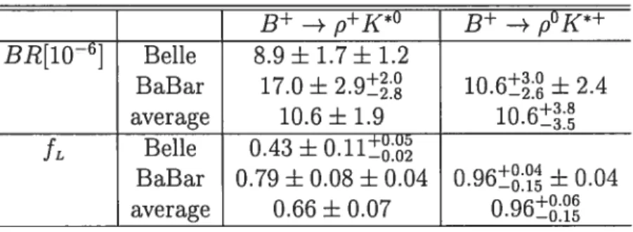
TAB. 4.1 — Branching ratios and polarization fractions for the two 3+ pK* decays. Data cornes from Ref.

_[381;

averages are taken frorn Ref. [39].

3+ p+K*D 3+ BR[l0—6] Belle 8.9 + 1.7 + 1.2 BaBar 17.0 ± 2.9j 10.6t + 2.4 a.verage 10.6+1.9 10.6t

h.

Belle 0.43 + 0.iij BaBar 0.79 + 0.08 + 0.04 0.96t + 0.04 average 0.66 + 0.07 0.96t

direct CP asymmetries and triple-prodllct asymmetries in both pK* modes would provide important constraints on the various amplitudes and their phases, thereby providing strong tests of the SM.

The above SM predictions can now be compared with the present B —+ pK

data, shown in Table 4.1. Using the central values, and using the SM relation A1 _Au, wefind E1 E1j 77%. This is very far from the expected value of zero, so that one might be tempted to daim the presence of new physics. However, even though the systernatic error /E1 /E11 is relatively small, r’J 20%, the statistical error is enormous, +129%. Thus, the errors are still much too large to daim any discrepancy with the $M. However, this does dernonstrate the importance of more precise measurements of the polarizations in B —+ pK decays.

Whule the predictions of Refs. [35,

361

are flot invalidated, the sarne is not truc for Ref. [37]. In this scenario, the fL fraction of both charged B — pK* decays is predicted to be greater than 90%. However, the data in Table 4.1 show that this clearly does not hold for 3 —+ p+K*, ruling out this SM explanation at the 3.5w

level.

Finally, we note that in the pQCD approach, even with annihilation and non factorizable effects, the large transverse polarization in B —* /K* cannot be ex

plained [40]. In Ref. [41], it is argued that one of the B —* K* form factors must

41 be doue, but the prediction of this scenario is then that the B —+ gK longitudinal polarization is smaller than that of both the B p+K* aid 3 pOI+* modes. The careful measurement of the polarization fractions in the B — pK* modes will test this scenario.

4.3 B —÷ nK Decays

There are four B —* 7cK decays. In the SM, neglecting srnall diagrams as usual,

their amplitudes are given by

A(B —* irK°) = p’

vA(3 — ir°Kj =

/4O+

= —T’e _— — _Pw,

A(3° —+ irK) = —T’e _— P,

—+ ir°K°) = P — P, , (4.16)

(Isospin implies the relation A°+/A° = A+•vA°°.) It is difficuit to explain

the present data (branching ratios, CP asymmetries) ilsing only this parametriza tion

_[11.

We therefore consider the addition of new —+ (q = u, cl) operators. One

can show that the strong phase of any NP operator is much smaller than that of the $M [22}. In this case, for a given type of transition, ail NP matrix elements can

now be combined into a single effective NP amplitude, with a single weak phase

(irK O B) qiq

(4.17)

in which the symbols  and ‘J denote the NP amplitudes and weak phases, respec tively. In B —÷ -irK decays, there are four classes of NP operators, differing in their

color structure Fjsc. and iFs Fjqc. (q = u, cl). The matrix elements

of these operators can be combined into single NP amplitudes, denoted

and !c,qi% respectively

_[421.

Each of these contributes differently to the variolls B —+ ‘irK decays. (Note that, despite the color-suppressed index C, the matrix

elemellts are lot necessarily smaller than the

ÂIei’..)

In the preserice of these NP matrix elements, the B —+ 1K amplitudes take the

form [1,421 + = —Pt — T’ e — +ÀI,c0mbe — A = —P — T’ — = — P,,, + Â’°’ + Alc,dez , (4.18)

where ,4!,combei’ _{—”e + A!,de.}

Even taking into account the fact that P and T’ are related jiZ], there are too many theoretical parameters to perform a fit. For this reason, the authors of Ref.

_[1

assumed that a single NP amplitude dominates. They considered four possibilities (i) only À!,comb

_#

o,

_{(ii) only Alcu 0, (iii) only Â’°” 0, (iv)}

=

A’e’, A’°’

= O (isospin-conserving NP). 0f these, only choice

(j) gave a good fit; the others produced poor or very poor fits’. The good fit found best-fit values of 4!comb/p! _{= 0.36 and T’/P’ = 0.22. Thus, the NF parameter}

was found to be larger than the tree amplitude, with Ac0mb/TI = 1.64.

In what follows, we assume that NP of type (i) is present in B —+ rrK decays. This same NP vi11 affect B —* pK* decays. In order to calculate the effect on the B —* pK polarization states, we must assume a particular form for A!,m) _There

are many NP operators which can contribute to A’°”. They are

{f

7As7Bq+gb7As77Bq}

. (4.19)

A,B=L,R

There are a total of 16 contributing operators (A, B = L, R, q = u, U); tensor

operators do not contribute to B —+ ii-K. For simplicity, we assume that a single operator contributes to A!,comb _{and we analyze their effects one by one.}

‘Note that the poor fit gave a discrepancy of only about 2g with the SM, so that, strictly speaking, it cannot be ruled out. However, in what follows, we concentrate on the good fit.